konz_thesis_draft_FINAL.pdf

(1)

Bayesian Model Fitting with Both Intrinsic and

Extrinsic Uncertainties in Two Dimensions

Nicholas Clayton Konz

Senior Honors Thesis

submitted to

Department of Physics and Astronomy

The University of North Carolina at Chapel Hill

Approved for Highest Honors:

Prof. Daniel Reichart, Thesis Advisor

Prof. Fabian Heitsch, Reader/Committee Member

Prof. Lu-Chang Qin, Reader/Committee Member

(2)

The LA_{TEX template from Karl Voit is based on} _{KOMA script}_{and can be found online:}

(3)

I declare that I have authored this thesis independently, that I have not used other than

the declared sources/resources, and that I have explicitly indicated all material which has

been quoted either literally or by content from the sources used.

Date Signature

(4)

Fitting a statistical model to data is one of the most important tools in any scientific

or data-driven field, and rigorously fitting a two dimensional model to data that has

intrinsic uncertainties (error bars) in both the independent variable and the dependent

variable is a daunting task, especially if the data also has extrinsic uncertainty (sample

variance) that cannot be fully accounted for by the error bars. Here, I introduce a novel

statistic (described as the Trotter, Reichart, Konz statistic, or TRK) developed in Trotter

(2011) that is advantageous towards model-fitting in this “worst-case data” scenario,

especially when compared to other methods. I implemented this statistic as a suite of

fitting algorithms in C++ that comes equipped with many capabilities, including: support

for any nonlinear model; probability distribution generation, correlation removal and

custom priors for model parameters; asymmetric uncertainties in the data and/or model,

and more. I also built an end-to-end website through which the algorithm can be used

easily, but generally, with a high degree of customizability. The statistic is applicable

to practically any data-driven field, and I show a few examples of its usage within

the realm of astronomy. This thesis along with Trotter (2011) form the foundations

for Trotter, Daniel E. Reichart, and Konz (2020), in preparation. The TRK source

code and web-based calculator can be found at https://github.com/nickk124/TRKand

(5)

Acknowledgements

To begin, I would like to acknowledge the support of the excellent Department of Physics

and Astronomy at UNC Chapel Hill, for its vibrant and closely-knit community of students

and faculty, its many excellent and brilliant professors, and the wonderful atmosphere of

learning and collaboration that is facilitated by everyone within. Without such a positive

and encouraging context, my research would have never become what it is today. Similarly,

I would also like to thank current and past members of the Reichart Lab/Skynet Robotic

Telescope Network for their support and collaboration throughout my time in the lab,

including Dylan Dutton, Vladimir Kouprianov, John Martin, and Roark Habeggar. I would

also like to specifically thank Prof. Fabian Heitsch, as both his course on physical modeling

and my consulting of his vast knowledge of numerical techniques and modeling for this work

equipped me to tackle a number of challenging problems. I would also like to acknowledge

the financial support of the NASA/North Carolina Space Grant Undergraduate Research

Fellowship and Scholarship Programs, as well as the UNC Department of Physics and

Astronomy in the form of the Earl Nelson Mitchell Scholarship in Physics, and the Robert

Shelton Award for Outstanding Research.

Without Adam Trotter, this thesis would not exist, and not just because his 2011 PhD

dissertation serves as the foundation for this work. Ever since I began work on this project,

Adam has been incredibly helpful and insightful. His attentiveness and rapid response

time toward my constant volley of questions is only matched by his immediate dedication

toward solving any problem I level at him. I very much look forward to continuing to

work with Adam in the future.

Dr. Daniel Reichart. Prof. Reichart, or Dan, is a man of many names and of many interests.

(6)

font of knowledge that he possesses, and his willingness to dive deep into any problem,

straight to the whiteboard, no matter how difficult it becomes. I have never met someone

with such rapid, full attentiveness and masterful way of elucidating difficult topics and

quickly figuring out (often unorthodox) solutions to new problems. Overall, Dan has not

just been indispensable to helping me with this project; he has been the driving motivator

for my entire research career over these past three years. Anybody would be extremely

(7)

List of Figures

2.1. Example dataset and underlying model distribution where the scatter of

the data cannot solely be accounted for by the error bars, which must be

parameterized as extrinsic scatter, orslop. Model distribution is shown with 1₋, 2₋ and 3σ confidence regions for the slop of the model, to properly

account for the uncertainty in the dataset. . . 5

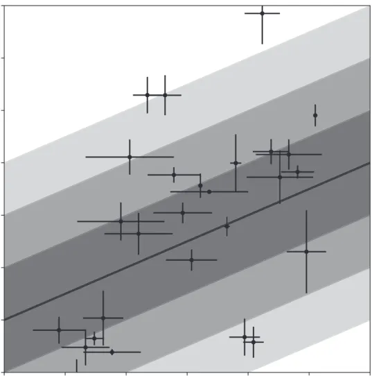
2.2. Visualization of some two-dimensional dataset (from Trotter (2011)) with

both intrinsic and extrinsic scatter in two dimensions, and accompanying

model distribution with 1₋, 2₋and 3σ confidence regions for the extrinsic

scatter/slop of the model represented by the shaded regions. Inset box is

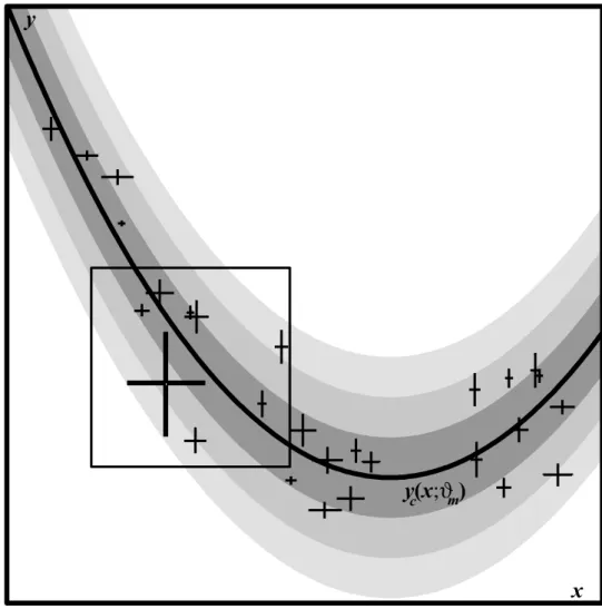
shown zoomed in Fig. 2.3. . . 7

2.3. Fig. 2.2, zoomed in, from Trotter (2011). Centered is a single

data-point (xn, yn) with intrinsic probability distribution defined by its’ error

bars/intrinsic scatterσx,n, σy,n, alongside a model distribution with curve yc(x;ϑm) and extrinsic scatter/slop parameters (σx, σy). The shaded re-gions represent the 1−, 2− and 3σ confidence regions of the datapoint’s

intrinsic probability distribution, and of the extrinsic scatter-convolved

model distribution. . . 8

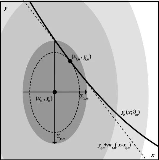
2.4. Visualization of some datapoint (xn, yn) with convolved error ellipse defined

by the extrinsic-intrinsic convolved error bars (Σx,n,Σy,n), alongside some

(10)

2.5. Illustration of the geometry of the TRK statistic modified from Trotter

(2011), given some datapoint and model. The datapoint is centered at

(xn, yn) (point O), with convolved error ellipse described by the widths (Σx,n,Σy,n) (Equation (2.9)). The model curve yc(x;ϑm) is tangent to the convolved error ellipse at tangent point (xt,n, yt,n) (pointT), and the red line is the linear approximation of the model curve, with slope mt,n = tanθt,n. The blue line indicates the rotated coordinate axisunfor the TRK statistic, perpendicular to the vn axis. . . 15 4.1. Example of a model curve yc(x;ϑm) (purple, top) and datapoint (xn, yn)

with convolved error ellipse (red, middle) described by (Σx,n,Σy,n) where there are multiple points where yc is tangent to the ellipse. This translates to there being multiple solutions/roots to/of Equation (2.13), which is

plotted in orange at the bottom. . . 24

4.2. Example of slop/extrinsic scatter (σx, σy) dependence on fitting scale s (for some linear model). Note that as is predicted in _§3.0.3, there exist

minimum and maximum scales s =a and s =b (respectively) such that lim

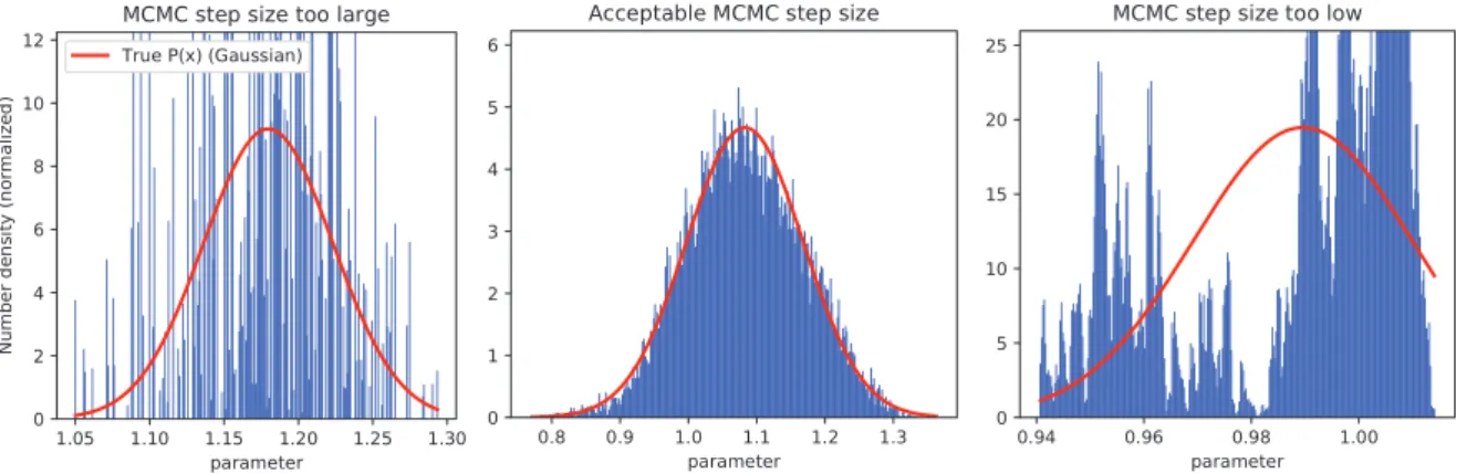
s→a+σx = 0 and lim_s_→_b−σy = 0. . . 30 4.3. Histograms of MCMC Metropolis-Hastings samplings for a normal-distributed

parameter m, with true Gaussian posterior plotted in red, given (Gaus-sian) proposal distribution widths/“step sizes” ofσm = 10, σm = 0.1, and σm = 0.0001, from left to right, given a sample size of R= 100,000. Note that even with such a high sample size, the choice of the step size for the

model parameter’s Markov Chain willdrastically change the quality of the sampling. . . 35

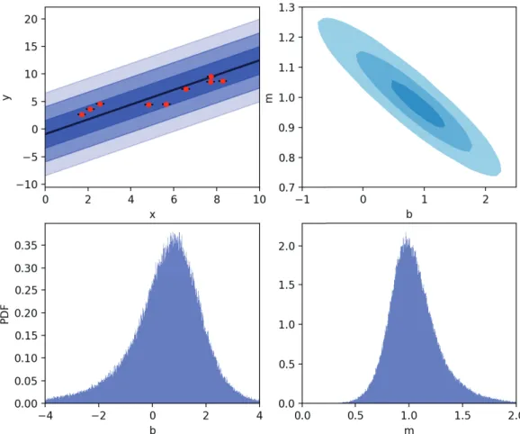
4.4. Top left: Example extrinsic scatter-dominated dataset (red) with small x−

andy₋ error bars (barely visible), alongside linear fit model distribution y = mx+b with 1−, 2− and 3σ slop confidence regions visible in blue. Top right: model parameter confidence ellipse with 1₋, 2₋ and 3σ regions

(11)

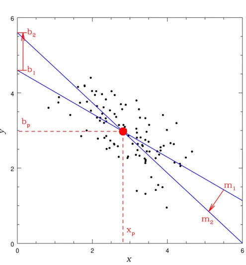
5.1. From Trotter (2011), this figure illustrates two different linear fits on the

same dataset, with both sets of model parameters b, m offset from some best fit b, m, representing the uncertainty in this best fit. As shown, both of these lines intersect at some optimum pivot point xp, plotted in red; if this optimal xp is chosen when fitting the model, the correlation between b and m will be minimized. . . 42 5.2. Ten different iterations for the MCMC-generated distributions of new

pivot pointsxnew

p computed with Equation (5.3) and weighted according to

Equation (5.7), overlapped. For each iteration we take the optimal value of

the new pivot point to be the weighted half-sample mode (see Bickel and

Fruehwirth (2005)) of that iteration’s distribution, and use this optimal

value asxold

p for the next iteration in order to compute the next distribution

of xnew

p . As can be seen (given that only four or so iterations are visible), I

have found this algorithm to converge quickly, usually only needing a few

iterations, if more than one is needed at all. . . 45

5.3. Top left: The same extrinsic scatter-dominated dataset as in Figure 4.4 but

now with pivot point xp in model y=m(x−xp) +b optimized to minimize correlation between b and m, using Algorithm 8. Model is shown with 1−, 2− and 3σ slop confidence regions visible in blue. Top right: model

parameter confidence ellipse with 1₋, 2₋and 3σ regions shaded, generated

from the posterior probability distributions for b and m found via MCMC, bottom. Note that with pivot point optimized, the confidence ellipse is now

no longer tilted as in Fig. 4.4, indicating the removal of correlation, also

(12)

5.4. From Trotter (2011), a visualization of the 2D joint probability for an

asymmetric model curve yc and data-point (xn, yn) with asymmetric error bars. This joint probability is an integral that can be approximated by

a 2D asymmetric Gaussian with widths (Σx,n±,Σy,n±) centered at some

(xn+δx,n, yn+δy,n). The integral is broken into three segments according to the quadrants about the convolved centroid (xn +δx,n, yn+δy,n), in this case I−+, I++ and I+−, respectively, with subscripts denoting which

quadrant the integral/linear approximation of the model curve is located

in. For this example, I−+ (red) through quadrant 2 has limits (−∞, x1],

I++ (green) through quadrant 1 has limits [x1, x2], and I+− (blue) through

quadrant 4 has limits [x2,∞). . . 50

6.1. From Trotter (2011), the combined CCM and FM extinction model curve

along a typical Milky Way line of sight. The y-axis is defined to be the ratio between the λ₋V color excess E(λ₋V) at a given wavelength λ, and the B₋V color excessE(B₋V), where the color excess is defined as the difference, in magnitudes, of the absorption due to dust at two given

wavelengths. In this case,B andV correspond to wavelengths in the middle of standard blue and visible photometric filters. The color excess ratio

plotted on the y-axis is thus proportional (with an offset) to the magnitude of dust extinction at a given wavelength λ. The x-axis is proportional to the inverse of λ, specifically x_≡(λ/1 µm)−1_{, or, equivalently, proportional}

to frequency. As shown, the parametersc1 andc2 describe the intercept and

slope of a linear component of the model. The parameter γ parameterizes the width of the “bump” in the center of the model (also known as the

“UV bump”), while the parameter BH≡c3/γ2 describes the height of this

bump. . . 60

6.2. Observed c1 vsc2 data from Valencic, Clayton, and Gordon (2004), Gordon

et al. (2003), E. Fitzpatrick and Massa (2007), and Clayton et al. (2015),

plotted with linear TRK fit modeled by Equation (6.4). Shaded regions

indicate the 1₋, 2₋and 3σslop confidence regions of the model distribution,

given best fit slop values of Table 6.2.1 and plotted according to footnote

(13)

6.3. MCMC-generated (_§4.4.1) probability distributions for c1 vs. c2 (Equation

(6.4)) model (top) and slop/extrinsic scatter (bottom) parameters.

Param-eter confidence ellipses (center) with 1₋, 2₋ and 3σ regions show joint

posterior probabilities with respect to the parameters plotted on either side.

The pivot-point finding algorithm of_§5.1 was used to remove correlation

between model parameters.. . . 63

6.4. Observed BH vsc2 data from Valencic, Clayton, and Gordon (2004), Gordon

et al. (2003), E. Fitzpatrick and Massa (2007), and Clayton et al. (2015),

plotted with broken-linear TRK fit modeled by Equation (6.5). Shaded

regions indicate the 1₋, 2₋ and 3σ slop confidence regions of the model

distribution, given best fit slop values of Table 6.2.2 and plotted according

to footnote 19 on page 39. . . 66

6.5. MCMC-generated (§4.4.1) probability distributions for BH vs.c2 (Equation

(6.5)) model (top and middle rows) and slop/extrinsic scatter (bottom row)

parameters. Parameter confidence ellipses (center) with 1−, 2− and 3σ

regions show joint posterior probabilities with respect to the parameters

plotted on either side. The pivot-point finding algorithm of §5.1 was used

to remove respective correlations between model parameters of each linear

”leg” of the model curve. . . 67

6.6. The data input step of the web-based TRK calculator with example data. 68

6.7. Example of plotting input data on the TRK calculator webpage. . . 69

6.8. Section of the TRK webpage where the user can choose which model to fit

to their data. . . 70

6.9. Section of the TRK webpage where the user can determine which additional

TRK algorithms to run alongside basic fit. . . 71

6.10. Output section of the TRK calculator webpage, showing the results of an

(14)

Robustly fitting a statistical model to data is a task ubiquitous to practically all

data-driven fields, but the more nonlinear, uncertain and/or scattered the dataset is, the

more difficult this task becomes. In the common case of two dimensional models (i.e.

one independent variable x and one dependent variable y(x)), datasets with intrinsic

uncertainties, or error bars, along both xand y prove difficult to fit to in general, and if

the dataset has some extrinsic uncertainty/scatter (i.e., sample variance) that cannot be

accounted for solely by the error bars, the difficulty increases still.

In this work, I describe a new, easily generalizable statistic developed by Trotter (2011),

the Trotter-Reichart-Konz statistic—hereafter the TRK statistic—that is used to fit

models to data in such “worst case” scenarios. Such model distributions are defined by

convolving a model curve yc(x;ϑm) that describes the shape of the model with a 2D

probability distribution that characterizes the scatter of the data, where ϑm is the set of

parameters describing the model. In order to fit such a model to a set of data, values

for ϑm and the parameters that describe the extrinsic scatter of the dataset must be

determined that maximize the joint probability, or likelihood, of the model curve and

the dataset; in other words, a model distribution must be found that is most likely to

reproduce the dataset. Assuming that the intrinsic and extrinsic uncertainties are Gaussian

(possibly asymmetric), I show how to define such a likelihood function following Trotter

(2011). This likelihood includes integrating over a rotated coordinate system of choice,

and when a specific set of coordinates is used, it results in a statistic that is invertible (i.e.

fitting x vs. y will result in the same fit asy vs x), computationally feasible, and reduces

to a χ2 _{statistic in the classic 1D uncertainty case; we define this as the TRK statistic.}

Models predicted by maximizing the TRK statistic’s likelihood function are geometrically

(15)

datapoint centroid from the model curve, which I demonstrate. As such, the statistic is

χ2_{-like, measured in the direction of closest approach of the model curve to the datapoint.}

The TRK statistic is not scalable, i.e. it yields different best fits depending on the choice of

basis, orscale for each coordinate axis, with some optimum scale corresponding to the true

best fit. However, I present an implementation of an algorithm originally conceptualized

in Trotter (2011) that can determine such an optimum scale, effectively removing this

caveat of the TRK statistic.

The original introduction of the TRK statistic in Trotter (2011) used a genetic

algorithm-based implementation of the statistic that was non-automated, non-“production style”

code that only demonstrated the proof-of-concept of the statistic, rather than introduced

an easy-to-use, widely applicable codebase. Because of this, my contribution to TRK

was to implement the statistic from scratch into a fully-fledged, general nonlinear fitting

suite that can be picked up and used easily by anyone, while supporting a number of

features. This codebase is the focus of this work, and can be found, with documentation,

athttps://skynet.unc.edu/rcr/calculator/downloads.

In §2 and §3 I introduce the TRK statistic and its central properties, closely following

Trotter (2011). Following this, in _§4 I introduce the core algorithms used to perform fits

and other procedures with the TRK statistic in practice, including, but not limited to, fit

scale optimization, determining best fits, and model parameter distribution generation.

Then, in §5 I introduce additional algorithms of the TRK suite, including methods for

the removal of correlation between model parameters, and the addition of asymmetric

extrinsic and/or intrinsic uncertainties.

In _§6I begin by comparing the TRK suite to similar algorithms (_§6.1), and then present

TRK fits used to model relationships between empirical parameters that describe the

extinction of light by dust in the Milky Way as examples of the usage of the suite

(§6.2). Next, I present a robust but easy-to-use implementation of the algorithm into a

webpage-based calculator that I developed end-to-end (_§6.3), which can be used for quick,

reliable fitting while also possessing a number of features. Finally, in §7I discuss potential

(16)

2.1. Statistical Preliminaries: Bayesian Statistics

I begin by considering some set of observed data D and a set of parameters H that

describes some hypothetical model for this data. From here, I define p(H) to be the prior

probability distribution function, or prior for short; this defines how any prior information

known about the model parameters (before data collection) affects and/or constrains

the value of such parameters. For example, if some parameter has a best fit value and

uncertainty from a previous result, this can form the basis of a prior for that parameter.

Next, we define the likelihood probability distribution function L(D|H), or likelihood for

short, as the conditional probability of obtaining the observed dataD given some model

described by H; this is the term that describes how likely the model is to have generated

the data. Finally, in order to examine how some model described byH can arise from the

data, we define the posterior probability distribution functionp(H|D), or posterior for

short, to be the probability of obtaining certain model parameters H given the data D.

These quantities can all be related with Bayes’ Theorem

p(H|D) = L(D|H)p(H)

p(D) , (2.1)

of which the proof is outside the scope of this work, but is found in any introductory

probability course. In Equation (2.1) the normalization factorp(D), known as theevidence,

is typically difficult to compute. However, really only being a normalization factor, it can

(17)

in this work, Bayes’ Theorem will be used in the form of

p(H|D)∝ L(D|H)p(H). (2.2)

From here, its clear that given some prior(s) p(H), if a likelihood function _L(D_|H) can be

defined, then the posterior can be determined, which ultimately describes the distribution

of the model parameters that arise from the dataset. The central goal of the remainder of

this chapter will be to clearly define this likelihood.

2.2. Fitting a Model to Data in Two Dimensions

Consider a set of N two-dimensional datapoints {xn, yn}, where n = 1,2, . . . N. In the

most general case, each datapoint has an intrinsic probability distribution defined by its

intrinsic scatter/statistical uncertainty, orerror bars for short,{σx,n, σy,n} along one or

both dimensions of x andy1_{. The dataset can also have} _{extrinsic scatter}_/_{sample variance}_,

or slop for short, again in both dimensions, that cannot solely be accounted for by the

error bars (see Fig. 2.1 for an example). In this case, the slop must be parameterized and

fit to as part of the model. Hereafter, unless otherwise stated, I assume that the slop

is normally distributed along the two dimensions and described by the two parameters

σx and σy, that are constant along the entire dataset. I also assume that the intrinsic

scatter in both dimensions, and the extrinsic scatter in both dimensions, are respectively

uncorrelated.

In the following section, we will begin to explore how a likelihood function describing a

model for this “worst case” type of dataset can be defined, by connecting the extrinsic

and intrinsic probability distributions of the dataset with the model itself.

1_{The data can also be given weights}

{wn}, i.e. assigning some datapoint a weight of 2 is equivalent to

(18)

(19)

2.2.1. The Likelihood Function

The derivation below closely follows Trotter (2011), where the TRK statistic was initially

formulated. In order to consider fitting a model to data, we must first determine how to

quantify the goodness of fit for such a model, given some distribution ofN measurements

described in the previous section. I define part of the model as some probability distribution

g(x, y) that is convolved along some model curve function yc(x;ϑm), where ϑm is the set

of parameters that define the functional form of the model; here, g(x, y) can be thought of

as the ”density function” of the model distribution. Then, in order to properly represent

the scatter of the data, I define the full model distribution by convolving this with a 2D

Gaussian distribution that characterizes the slop, with widths defined by the parameters

σx and σy. This representation of the model can be difficult to conceptualize, but it is

necessary in order to work with the most general, Bayesian treatment of a two-dimensional

uncertain dataset. A visualization of this is shown in Figures2.2 and 2.3.

Another way to express the (effectively 1D) model curve yc(x;ϑm) is do describe it as

a one-dimensional delta function along some arbitrary chosen (orthogonal) coordinate

system (un, vn). Indicated by the subscripts ofn, such coordinates can, in the most general

case, vary between datapoints. As such, we can express the probability density along the

model curve as g(x, y)δ(vn, vc,n(un;ϑm)), where vc,n(un;ϑm) is yc(x;ϑm) in the (un, vn)

coordinate system, and δdenotes the one-dimensional Dirac delta function. Also note that

given that the coordinates (un, vn) are assumed to be orthogonal, we can always express

them as a rotation from (x, y).

Now that we have an expression for the probability density along the model curve, we

can convolve this with the extrinsic scatter/slop distribution (again, assumed to be 2D

Gaussian) to obtain the model distribution function for a single datapoint,

pmod

n (x

0

, y0|ϑm, σx, σy) =

Z

un Z

vn

g(x, y)δ(vn, vc,n(un;ϑm))N(x0|x, σx)N(y0|y, σy) dvndun,

(2.3)

(20)

y

_c

(

x

;ϑ

_m

)

x

y

(21)

x

y

_c

(

((

x

;ϑ

)

y

((

;ϑ

_m

σ

_x,n

σ

_y,n

σ

(

x , y

y

((

_{n n}

, y

)))

σ

_y

σ

_x

σ

Figure 2.3.: Fig. 2.2, zoomed in, from Trotter (2011). Centered is a single data-point (xn, yn) with intrinsic

probability distribution defined by its’ error bars/intrinsic scatterσx,n, σy,n, alongside a model

distribution with curveyc(x;ϑm) and extrinsic scatter/slop parameters (σx, σy). The shaded

(22)

both over (_−∞,_∞) and_N denotes the Gaussian/normal distribution

N(x0|µ, σ) = √ 1

2πσ2exp

−1

2

(x0 ₋_µ₎2

σ2

. (2.4)

with mean µ and standard deviation σ.

Next, we need to obtain an expression for the full joint probability of a single datapoint

with the model distribution function pmod

n for that datapoint. The intrinsic probability

for a single datapoint comes from the error bars for that datapoint, and is found with

pint

n (x

0_{, y}0

|xn, yn, σx,n, σy,n) =N(x0|xn, σx,n)N(y0|yn, σy,n). (2.5)

again assuming Gaussian error bars. From here, we can find the joint probability of

some nth _{datapoint with the model distribution by integrating the product of the two}

distributions pmod

n and pintn over x0 and y0, as

pn(ϑm, σx, σy|xn, yn, σx,n, σy,n) =

Z

x0

Z

y0

Z

un Z

vn

g(x, y)δ(vn−vc,n(un;ϑm))×

N(x0|x, σx)N(y0|y, σy)N(x0|xn, σx,n)N(y0|yn, σy,n) dvndundy0dx0. (2.6)

Next, the likelihood function is defined to be the product of allN of the joint probabilities

of the datapoints, as

L=

N

Y

n=1

pn(ϑm, σx, σy|xn, yn, σx,n, σy,n), (2.7)

so in theory, our work of finding an expression for the likelihood is done. However, given

the four integrals in Equation (2.6), this solution is quite computationally intractable. In

order to obtain a practical likelihood, a few simplifying, but reasonable approximations

(23)

2.2.2. An Analytical Approximation of the Likelihood

To begin, we can simplify the expression for the joint probability pn by noting that the

(x0_{, y}0_{) integral in Equation (2.6) can be evaluated analytically, which gives}

pn(ϑm, σx, σy|xn, yn, σx,n, σy,n) =

Z

un Z

vn

g(x, y)δ(vn−vc,n(un;ϑm))N(x|xn,Σx,n)N(y|yn,Σy,n) dvndun, (2.8)

where (Σx,n,Σy,n) are the quadrature sums of both the intrinsic and extrinsic scatters:

Σx,n ≡ σx,n2 +σ

2

x

1/2

Σy,n ≡ σy,n2 +σ

2

y

1/2

. (2.9)

What is the significance of these terms? In the words of Trotter (2011), Equation (2.8)

indicates that the joint probability of some nth _{datapoint with the model distribution is}

proportional to the integral of the effectively one-dimensional probability density along

the model curve through a two dimensional convolved Gaussian, whose widths are the

quadrature sums of the intrinsic and extrinsic uncertainties in each direction, Σx,n and

Σy,n. In other words, Fig.2.3 is equivalent to2.4.

To further simplify Equation (2.8) (i.e., remove the integrals), I’ll begin by making the

first approximation: that the intrinsic probability density along the model curve g(x, y)

varies slowly with respect to the scale of the size of the convolved error ellipse described by

Σx,n and Σy,n. This will makeg(x, y) approximately constant, such that it can be pulled

out of the integral in Equation (2.8). Next, I will assume that the model curve yc(x;ϑm)

is approximately linear over this same scale; specifically, I will approximate yc as a line

yt,n(x) passing through the point (xt,n, yt,n) where yc is tangent to the convolved error

ellipse, with some slope mt,n (see Fig. 2.4), i.e.

yc(x)≈yt,n+mt,n(x−xt,n). (2.10)

(24)

Σ

x,n

Σ

y,n

(

x

_{n n}

,

y

)

(

x

,

y

)

t,n t,n

y

x

y

+

m

(

x-x

)

t,n t,n t,n

y

(

x

;

J

)

c m

Figure 2.4.: Visualization of some datapoint (xn, yn) with convolved error ellipse defined by the

extrinsic-intrinsic convolved error bars (Σx,n,Σy,n), alongside some model curve yc(x). Also shown

(25)

(xt,n, yt,n), then we have the relation

(yc(x;ϑm)−yn)2

Σ2

y,n

+(x−xn) 2

Σ2

x,n

= (yt,n−yn) 2

Σ2

y,n

+ (xt,n−xn) 2

Σ2

x,n

, (2.11)

which is the condition for (x, yc(x;ϑm)) to be a tangent point. Differentiating this equation

with respect to x gives

d dx

(yc(x;ϑm)−yn)2

Σ2

y,n

+ (x−xn) 2

Σ2

x,n

= 0, (2.12)

which implies that the tangent point is equivalent to the point on yc that minimizes the

radial distance to the centroid of the error ellipse. Evaluating the derivative gives us an

equation that can be implicitly solved for x=xt,n,

(yc(x)−yn)

dyc(x;ϑm)

dx Σ

2

x,n+ (x−xn)Σ2y,n= 0, (2.13)

given some model curve and datapoint.

Finally, given these two assumptions, the joint probability of the nth _{datapoint and the}

model distribution of Equation (2.8) can be simplified by integrating over vn, as

pn(ϑm, σx, σy|xn, yn, σx,n, σy,n)≈g(xn, yn)

Z ∞

−∞N

(x|xn,Σx,n)N(yc(x;ϑm)|yn,Σy,n) dun,

(2.14)

given the “selecting” property of the delta function on the Gaussian along y. By using

the chain rule substitution dun= d_du_xn dx, yc(x;ϑm)≈yt,n+mt,n(x−xt,n) from Equation

(2.10), and integrating over x, we have finally arrived at an analytic expression for pn:2

pn(ϑm, σx, σy|xn, yn, σx,n, σy,n) (2.15)

≈g(xn, yn)

dun

dx N

yn|yt,n+mt,n(xn−xt,n),

q

m2

t,nΣ2x,n+ Σ2y,n

.

The likelihood function is the joint probability of the model distribution with all of the

2_{Here, we have also implicitly made an additional approximation: that the efficiency of which the}

measured data samples the true model distribution is approximately constant along the scale(s) of (σx,n, σy,n) and (σx, σy). This is unnecessary to delve into for the purposes of this work, but for an explicit

(26)

datapoints, and the best fit model parameters are defined as the parameters that, when

plugged into the likelihood, maximize it. In other words, the likelihood is the product of

all N of the individual datapoints’ joint probability distributions. In practice, rather than

choosing to maximize _L to determine the best fit, it is much more common to minimize

−2 ln_L (or some proportion thereof) in order to determine the best fit model parameters, for reasons of computational flexibility. In the simplifying “traditional” case of no error

bars inxand no slop whatsoever,−2 lnLis equivalent to theχ2 _{“goodness-of-fit” statistic,}

χ2 ₌ PN

n=1

[(y₋yc(x;ϑm))/σy,n]

2

. As such, in our general case, ₋2 ln_L is analogous to χ2_,

and has the form of

−2 lnL=−2

N

X

n=1

lnpn(ϑm, σx, σy|xn, yn, σx,n, σy,n)

=

N

X

n=1

[yn−yt,n−mt,n(xn−xt,n)]

2

m2

t,nΣ2x,n+ Σ2y,n

−2 N X n=1 ln  

dun

dx

1

q

m2

t,nΣ2x,n+ Σ2y,n



+C ,

(2.16)

following Equations (2.7) and (2.15), where C is a constant3_.

Recall that the rotated coordinate system (un, vn) in which the 1D model curveδ(vn, vc,n(un;ϑm))

is defined can be chosen at will, including the usage of different coordinates for different

datapoints. As will be described in _§6.1, different choices of these coordinates/of dun

dx will

give different statistics, with noticeably different properties. The following section will

show how a certain choice of these coordinates will lead to the TRK statistic.

2.2.3. The TRK Likelihood

As shown in Equation (2.16), The arbitrary choice of the rotated coordinates (un, vn) and

therefore the factor dun

dx will be what defines a given statistic. While various choices for

dun

dx that lead to different statistics with different properties will be explored in §6.1, for

now I will only examine the choice that leads to the TRK statistic, which is advantageous

over other such statistics for reasons that will be addressed in §6.1.

3_{The explicit form of the constant}_C _{is given in Trotter (}₂₀₁₁_{), which isn’t necessary for the purposes}

(27)

The TRK statistic is defined such that for some nth _datapoint, _u

n is chosen to be

perpendicular to the line segment connecting the centroid of the datapoint (xn, yn) with

the tangent point (xt,n, yt,n) discussed in the previous section. This choice results in a

likelihood of the form

LTRK

∝

N

Y

n=1

s

m2

t,nΣ2x,n+ Σ2y,n

m2

t,nΣ4x,n+ Σ4y,n

exp

(

−1₂[yn−yt,n−mt,n(xn−xt,n)]

2

m2

t,nΣ2x,n+ Σ2y,n

)

−2 lnLTRK =

N

X

n=1

[yn−yt,n−mt,n(xn−xt,n)]2

m2

t,nΣ2x,n+ Σ2y,n

−

N

X

n=1 ln

_m2

t,nΣ2x,n+ Σ2y,n

m2

t,nΣ4x,n+ Σ4y,n

+C ,

(2.17)

which is the central equation of this work. One important property of the TRK statistic is

thatit is essentially a one-dimensional χ2_{-like statistic that is measured in the direction of}

the tangent point4_{. For a visualization of the geometry of the TRK statistic, see Figure}_2.5.

Hereafter, I will sometimes use the shorthand χ2

TRK ≡ −2 lnLTRK, especially in Chapter 4 where it is frequently used.

(28)

x

m Σ_t,n

Σ_x,n

Σ y,n

y _cx- y

Yn

O

T

u_n

θ t,n

Figure 2.5.: Illustration of the geometry of the TRK statistic modified from Trotter (2011), given some datapoint and model. The datapoint is centered at (xn, yn) (pointO), with convolved error

ellipse described by the widths (Σx,n,Σy,n) (Equation (2.9)). The model curveyc(x;ϑm) is

tangent to the convolved error ellipse at tangent point (xt,n, yt,n) (pointT), and the red line

is the linear approximation of the model curve, with slope mt,n = tanθt,n. The blue line

(29)

3. Properties of the TRK Statistic

3.0.1. Invertibility

A useful property for any two-dimensional statistic is that it is invertible, i.e. that if fitting

a dataset’s y vs x data gives some model curve yc(x), fitting x vs. y gives the inverse

xc(y) =yc(x)−1. In the Bayesian formalism, a statistic is invertible if running these two

inverted fits yields the same likelihood function (Trotter (2011)). While mainly known to be

used as a measure of the linear correlation of a dataset, one metric of invertibility is actually

the ubiquitously-used Pearson Correlation Coefficient, R2_{, of Pearson (1896). To see this,}

consider some linear model with slope myx that was obtained by fitting to some y vs. x

data. Similarly, fitting x vs. y for the same dataset gives some model line with slopemxy.

As shown in Trotter (2011), the correlation coefficient can then be found as R2 _≡_m

xymyx;

therefore, if the statistic used to fit is invertible, and therefore mxy = 1/myx, we have

that R2 _{= 1. Proved by Trotter (2011),} _{the TRK statistic is completely invertible}_.

Therefore, by definition R2 _{= 1 always for the TRK statistic, meaning that fitting results}

can always be trusted under inversion.

3.0.2. Scalability

Another important property of any statistic, although not immediately obvious, is its

scalability. Here, a statistic is defined to be scalable if re-scaling the data along the x₋

or y− axis does not change the best fit arrived at from maximizing the likelihood. If a

statistic is not scalable, then the best fit willdepend on the choice of units of measurement,

which can easily create unwanted behavior when fitting (see e.g. Trotter (2011)), given

(30)

To examine the scalability of the TRK statistic, we will begin by noting that the statistic

is invariant if both x₋ and y₋ axes are rescaled by the same factor, shown in Trotter

(2011). As such, any rescaling that potentially affects the TRK statistic can always be

defined as rescaling only they₋axis by some numerical factor s1_{. In order to see the effect}

of data rescaling within the TRK statistic, I multiply ally₋axis dependent terms by some

s within the TRK likelihood of Equation (2.17), which gives

LTRK

s ∝ N

Y

n=1

s

m2

t,nΣ2x,n+ Σ2y,n

m2

t,nΣ4x,n+s2Σ4y,n

exp

(

−1

2

[yn−yt,n−mt,n(xn−xt,n)]2

m2

t,nΣ2x,n+ Σ2y,n

)

6∝ LTRK

for a fixed s . (3.1)

As such, the standalone TRK statisic is not scalable, so different choices of scale will

result in different best fit model parameters, including slop/extrinsic scatter (σx, σy). Not

only this, but it is impossible to determine anything about the relative fitness of best fits

solely given numerical values of the likelihood function; what this means in practice is

that the scaling factors can not be fit to as a model parameter (Trotter (2011)). However,

we will show in the following section that there is a way to quantitatively compare TRK

fits done at different scales, so that this hurdle can be negated.

3.0.3. The TRK Correlation Coefficient

To begin, consider two TRK best fits gained from maximizing the likelihood (Equation

(3.1)) at different scales (i.e. different values for s), given some model and dataset. Because

the TRK statistic is completely invertible, the Pearson Correlation Coefficient R2 _{is 1 for}

both fits. As such, in order to compare the two fits, a new correlation coefficient needs

to be defined that can quantify the variance of the statistic’s predictions between them.

By convention, the new coefficient should follow similar properties to R2_{, insofar that}

it is restricted to the range of [0,1], and that it equals 1 if the two best fit lines being

compared have the same slope (plotted in the same scale space).

I will begin with the case of linear fits, and continue on to generalize to arbitrary non-linear

1_{Equivalently we can define}_s

≡sy/sx, wheresy is the standalone rescaling of they−axis, andsx is

(31)

models. Trotter (2011) introduced a new correlation coefficientR2

TRK that is a function of thedifference of the slopes of the models, rather than theratio, as opposed to the Pearson

R2 _(see _§_{3.0.1). The}_{scale-dependent} _{TRK correlation coefficient is defined as}

R2

TRK(a, b)≡tan2

π

4 −

|θa−θb|

2

. (3.2)

given a linear fit at s = a with slope ma = tanθa, and another at s = b with slope

mb = tanθb2.Note that these fits, although performed at different scales, have their angles

compared within the original, s= 1 space. Clearly, if the two lines have the same slopes,

R2

TRK = 1 as desired, and if the two lines differ in slope angle by 90◦, i.e. they are orthogonal, R2

TRK = 0. Now that the difference between TRK fits at different scales can be compared, how do we determine the best scale at which to run a fit?

Consider how rescaling will affect the slop parametersσx and σy, i.e. how the total slop

is distributed between these two parameters. Trotter (2011) showed that in the limit of

slop-dominated data (i.e. arbitrarily small/zero error bars {σx,n, σy,n} as compared to

the extrinsic scatter/slop), s _→0, σx → 0; similarly, as s→ ∞, σy →0. This behavior

occurs because as the scale s of the dataset is changed, the distribution of the total slop

between σx and σy is correspondingly affected. This range of s ∈ [0,∞) is considered

to be the physically meaningful range of fits. In the case of a dataset with non-zero

error bars, this physically meaningful range becomes some subset interval [a, b]_⊂[0,_∞),

where the number a is described as the minimum scale, while b is the maximum scale,

as lim

s→a+σx = 0 and lim_s_→_b−σy = 0 (from Trotter, 2011)

3_{. As any fits done outside of this}

interval are inherently unphysical, there must be some optimum s0 ∈[a, b] that is the best

scale at which to run a fit4_.

In order to determine the optimum scale s0, the following iterative approach defined

within Trotter (2011) is used. To begin, the first approximation ofs0,s(1)₀ , is found to be

the scale at which

R2

TRK(a, s (1) 0 ) =R

2 TRK(s

(1)

0 , b)≡R 2

TRK. (3.3)

2_R2

TRK compares theangles (off of thex-axis) (θa, θb) of the lines rather than theslopes (ma, mb) for

numerical efficacy, given that the former are restricted to the range of ₋π₂,π₂, while the latter can be anywhere within (_−∞,_∞).

3_{Here, I’ve taken the signs of the limits to indicate the direction of one-sided approach.} 4_{By “unphysical”, I mean that such scales require imaginary best fit slops, i.e. (}_σ2

x, σ2y)<0 (Trotter,

(32)

From here, we shift from thes = 1 space to thiss =s(1)0 space, where the angles of the

lines follow the transformation θ _→arctans(1)₀ tanθ. The analysis of Equation (3.3) is

then repeated in this new space to determine the next approximation for the optimum

scale, s(2)₀ , i.e. finding the s(2)₀ such that, e.g. in the case of a linear model,

R2

TRK ≡tan 2   π 4 − arctan

s(1)0 tanθa

−arctans(1)0 tanθ_s(2) 0 2  

= tan2

  π 4 − arctan

s(1)0 tanθ_s(2) 0

−arctans(1)0 tanθb

2



 , (3.4)

where θ_s(2)

0 is the position angle of the best-fit line at scales

(2)

0 , as measured in s= 1 space. From here, we set s(2)₀ _→s(1)₀ , and repeat until convergence to the final value of s0. It is at

this optimum scale that we actually run fits, compute model parameter uncertainties (see

§4.4.1), etc. The details of how Equation (3.3) is solved in practice to determine s0 are given in §4.3.

The TRK correlation coefficient as given in Equation (3.2) can only be used for linear

models. As such, Trotter (2011) presented a logical generalization to nonlinear models, as

the average of the differences of the slope angles at allN tangent points at two scales a

and b:

R2

TRK(a, b)≡ 1 N N X n=1 tan2 π 4 −

|θt,n;a−θt,n;b|

2

. (3.5)

Here, θt,n;a= arctanmt,n;a and θt,n;b = arctanmt,n;b are the position angles of the best-fit

curves at the tangent point to the nth _{datapoint at scales} _a _and _b_{, respectively. This}

expression forR2

TRK can then be used to determine s0 using the same method described by the previous section and Equation (3.3); in this case then, Equation (3.4) becomes

R2 TRK ≡ 1 N N X n=1 tan2   π 4 − arctan

s(1)₀ tanθt,n;a

−arctans(1)₀ tanθ_s(2) 0 2   = 1 N N X n=1 tan2   π 4 − arctan

s(1)₀ tanθ_s(2) 0

−arctans(1)₀ tanθt,n;b

2



. (3.6)

(33)

are needed to describe how TRK fits are completed in practice. In the next chapter, I

will delve into the suite of algorithms that I created to perform fitting, scale optimization,

(34)

Algorithms

The previous chapter introduced all of the formalism needed to use the TRK statistic

in principle, but how can TRK fits be done in practice? What are the implementational

details? What options and configurations are available when using the TRK statistic?

While the statistic itself was created by Trotter (2011), it was only implemented in the form

of a genetic algorithm-based scientific codebase for testing. In order to have a

production-quality codebase for the usage of TRK, I created a new suite of algorithms from scratch in

C++, that completely overhauls how TRK fits are computed, including many additions and

optimizations as compared to the previous codebase. With this new codebase, TRK can

be used in a fully customizable, yet easy-to-use manner, with a host of options. The code

and full documentation can be downloaded athttps://github.com/nickk124/TRK.

The first part of this chapter will discuss the implementation of the central part of the

TRK statistic, the TRK likelihood function LTRK _{of Equation (2.17), that is maximized}

to obtain best fits. Here, I will explore my the algorithms that I use to determine the

tangent points described by Equation (2.13), and maximize LTRK _{with respect to all}

model parameters—including slop—to obtain best fits. Following this, I will delve into

the routine that is used to determine the optimum fitting scale s0, using the formalism

described in _§3.0.3. From there, I will explore the Monte Carlo methods used to generate

(35)

4.1. Tangent Point Finding

As shown in _§2.2.2 and_§2.2.3, for a given model curveyc(x;ϑm) and datapoint (xn, yn),

the point where the convolved error ellipse of the datapoint described by the convolved

error parameters (Σx,n,Σy,n) of Equation (2.9) is tangent to the model curve, (xt,n, yt,n), is

a central part of the TRK likelihoodLTRK _{(Equation (2.17)). Any time that the likelihood}

must be computed for a new set of model and slop parameters, all N of these tangent

points must be re-computed, and efficiently.

Recall that in order to determine such a tangent point xt,n (and therefore yt,n =

yc(xt,n;ϑm)), Equation (2.13) must be solved implicitly forxt,n in the general case of some

nonlinear model. In more practical terms, this means that the root(s) along the x₋axis

of the left hand side of Equation (2.13) are such tangent point(s). To determine these

tangent points, I use (a slightly modified version of) the Two-Point Newton-Raphson

algorithm created by Tiruneh, Ndlela, and Nkambule (2013) to find the roots of Equation

(2.13). This algorithm has a number of benefits over other root-finding methods such

as bisection and the traditional Newton-Raphson method, especially when dealing with

complicated nonlinear functions that otherwise give convergence and speed issues. My

pseudocode implementation of it is shown in Algorithm1.

It is essential to note that for certain non-monotonic, nonlinear models, there can easily be

multiple tangent points for a given datapoint; see Figure 4.1as an example. In this case, I

take the tangent point that maximizes the joint posterior probability1 _{as the tangent point}

to be used when evaluating the likelihood. However, only using the rootfinder of Algorithm

1 once per datapoint is insufficient, as some initial guess for the algorithm will always

only return the same, single tangent point. In order to reliably determine all possible

tangent points for a given datapoint, to properly maximize the likelihood, I use a logical

routine described in Algorithm 2. The goal of this routine is to determine various initial

guesses to supply to the root-finder until all possible tangent point-finding options have

been exhausted. To begin this algorithm, the root finder is used with the default initial

guess to determine the first tangent point. From here, I use a quadratic approximation (of

Equation (2.13)) through this first tangent point to approximate up to two more tangent

1_{I.e. for some}_nth_{datapoint, the joint posterior probability is the}_nth _{term in the product of Equation}

(36)

Algorithm 1: Modified Two-Point Newton-Raphson algorithm for finding a single tangent point.

1 Function TwoPointNR

Input :Model parametersϑm, datapoint (xn, yn), its convolved errors

(Σx,n,Σy,n), and initial tangent point guess of xguess.

Output :xt,n

2 begin

3 Initialize guess ofx_k−1 =xguess and xk=xguess+ Σx,n/

√

10)

4 while not converged do

5 Main Two-Pt NR loop:

6 y_k−1 = [yc(xk−1;ϑm)−yn]

dyc(xk−1;ϑm)

dx Σ

2

x,n+ (xk−1−xn)Σ2y,n

7 y_k = [y_c(x_k;ϑ_m)−y_n]dyc(xk;ϑm)

dx Σ

2

x,n+ (xk−xn)Σ2y,n

8 dyk

dx =

dyc(xk;ϑm)

dx

2

+ [yc(xk;ϑm)−yn]

d2_y

c(xk;ϑm)

dx2 Σ 2

x,n+ Σ

2

y,n

9 r= 1− yk

yk−1

yk−yk−1

xk−xk−1

dyk

dx

10 x_k₊₁ =

1₋ 1

r

xk−1 +

xk

r

11 x_k−1 =xk, xk=xk+1

12 end

(37)

Figure 4.1.: Example of a model curve yc(x;ϑm) (purple, top) and datapoint (xn, yn) with convolved

error ellipse (red, middle) described by (Σx,n,Σy,n) where there are multiple points where yc is tangent to the ellipse. This translates to there being multiple solutions/roots to/of

Equation (2.13), which is plotted in orange at the bottom.

points, and use these two approximate points as initial guesses for the root finder, which

will determine the remaining roots2_{. In general, I have found that non-periodic functions}

generally have no more than three tangent points for a given datapoint. Finally, I note

that in the current C++ implementation of the TRK suite, the option to parallelize the

determination of all N tangent points for a given evaluation of LTRK _{is provided}3_.

4.2. Likelihood Maximization

The best fit at some scale sis defined to be the model parametersϑm and slop parameters

(σx, σy) that maximize the TRK likelihoodLTRK of Equation (2.17)4; however, as described

in §2.2.2, in practice the TRK suiteminimizes χ2

TRK ≡ −2 lnL

TRK _{to determine best fits.}

For less general statistics where slop is not included in the likelihood, ₋2 ln_L is often

2_{I also implemented a few modifications to this to account for certain edge cases (see Algorithm}₂_). 3_{Parallelizing the tangent-point finder isn’t always advisable for simple, linear models, as the two-point}

Newton-Raphson routine runs so fast with these models that the computational overhead for starting and stopping each tangent point’s computational thread is greater than the power needed to actually find the tangent point itself. As such, this feature is most useful for nonlinear models.

4_{The method used to determine the optimum fitting scale}_s

(38)

Algorithm 2: Find all possible tangent points for a given model and datapoint.

1 Function FindAllTangentPoints

Input :Model parametersϑm, datapoint (xn, yn), and its convolved errors

(Σx,n,Σy,n).

Output :Array of all tangent points {xi t,n}.

2 begin

3 Initialize empty {xi_t,n}, and initialize x_guess_,₀ =x_n. 4 while not all tangent points xi_t,n found do

5 First tangent point is the one that Two-Point Newton Raphson finds:

6 Append xnew_t,n =TwoPointNR(x_guess =x_guess_,0) to {xi_t,n}

7 if New root found is same as one from previous iteration then

8 break

9 end

10 if TwoPointNR oscillating between two tangent points x₁, x₂ ∈ {xi_t,n})

then

11 xmid =TwoPointNR[xguess=Midpoint(x1, x2)] to {xit,n}

12 {xi_t,n}={x₁, x₂, x_mid}

13 break

14 end

15 Use quadratic approximation through xnew_t,n to approximate two more

tangent points if possible (see Algorithm 3):

16 {xapprox_t,n }=QuadraticApprox(xnew_t,n )

17 if {xapprox_t,n } has 2 additional, approximate tangent points xguess,1, xguess,2

then

18 Let (x_guess,1, xguess,2) =these two new approximate tangent points 19 if xnew_t,n ∈ {xguess,1, xguess,2} then

20 x1 =TwoPointNR(xguess =xguess,1)

21 x₂ =TwoPointNR(x_guess =xguess,2)

22 {xi_t,n}={x₁, x₂, xnew_t,n }

23 break

24 end

25 else

26 x_guess_,₀ =Median(xnew_t,n , x_guess,1, xguess,2)

27 end

28 end

29 if {xapprox_t,n } contains no new tangent points then 30 x_min = min{x_n}, x_max = max{x_n}

xleft =TwoPointNR(xguess =xmin)

31 x_right =TwoPointNR(x_guess =xmax) 32 Append x_left, x_right to{xi_t,n}

33 break

34 end

35 else if Two tangent points x₁, x₂ found in total, but {xapprox_t,n } contains

no new points then

36 {xi_t,n}={x₁, x₂}

37 break

38 end

(39)

Algorithm 3: Use a quadratic approximation about a found tangent point to determine guesses for any additional unknown tangent points.

1 Function QuadraticApprox

Input :Model parametersϑm, datapoint (xn, yn), its convolved errors

(Σx,n,Σy,n), and tangent pointxt,n determined by Two-Point

Newton Raphson root-finder.

Output :Approximations of additional unknown tangent points _{xapproxt,n }, if

any remain.

2 begin

3 Initialize empty array of possible approximate tangent points {xapprox_t,n } 4 Approximate

yc(x)≈yc(xt,n) +

dyc(xt,n)

dx (x−xt,n) +

1 2

d2_y

c(xt,n)

dx2 (x−xt,n) 2

5 Use this approximation for y_c with Equation (2.13) to get a cubic equation

for{xapproxt,n }.

6 if The discriminant of this cubic equation >0 then

7 There exists two real and distinct additional approximate tangent

points:

8 Use a cubic equation solver to analytically determine the two

additional approximate tangent points, and append them to _{xapproxt,n }.

9 end

10 else

11 There exists no additional real approximate tangent points; the initial

point xt,n found is the only one.

12 end

(40)

minimized using methods such as the Gauss-Newton algorithm, e.g. Maples et al. (2018).

The Gauss-Newton algorithm is usually quick to converge because it uses the partial

derivatives of the model function with respect to the model parameters. However, because

an explicit expression is required for each derivative, this method doesnot translate over

to the TRK statistic, as the dependence of the model curve yc on the slop parameters

(σx, σy) cannot be explicitly written down in the general case. Because χ2TRK must be minimized not only with respect to the model parameters, but also the slop parameters,

Gauss-Newton, or any other method that requires explicit parameter derivatives, is not

an option.

Instead, the TRK suite uses a modified version of the Downhill Simplex algorithm of Nelder

and Mead (1965) to minimize χ2

TRK, with explicit implementation given in Algorithm 4. The basic mechanism of this algorithm is that given _M model and slop parameters, a

simplex5 with M+ 1 vertices is initialized and evolves within parameter space along the

surface of χ2

TRK, with its evolution depending on the values ofχ2TRK at its various vertices, in order to find the minimum of χ2

TRK. This method is advantageous due to it’s general reliability, and the fact that no matter the number of parameters in the model, the only

function that the user need supply to the algorithm is the model curve6_{, as opposed to an}

M-parameter model requiring the user to supply _Mpartial derivatives of the model, as in the Gauss-Newton algorithm7_{. For my implementation of the Nelder-Mead algorithm, I}

also made the following modifications:

1. Any user-supplied prior probability distributions that place hard upper and/or lower

bounds on model parameters will act as “walls” for the evolution of the simplex, i.e.

if the simplex enters a region of a forbidden value of a model parameter, χ2

TRK will evaluate as numerical infinity.

2. Once the best fit model and slop parameters have been determined by the

mini-mization of χ2

TRK, small values of slop are “pegged” to zero if they are within a given tolerance, for the usage of the scale optimization algorithm described in _§4.3.

5_{A simplex is essentially a higher-dimensional generalization of a triangle.} 6_{However, the user still needs to supply the first two}_x

−derivatives ofyc, for the tangent point-finding

routine of_§4.1.

7_{We note that for complicated nonlinear and/or high dimensional models, the simplex method can be}

(41)

Algorithm 4: Modified Nelder-Mead Downhill Simplex algorithm for determin-ing best fits accorddetermin-ing to χ2

TRK ≡ LTRK. Note that if a simplex vertex v enters a region of parameter space forbidden by any provided bounded parameter priors,

χ2

TRK(v)∼+∞.

1 Function DownhillSimplex

Input :Modelyc, initial guess for model and slop parameters

{ϑm,(σx, σy)}guess of dimension M, dataset {xn, yn} with error bars

{σx,n, σy,n}, given some fit scale s

Output :Best fit parameters _{ϑm,(σx, σy)}

2 begin

3 Initialize simplex ∆ with M+ 1 vertices v_i, i∈ {0,· · · ,M}about

v0 ={ϑm,(σx, σy)}guess, with values of χ2TRK(vi)≡χ2i at each vi

4 while StdDev{χ2_i}> tolerance do

5 Each iteration of this is one simplex step.

6 Reorder the the verticesvi of ∆ with respect to ascending ordering of

χ2

TRK(vi)≡χ2i.

7 Compute centroid excluding “worst” vertexvM,c≡ 1

M

M−1

X

i=0

vi.

8 Reflect: Compute reflection point of vM, v_r ≡c+α(c−vM)

9 if χ2₀ ≤χ2_r < χ2_M−1 then

10 vM →vr

11 continue

12 end

13 if χ2_r < χ2₀ then

14 Expand(∆) (see Algorithm 10in §A)

15 continue

16 end

17 if χ2_r ≥χ2_M−1 then

18 Contract(∆) (see Algorithm 10in §A)

19 continue

20 end

21 Shrink(∆) (see Algorithm 10in §A)

22 end

23 pegSlopToZero(∆)

24 makeSlopPositive(∆) (see bullet point 2 on pg. 27)

25 return Best fit {ϑ_m,(σ_x, σ_y)} ≡vM

(42)

Additionally, any negative best fit slop values (σx, σy) are made positive for the

final best fit, because although the simplex explores parameter space with respect

to (σx, σy), these terms are always squared when they appear in the likelihood

(Equation (2.17)), so a fitted negative value is equivalent to a positive.

4.3. Scale Optimization

As described in _§3.0.2, the TRK statistic/likelihood is not scalable by default, i.e.

multi-plying a dataset along they-axis by some numerical factor s will result in different best

fits for various values of s. As such, we are presented with the problem of determining

the global optimum scale s = s0 to perform fits for a given dataset and model. Such a

method was explored schematically in _§3.0.3 on pg. 18 as presented by Trotter (2011),

and in the following section I will present the explicit implementational details of the scale

optimization algorithm.

Given some dataset and model, from Equation (3.3), we must begin by determining the

minimum and maximum fitting scales a and b as described in _§3.0.3. Recall from this

section thatais the scale where ass→a+_{, the slop in the}_x_-direction,_σ

x →0. Similarly,b

is the scale where ass_→b− _the_y

−slopσy →0. An example of this behavior is presented

in Figure4.2, where I plot best fit slop values σx, σy for various values of s, given a linear

model8_.

In order to determine the scale extrema a and b for a given model and dataset, I

implemented a type of bracketing/bisection method that, by running fits at various scales

(using the Downhill Simplex routine of Algorithm 4) and observing best fit slop values,

finds the exact scales where the two slops go to zero. This method determines a first, and

then b; I present the method for determing a as Algorithm 5, and the similar method for

determining b is given as Algorithm 11 in §A. Note that I also make several modifications

for improved efficiency, such as using best fit values for σy obtained from determining a

to start the routine for determining b at a better initial guess. I also provide the option

8_{Specifically, for the}_c

(43)

x-slop

y-slop

s = a

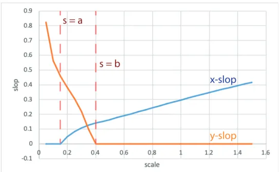
s = b

Figure 4.2.: Example of slop/extrinsic scatter (σx, σy) dependence on fitting scale s (for some linear

model). Note that as is predicted in_§3.0.3, there exist minimum and maximum scaless=a

ands=b(respectively) such that lim

s→a+σx= 0 and lim_s_→_b−σy = 0.

to find the two scale extrema at the same time using parallel computing (in the current,

C++ implementation of the TRK suite).

Now that the method for determining the scale extrema a and b for a certain model and

dataset has been presented, the optimum scales0 needs to be determined. From §3.0.3,

in order to determine successive approximations for s0 until convergence, Equation (3.6)

must be repeatedly solved for s(2)0 given the previous iteration’s solutions (1)

0 . I begin this process withs(1)₀ = (a+b)/2, and then successively solve Equation (3.6) numerically while

setting s(1)0 =s (2)

0 after each iteration.

In practice, Equation (3.6) is solved by rewriting it as

˜

RTRK2 (s (2) 0 ;s

(1)

0 , a, b)≡ 1 N N X n=1 tan2   π 4 − arctan

s(1)₀ tanθt,n;a

−arctans(1)₀ tanθ_s(2) 0 2   − 1 N N X n=1 tan2   π 4 − arctan

s(1)₀ tanθ_s(2) 0

−arctans(1)₀ tanθt,n;b

2  

= 0, (4.1)

and numerically solving the equation fors(2)0 given the previouss (1) 0 =s

(2)

(44)

Algorithm 5: Bracketing/Bisection-type method for determining minimum fitting scale a for some model and dataset.

1 Function FindMinimumScale

Input :Modelyc and dataset {xn, yn} with error bars {σx,n, σy,n}.

Output :Minimum fitting scalea.

2 begin

3 Determine brackets (l, r) for min scale a:

4 Initialize bisection brackets l=s= 0, r =s = 1 ands_trial =s= 1. 5 σx(strial)← DownhillSimplex(s=strial)

6 Initialize step modifierα = 0.5×strial. 7 if σ_x(s_trial)>0then

8 r=strial

9 l_trial =s_trial

10 σ_x(ltrial) =DownhillSimplex(s=ltrial) 11 while σx(ltrial)>0 do

12 l_trial =l_trial−α

13 σ_x(ltrial) =DownhillSimplex(s=ltrial) 14 α= 0.5×α

15 r=l_trial

16 end

17 l=l_trial

18 end

19 else if σ_x(s_trial) = 0 then 20 l=strial

21 r_trial =s_trial

22 σ_x(ltrial) =DownhillSimplex(s=ltrial) 23 while σx(rtrial) = 0 do

24 r_trial =r_trial+α

25 σ_x(rtrial) =DownhillSimplex(s=rtrial) 26 l=rtrial

27 end

28 r=r_trial

29 end

30 Use bisection to determine a now that we have brackets (l, r): 31 a_trial = (l+r)/2

32 σx(atrial) =DownhillSimplex(s =atrial)

33 while |l−r| ≥ tolerance1 AND σ_x(a_trial)≥ tolerance2 do 34 a_trial = (l+r)/2

35 σx(atrial) =DownhillSimplex(s=atrial)

36 if σ_x(a_trial)>0then 37 r=a_trial

38 end

39 else if σ_x(a_trial) = 0 then 40 l=a_trial

41 end

42 end

konz_thesis_draft_FINAL.pdf

Bayesian Model Fitting with Both Intrinsic and

Extrinsic Uncertainties in Two Dimensions

Nicholas Clayton Konz

Senior Honors Thesis

Department of Physics and Astronomy

The University of North Carolina at Chapel Hill

Acknowledgements

Contents

List of Figures

2.1. Statistical Preliminaries: Bayesian Statistics

2.2. Fitting a Model to Data in Two Dimensions

2.2.1. The Likelihood Function

y

(

x

;ϑ

)

x

y

x

y

y

(

((

x

;ϑ

)

y

y

((

;ϑ

;ϑ

σ

σ

σ

σ

σ

(

x , y

y

((

, y

, y

)))

σ

σ

σ

σ

σ

σ

2.2.2. An Analytical Approximation of the Likelihood

Σ

Σ

(

x

,

y

)

(

x

,

y

)

y

x

y

+

m

(

x-x

)

y

(

x

;

)

2.2.3. The TRK Likelihood

3. Properties of the TRK Statistic

3.0.1. Invertibility