0 Master’s Thesis Methodology and Statistics Master
Methodology and Statistics Unit, Institute of Psychology,
Faculty of Social and Behavioral Sciences, Leiden University
Date: July 2019
Student number: 1257285
Supervisor: Dr. M. Fokkema
Recursive partitioning of clustered data using LMM
trees: An empirical evaluation using educational data
Master’s Thesis
1
Content
Content ... 1
Abstract ... 2
Introduction ... 3
Multilevel data ... 3
Linear mixed-effects algorithm ... 4
Current study ... 4
Methods ... 5
Data. ... 5
Response variables ….. ... 6
Partitioning variables ... 6
Analysis ... 7
Results ... 9
Reading analysis ... 10
Conclusions of the reading analysis………. 11
Math analysis ... 12
Conclusions of the math analysis. ... 13
Discussion ... 14
Conclusion……….……… 14
Strengths and limitations ... 15
2
Abstract
Subgroup detection is an important aim in psychological research. Recursive partitioning methods allow for subgroup detection. Many datasets in the social sciences have a multilevel structure, where observations are clustered within higher-level units. For instance, students may be clustered within schools or classrooms. In such datasets, it can be expected that observations from the same cluster are more similar than observations from different clusters. In other words: the data is not independent of each other. Previous research suggested a recursive partitioning method that can take the clustering of data into account by allowing for the estimation of random effects: the linear mixed-effects tree (LMM).
The current study will evaluate the different ways to grow LMM trees. Specifically, the effects of using cluster-level parameter stability tests and initializing estimation with the estimation of random effects were assessed. This was assessed using data from the Early Childhood Longitudinal Study (ECLS) published by the National Centre for Education Studies (NCES, 2016). Four aspects were examined; predictive accuracy, tree size, variance of the random effects and the proportion of school-level variables in the trees.
The results showed that how to specify and partition LMM trees when potential
partitioning variables are measured at both the observation- and cluster-level depends on the
aim of the analysis. Trees should be grown using the default settings or the cluster argument
when the aim of the analysis is prediction. Trees that initialize estimation by estimating the
3
Introduction
Subgroup detection and prediction are important aims in psychological research. Lipkovich, Dmitrienko, Denne and Enas (2011) state that a common approach for the detection of subgroups used to be a linear regression-based analysis of subsets using models with main effects and interaction effects. They state that some of the downsides to this approach are low power and the need to specify the interaction terms and cut-off values a priori. A newer statistical approach that allows for subgroup detection are tree-based or recursive partitioning
methods. Lipkovich, Dmitrienko and D’Agostino (2017) describe a tree-based model as a
method that partitions the covariate space into rectangular areas or terminal nodes, in which
every subject is allocated to one of the terminal nodes, based on their covariate values. The
model will make certain splits based on the covariate values and can be regarded as a decision
model. Su, Tsai, Wang, Nickerson & Li (2009) explain that a tree is grown by looking for the
variable that can split the data into two groups with the greatest heterogeneity between the
newly formed groups compared to the other variables. This will also be done for the newly
created two groups and so on. To make a prediction for a new observation, the new
observation can be ‘dropped down’ the tree; the mean of the terminal node to which the
observation belongs is the predicted value for that subject. This recursive partitioning
procedure can be extended to accommodate a parametric model as well, instead of constant
fits in the nodes (Hothorn, Hornik & Zeileis, 2006).
Multilevel data
In many studies in psychological research the data being used has a multilevel structure, this
means that there will often be some sort of clustering. For instance: when data is collected
from children from different schools or from patients in different hospitals, the data points are
nested/clustered within the schools or within the hospitals. The observations from children
from the same schools or patients in the same hospital will be more alike than the
observations of children from different schools or patients from different hospitals. In other
words: the observations are not independent of each other. It is important to take such
clustering of the data into account, not doing so can lead to an overestimation of the
relationship between the variables and to choosing an overly complex model (Sela &
Simonof, 2012) as well as higher type-I error rates and possibly incorrect standard errors
4
Linear mixed-effects algorithm
Fokkema, Smits, Zeileis, Hothorn & Kelderman (2017) noted that most of the existing
tree-based algorithms were not able to take the clustering of data into account and proposed the
linear mixed-effects tree (LMM tree) algorithm to deal with this kind of data. The LMM
algorithm is based on an existing model based recursive partitioning method (MOB), allowing
for the estimation of linear model based recursive partitioning, as well as a global mixed- or
random-effects models (Fokkema et al., 2017). The LMM algorithm thus estimates random
effects to take the clustering into account. Zeileis, Hothorn and Hornik (2008) describe the
MOB algorithm, on which the LMM algorithm is based, as an algorithm that creates trees by
estimating a model for each node. To decide whether a node should be split, a statistical test
for parameter stability is performed. Once no further significant parameter instabilities are
found, the partitioning stops and the output will be a tree.
Fokkema et al. (2017) proposed the LMM algorithm and explained that it consists of
the following steps: First, a generalized linear tree (GLM tree) is estimated, with the random
effects set to zero for the first iteration. Second, a mixed-effects model is fit, using the
terminal nodes from the GLM tree, and the random-effects predictions are extracted. Note that
in this step, the random effects are estimated globally and the fixed effects are estimated
locally (within the terminal nodes). These two steps are repeated until the model converges.
The convergence of the model is monitored by computing the log-likelihood of the
mixed-effects model, estimated in the second step.
Fokkema et al. (2017) evaluated the algorithm by comparing it to various existing
methods and concluded that LMM trees may provide a promising tool for subgroup detection
for a broad range of prediction problems in multilevel data.
Current study
The original study from Fokkema et al. (2017) evaluated the LMM algorithm using simulated
clustered data. The current study will evaluate the LMM algorithm using data from an
existing educational dataset, with observations from children and their schools and teachers.
The observations of the children (observation-level) are clustered in the different schools
(cluster-level) and the outcome variables are the reading and mathematical abilities of the
children. The possible predictor variables consist of both observation- and cluster-level
variables. For instance, the gender of the children (observation-level) and the percentage of
male students for each school (cluster-level) are included.
5 uses parameter stability tests to check whether a split should be made. However, when dealing
with clustered data it is unclear whether these tests should be performed on the observation or
cluster level. Another uncertainty when using the LMM algorithm comes from the two steps
which are taken to create the trees, described above. The order in which the GLM and the
mixed-effects model are estimated can be switched around: estimation could initialize with
the tree structure, or with the random effects. It is yet uncertain which of these two
initialization approaches will perform best. To use the LMM algorithm in an optimal way,
these uncertainties should to be examined.
The main research question of the current study is: How should we specify and
partition linear-mixed model trees (LMM) when potential partitioning variables are measured
at both the observation- and cluster-level? To answer this question the LMM algorithm will
be evaluated on the following aspects: the differences when initializing estimation with the
random effects or the tree structure first and the differences between cluster-level parameter
stability tests and observation-level parameter stability tests. To evaluate performance, the
following outcomes will be assessed: the accuracy of the predictions in test data, the number
of nodes in the trees, the variance of the random effects and the level (observation or cluster)
of the selected predictor variables.
Methods Data
To answer the research question, data from the Early Childhood Longitudinal Study (ECLS) published by the National Centre for Education Studies was analysed (NCES, 2016). This
dataset consists of observations from students who started kindergarten in the academic year
of 1998-1999 in the United States. The students were followed from kindergarten through
eighth grade. The complete dataset consisted of 21,409 observations on 18,949 variables. The
current study used the data that was collected on the second measurement moment, this was in
the spring of the kindergarten year. The average age of all of the students in the complete
dataset from the second measurement moment was 6 years and 3 months (SD = 4.87
months). The possible predictor variables were chosen partly based on the study of Stegmann,
Jacobucci, Serang and Grimm (2018) and partly through our own interpretation. Two similar
analyses were performed; one to predict the reading scores and one to predict the mathematics
scores of the children. Because of the large number of observations, and because the function
6 deal with missing data. This resulted in a final datasets of 6,665 observations in the analysis
on reading scores and 7,591 observations in the analysis on the math scores.
Response variables
Reading score. The outcome variable that was chosen for the reading analysis was the
reading score of the children on the second measurement moment. This was a theta score
computed using Item Response Theory (IRT) modeling and ranged from -2.38 to 1.1. IRT is a
psychometric approach that takes the qualities of an individual and the qualities of the items
into account when looking at the response patterns (Furr & Bacharach, 2008).
Math score. The outcome variable for the analysis on mathematical ability was the
math score. This variable was also a theta score and ranged from -2.40 to 0.92.
Partitioning variables
Below, the possible partitioning variables used in the analyses are described. Some of the
variables were already in the original dataset, others were computed using variables in the
original dataset. Due to listwise deletion the same variables will have slightly different
distributions in the reading and math analyses.
Children and school identifiers. Child ID is the identification number for each child
in the study (child-level) and the School ID is the identification number of each school
(school-level). For the reading analysis there were 6,665 children from 928 different schools
in the dataset and for the math analysis there were 7,591 children from 1,001 different schools
in the dataset.
Gender. For both analyses the gender of the child (child-level) and the percentage of
male students per school (school-level) were used as potential predictor variables. For the
reading analysis, 50.32% of observations were male and 49.68% were female. For the math
analysis the observations consisted for 50.51% of male students and for 49.49% of female
students.
Race. The variable race was computed to have two categories: white and non-white.
Both the race of the child (child-level) and the percentage of white students per school
(school-level) were used as potential predictor variables. For the reading analysis 68.27% of
the students were white and 31.73% were non-white. For the math analysis, 65.68% of the
students were white and 34.32% of the student were non-white.
Socio-economic status. The variable socio-economic status on child-level was a
numerical variable ranging from -5 to 3, with higher values indicating a higher
7 per school (school-level) were used as potential predictor variables. For the reading analysis
the socio-economic status on the child-level had a mean of 0.20 (SD = 0.77) and for the math
analysis the mean was 0.15 (SD = 0.79) on the child-level.
Teacher certification. A variable indicating whether a teacher had regular/standard or
non-regular certification was created. For the reading analysis 82.45% of the teachers had a
standard certificate and 17.55% had a non-regular certificate. For the math analysis 82.18% of
the teachers had a standard certification and 17.82% had a non-regular certificate. For both
analyses, a school-level variable of certification was calculated reflecting the percentage of
teachers that had a regular certification of each school.
Reading at home. A variable about the contribution on the reading level of the child
by the parents was added for the analysis on reading ability. This variable consisted of how
often the parents would read to their children in a week. Of all of the children 0.75% didn’t
read with their parents at all, 14.25% read once or twice a week with their parents, 37.04%
read three to six times a week with their parents and 47.95% read every day with their parents.
Analysis
Software. The analyses were performed in R (R core team, 2018). The software that was used
to fit the LMM tree models was the R-package glmertree (Fokkema & Zeileis,2016). To test
for significant differences the R-package lmerTest was used (Kuznetsova, Brockhoff &
Christensen, 2017).
Model fitting. Four different tree-fitting approaches were used to fit a random
intercept model to the data, in all of them a random intercept was estimated with respect to the
School ID. The use of an intercept-only model resulted in a constant prediction for reading or
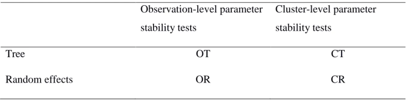
math score in each of the terminal nodes. Table 1 illustrates the design employed for fitting
the different trees.
The first tree-fitting approach can be seen as the default model. This means that
observation-level covariances were computed for the parameter stability tests. Also, model
estimation was initialized by fitting the tree, before estimating the random effects. This model
is referred to as the OT model.
The second tree-fitting approach was the same as the first approach, except that model
estimation was initialized by estimating the random effects, before growing the tree. This
tree-fitting approach is referred to as the OR model.
The third tree-fitting approach was the same as the first approach, except that
8 stability tests were performed at the school-, instead of the child-level. This can be done by
adding a cluster argument in the model specification when using the glmertree package. This
tree-fitting approach is referred to as the CT model.
The fourth tree-fitting approach was the combination of the second and third
approaches: it employed cluster-level parameter stability tests and initialized model
estimation with the random effects. This tree-fitting approach is referred to as the CR model.
Table 1. The different approaches used to create the trees.
Observation-level parameter
stability tests
Cluster-level parameter
stability tests
Tree OT CT
Random effects OR CR
Evaluation. The performance ofLMM trees was evaluated based on four outcomes:
Predictive accuracy: To guard against overfitting, the LMM trees were grown on one part of the dataset, and predictive accuracy was assessed on the remaining datapoints.
Specifically, 10 repeats of 10-fold cross validation were performed. To quantify predictive accuracy, the difference between the predicted and observed reading and math scores for the test observations were computed, and the mean squared error (MSE) was calculated for each tree-fitting approach (Table 1) in each of the 100 folds. To determine the folds for the cross validation, observation-level (not cluster-level) sampling was performed. To generate
predictions for new observations, only fixed-effects predictions (i.e., predictions from the
tree) were computed, the random effects were not included in the predictions.
Tree size: Tree size was evaluated by counting the number of nodes in each of the fitted trees.
Proportion of selected cluster-level variables: This was evaluated by calculating the proportion of school- and child-level variables appearing in each of the fitted trees.
Variance of the random effects: The estimated variance of the random effects was extracted from each fitted tree.
9
Results
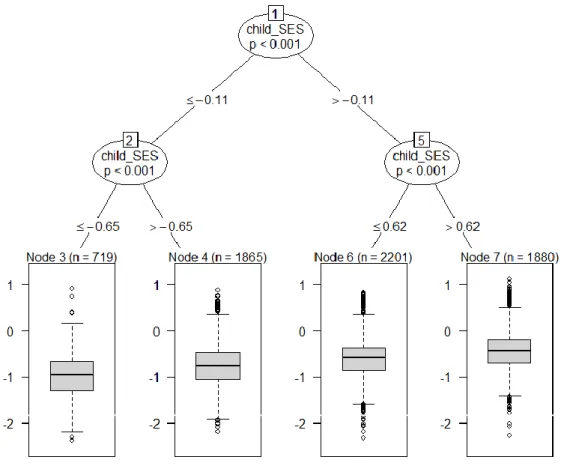
Figure 1 shows an example LMM tree that was grown for illustrative purposes. The
tree was grown using the default settings on the complete dataset with the reading scores as
the outcome variable, but with a maximum depth of three, to serve as an example. This tree
shows that the data was divided into four groups and the variable socio-ecomomic status of
the child (child_SES) was chosen all three times as the splitting variable. The tree had in total
seven nodes of which four were terminal nodes. Looking at the first split shows that the tree
divided the children into two different groups: children with a socio-economic status lower
than or equal to 0.11 and children with a status higher than 0.11. The terminal nodes show the
distribution of the children on the reading scores. An upwards trend in reading scores over the
four groups can be seen, revealing a positive association between reading skills and
socio-economic status. The variance of the random intercept with respect to school of the complete
dataset for this analysis was 0.035.
Figure SEQ Figure \* ARABIC 1. An example of a plot of a tree grown with the default settings.
10
Reading analysis
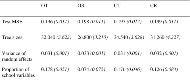
Table 2 shows the means and standard deviations of predictive accuracy, tree size, variance
of the random effects and proportion of selected school-level variables for the analysis on
reading scores, for all four different types of trees.
Table 2. Means and standard deviations (SD) of mean squared error (MSE) on test data, tree size, variance of the random intercept and the proportion of school-level variables for the analysis on reading scores.
Note. The means and standard deviations were calculated over the values per fold. The mean reading score was -0.646 (SD = 0.479).
Predictive accuracy. The first outcome that was evaluated was predictive accuracy.
Table 2 shows that the MSEs of the four different approaches to fitting the LMM trees gave
results that were close to each other. The trees that were grown using the default settings had
the lowest average MSE and the trees that initialized estimation with the random effects and
used the cluster argument had the highest average MSE. The standard deviations were very
similar. A one-way ANOVA showed that there was a significant difference between the types
of trees (F(3, 297) = 5.04, p < 0.01). Further inspection showed a significant difference
between the trees with the default settings and the trees that initialized estimation with the
random effects (t(297) = 1.98, p < 0.05) and the trees that used the cluster argument and that
initialized estimation with the random effects (t(297) = 3.76, p < 0.001).
Tree sizes. Table 2 shows that the trees that initialized estimation with the random
effects grew on average the smallest tree. The tree that used the cluster argument grew on
average the largest tree. A one-way ANOVA showed that there was a significant difference
between the types of trees (F(3, 297) = 101.39, p < 0.001). Further inspection showed a
significant difference between the trees with the default settings and the trees that initialized
estimation with the random effects (t(297) = -11.57, p < 0.001) and the trees that used the
OT OR CT CR
Test MSE 0.196 (0.011) 0.198 (0.011) 0.197 (0.012) 0.199 (0.011)
Tree sizes 32.040 (3.623) 26.800 (3.210) 34.540 (3.628) 31.260 (4.327)
Variance of random effects
0.031 (0.001) 0.033 (0.001) 0.031 (0.001) 0.032 (0.001)
Proportion of school variables
11 cluster argument (t(297) = 5.52, p < 0.001).
Variance of the random effects. The trees that initialized estimation by estimating
the random effects and the trees that used the cluster argument and initialized estimation with
the random effects had on average the highest variance of the random effects. All four
tree-growing methods had approximately similarly low standard deviations. A one-way ANOVA
showed a significant difference between the types of trees (F(3, 297) = 387.41, p < 0.001).
Further inspection showed a significant difference between the trees with the default settings
and the trees that initialized estimation with the random effects (t(297) = 27.25, p < 0.001)
and the trees that used the cluster argument and initialized estimation with the random effects
(t(297) = 21.94, p < 0.001).
Level of the selected splitting variables. The trees that initialized estimation with the
random effects selected the lowest number of school-level splitting variables. All four tree
types had low proportions; they selected more child-level variables as splitting variables. The
trees grown with the default settings had the highest proportion of school-level variables as
splitting variables. A one-way ANOVA showed a significant difference between the types of
trees (F(3, 297) = 80.04, p < 0.001). Further inspection showed a significant difference
between the trees with the default settings and the trees that initialized estimation with the
random effects (t(297) = -13.36, p < 0.001) and the trees that used the cluster argument and
that initialized estimation with the random effects (t(297) = -6.62, p < 0.001).
Conclusions of the reading analysis.
The values of the R2 for the four different types of trees ranged approximately from 0.133 to
0.146, with the higher values belonging to OT and CT trees. The intraclass correlation
coefficient (ICC) of the four different types of trees ranged approximately from 0.135 to
0.144, indicating that about 14% of variance in reading scores can be explained by school.
The higher values belonged to the OR and CR trees. The ICC and the R2 values indicate that
the tree and the random effects contribute similarly to the prediction of reading scores.
However, the ICC values were computed on training data, while the R2 values were computed
on test data.
The results showed that the predictive accuracy was significantly higher for the OR
and CR trees, when compared to the OT (default) trees. The smallest trees were grown by the
OR trees, this was a significant difference when compared to the OT (default) trees. The
variance of the random effects was significantly higher for the OR and CR trees when
12 selected as splitting variables in the OR and CR trees were significantly lower than for the OT
(default) trees.
Math analysis
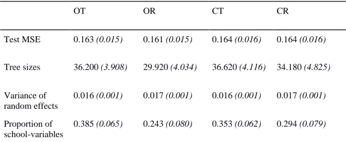
Table 3 shows the means and standard deviations of predictive accuracy, tree size, variance
of the random effects and proportion of school-level variables for the analysis on math scores.
Table 3. Means and standard deviations (SD) of mean squared error (MSE) on test data, tree size, variance of the random intercept and the proportion of school variables for the analysis on math scores.
OT OR CT CR
Test MSE 0.163 (0.015) 0.161 (0.015) 0.164 (0.016) 0.164 (0.016)
Tree sizes 36.200 (3.908) 29.920 (4.034) 36.620 (4.116) 34.180 (4.825)
Variance of random effects
0.016 (0.001) 0.017 (0.001) 0.016 (0.001) 0.017 (0.001)
Proportion of school-variables
0.385 (0.065) 0.243 (0.080) 0.353 (0.062) 0.294 (0.079)
Note. The means and standard deviations were calculated over the values per fold. The mean math score was -0.599 (SD = 0.448).
Predictive accuracy. The trees that used the cluster argument and the trees that used
the cluster argument and initialized estimation with the random effects had the highest MSE
on average. The tree that initialized estimation by estimating the random effects first had the
lowest MSE on average. A one-way ANOVA showed that there was not a significant
difference between the types of trees (F(3, 297) = 2.48, p = 0.061).
Tree sizes. Table 3 shows that the trees that initialized estimation with the random
effects had on average the lowest tree size. The tree that used the cluster argument grew on
average the largest tree. A one-way ANOVA showed a significant difference between the
types of trees (F(3, 297) = 86.75, p < 0.001). Further inspection showed a significant
difference between the trees with the default settings and the trees that initialized estimation
with the random effects (t(297) = -13.50, p < 0.001) and the trees that used the cluster
argument and initialized estimation with the random effects (t(297) = -4.34, p < 0.001).
Variance of the random effects. The trees that were grown using the default settings
and the trees that were grown using the cluster argument had on average the lowest variance
13 A one-way ANOVA showed a significant difference between the types of trees (F(3, 297) =
228.44, p < 0.001). Further inspection showed that the three other types of trees were
significantly higher than the trees with the default settings; the trees that initialized estimation
with the random effects (t(297) = 22.77, p < 0.001), the trees that used the cluster argument
(t(297) = 4.45, p < 0.001) and the trees that used the cluster argument and initialized
estimation with the random effects (t(297) = 17.34, p < 0.001).
Level of the selected splitting variables. The trees that initialized estimation by
estimating the random effects had the least school-level variables as selected splitting
variables. The trees with the default settings and trees with the cluster argument had the
largest proportion of school-level variables as splitting variables. A one-way ANOVA showed
a significant difference between the types of trees (F(3, 297) = 122.89, p < 0.001). Further
inspection showed a significant difference between the trees grown with the default settings
and all three of the other types of trees; the trees that initialized estimation with the random
effects (t(297) = -17.65, p < 0.001), trees with the cluster argument (t(297) = -3.96, p < 0.05)
and the trees that used the cluster argument and initialized estimation with the random effects
(t(297) = -11.35, p < 0.001).
Conclusions of the math analysis.
The values of the R2 for the four different types of trees ranged approximately from 0.183 to
0.198, which was higher than in the reading analyses. The OT and OR trees had the highest
R2 values. The ICC for the four different types of trees ranged approximately from 0.080 to
0.085, which was lower than in the reading analyses. The OR and CR trees had the highest
ICC values.
The results showed that predictive accuracy did not differ significantly between the
different trees. Both the CR and TR trees were significantly smaller than the OT (default)
trees. All three types of trees differed significantly from the trees that were grown using the
default settings in the variance of the random effects, they were all significantly higher. The
OT (default) trees selected the highest proportion of school-level variables as splitting
variables, followed by the CT, CR and OR trees, respectively, indicating that initializing
14
Discussion
Conclusion
The aim of the current study was to establish how we should specify and partition LMM trees
when potential partitioning variables are measured at both the observation- and cluster-level.
This was studied by looking at the possible differences when the estimation is initialized by
estimating the tree structure or estimating the random effects first and the possible differences
when parameter stability tests are performed on the observation- or cluster-level variables.
In terms of predictive accuracy we found that the OT and CT trees performed best
when predicting reading scores. No significant differences were found between the tree-fitting
approaches in predicting math scores.
In terms of tree size, we found that both the OR and CR trees were the least complex
for predicting both reading and math scores. This means that when growing a tree by
initializing estimation with the random effects, with or without the use of the cluster
argument, there are less splits needed for the model to converge. In other words these types of
trees need less splits to find the best fitting models.
The variances of the random effects were significantly higher for the OR and CR trees
compared to the OT (default) trees. In other words, initializing estimation with the random
effects yielded higher ICC values.
The proportion of school-level variables as selected splitting variables was low in both
analyses. The OR and CR trees had significantly less school-level variables as splitting
variables. For the analysis of mathematical ability a significant difference was also found for
the CT trees when compared to the trees that were grown using the default settings. This
shows that when initializing estimation with the random effects, the lowest number of
school-level variables are chosen as partitioning variables.
Based on these findings we can conclude that there is not an overall best way to
specify and partition LMM trees when potential partitioning variables are measured at both
the observation- and cluster-level. The right answer to what the best way to specify LMM
trees is, may depend on the aim of the analysis. When the aim is to obtain accurate predictions
for the outcome variable, the trees can be grown using the default settings, or using the cluster
argument. When the aim is to obtain a less complex tree, the tree that initializes estimation
with the random effects but does not use the cluster argument should be used. The results also
show that when initializing estimation with the random effects, the variance of the random
15 of the random effects are larger, the ICC will become larger as well and thus will show that
more variance on the cluster-level is accounted for by the random effects. When initializing
estimation with the tree structure, more variance on the cluster-level is accounted for by the
tree because more cluster-level splitting variables are selected.
Strengths and limitations
The current study contains some strengths and limitations. The first limitation is that it is not possible to know the true model if real-world datasets are analysed. This means that we do not know whether a tree has spurious splits or is missing splits. Based on the results of the current study we only know that there is one of the four types of trees that creates the smallest tree, but it is possible that this tree is missing important splits. A strength is that we performed analyses on two different response variables, which may make the results more generalizable to other real-world datasets. A possible way to check if the tree-fitting approaches can recover subgroups and effects which are known to be present in the data, could be to use simulated data. Fokkema et al. (2017) used simulated data to check whether the LMM tree algorithm could recreate the actual tree. This same approach could be used to check if the four different tree-fitting approaches perform equally well or different when attempting to recover the actual tree.
The second limitation is the use of listwise deletion instead of, for instance, multiple imputation. The LMM tree algorithm cannot deal with missing data, as a way of dealing with the missing data listwise deletion was chosen. The listwise deletion was seen as an option because of the large number of datapoints in the dataset. However, it is possible that entire schools, with possibly different response patterns, were excluded because there were no students from that school with complete observations. Because of the deletion of students with incomplete responses these schools are not taken into account when constructing the model. This can lead to a different conclusion compared to when they would have been included during the estimation of the model. However, even with the use of listwise deletion a large number of observations were left in the dataset for both analyses. To guard against overfitting and to increase the generalizability of the results to other datasets even more, 10 repeats of 10-fold cross-validation were performed.
16
groups are approximately twice as large as the number of groups in the study of Theall et al. (2011), so we can assume that the estimates are not affected by the small group sizes.
To conclude, the current study shows the differences between four different tree-fitting
approaches when potential partitioning variables are measured at both the observation- and
cluster-level and states some potential improvements for future studies about subgroup
17
Literature
Furr, R.M. & Bacharach, V.R. (2008). Psychometrics: an introduction. Thousand Oaks, CA;
Sage Publications, Inc.
Fokkema, M, Smits, N., Zeileis, A., Hothorn, T. & Kelderman, H. (2017). Detecting
treatment-subgroup interactions in clustered data with generalized linear
mixed-effects model trees. Behavior Research Methods. doi:10.3758/s13428-017-0971-x
Fokkema, M., & Zeileis, A. (2016). glmertree: Generalized linear mixed model trees.
Retrieved from http://R-Forge.R-project.org/R/?group id=261 (R package version
0.1.2)
Hothorn, T., Hornik, K., & Zeileis, A. (2006). Unbiased recursive partitioning: A
conditional inference framework. Journal of Computational and Graphical
statistics, 15(3), 651- 674.
Kuznetsova A, Brockhoff P.B. & Christensen, R.H.B. (2017). lmerTest Package: Tests in
Linear Mixed Effects Models. Retrieved from
https://github.com/runehaubo/lmerTestR (R package version 3.1.0)
Lipkovich, I., Dmitrienko, A. & D’Agostino SR., R.B. (2017). Tutorial in biostatistics:
data-driven subgroup identification and analysis in clinical trials. Statistics in Medicine,
36(1), 136-196.
Lipkovich, I., Dmitrienko, A., Denne, J., & Enas, G. (2011). Subgroup identification based
on differential effect search - A recursive partitioning method for establishing
response to treatment in patient subpopulations. Statistics in Medicine, 30(21), 2601–
2621.
National Center for Education Statistics. (2016). Early Childhood Longitudinal Program:
Kindergarten class of 1998–1999 (ECLS-K) [Data file]. Available from National
Center for Education Statistics site: https://nces.ed.gov/ecls/kindergarten.asp.
R Core Team (2018). R: A language and environment for statistical computing. R Foundation
for Statistical Computing, Vienna, Austria. URL https://www.R-project.org/.
Sela, R.J. & Simonoff, J.S. (2012). RE-EM trees: a data mining approach for longitudinal
18 Su, X., Tsai, C., Wang, H., Nickerson, D.M. & Li, B. (2009) Subgroup analysis via
recursive partitioning. Journal of Machine Learning Research, 10, 141-158.
Steenbergen, M.R. & Jones, B.S. (2002). Modeling multilevel data structures. American
Journal of Political Science, 46(1), 218-237.
Stegmann, G., Jacobucci, R., Serang, S. & Grimm, K.J. (2018). Recursive partitioning with
nonlinear models of change. Multivariate Behavioral Research, 53(4), 559-570.
Theall, P.K., Schribner, R., Broyles, S., Yu, Q., Chotalia, J., Simonsen, N., Schonlau, M. &
Corlin, B.P. (2011). Impact of small group size on neighborhood influences in
multilevel models. Journal of Epidemioly Community Health, 65(8), 688-695.
Zeileis, A., Hothorn, T. & Hornik, K. (2008). Model-Based Recursive Partitioning. Journal of