1703.02981.pdf

(1)

6D SCFTs and Phases of 5D Theories

Michele Del Zotto

1∗

, Jonathan J. Heckman

2†

, and David R. Morrison

3,4‡

1_{Simons Center for Geometry and Physics, Stony Brook, NY 11794, USA} 2_{Department of Physics, University of North Carolina, Chapel Hill, NC 27599, USA} 3_{Department of Mathematics, University of California Santa Barbara, CA 93106, USA}

4_{Department of Physics, University of California Santa Barbara, CA 93106, USA}

Abstract

Starting from 6D superconformal field theories (SCFTs) realized via F-theory, we show how reduction on a circle leads to a uniform perspective on the phase structure of the resulting 5D theories, and their possible conformal fixed points. Using the correspondence between F-theory reduced on a circle and M-theory on the corresponding elliptically fibered Calabi–Yau threefold, we show that each 6D SCFT with minimal supersymmetry directly reduces to a collection of between one and four 5D SCFTs. Additionally, we find that in most cases, reduction of the tensor branch of a 6D SCFT yields a 5D generalization of a quiver gauge theory. These two reductions of the theory often correspond to different phases in the 5D theory which are in general connected by a sequence of flop transitions in the extended K¨ahler cone of the Calabi–Yau threefold. We also elaborate on the structure of the resulting conformal fixed points, and emergent flavor symmetries, as realized by M-theory on a canonical singularity.

March 2017

∗_e-mail: _{[email protected]} †_e-mail: _{[email protected]}

‡_e-mail: _{[email protected]}

(2)

1 Introduction

Developing tools to characterize interacting SCFTs in higher spacetime dimensions is one of the challenges of contemporary theoretical physics. These systems exhibit striking departures from the standard paradigm of lower dimensional examples. The traditional methods of perturbation theory do not apply, and one must instead resort to stringy constructions to even establish existence. One of the remarkable recent developments in string theory is that not only do such theories exist, but many of their properties can be understood by using the geometry of extra dimensions.

Celebrated examples of this type are 6D superconformal field theories (SCFTs) [1–3]. For theories with (2,0) supersymmetry, there is an ADE classification given by Type IIB on supersymmetric orbifolds _C2_/_Γ

ADE (see also [4–6]). For theories with (1,0) supersymmetry, there is a related classification of the theories which can be obtained from F-theory [7–13]. Several features of these models are captured by the above string constructions, for instance the moduli spaces of vacua are captured by deformations of the Calabi–Yau geometry, the anomaly polynomials are encoded in the intersection theory of the F-theory base [14–16], and the 6D omega-background partition function is captured by topological string amplitudes on the Calabi–Yau (see e.g. [17–21]).

Compactification also yields insight into strongly coupled phases of lower-dimensional systems. For example, in the case of the 6D theories with (2,0) supersymmetry, the higher-dimensional perspective provides a geometric origin for non-trivial 4D dualities [22–25]. Though there is reduced supersymmetry in the case of the 6D (1,0) theories, there has recently been significant progress in developing analogous results [26–38].

Our aim in this work will be to use this 6D perspective to shed light on the phase structure of 5D field theories. For earlier work on the construction and study of such theories, see for example, [39–43], and for more recent studies, see for example [44–51]. Stringy constructions of such 5D fixed points include D-brane probes of singularities [52], suspended (p, q) five-brane webs [53,54], and purely geometric realizations using M-theory on a Calabi– Yau threefold with a canonical singularity [39, 41, 55, 56, 42, 57].

One of the confusing issues in such 5D theories is the existence of rather tight constraints on purely gauge theoretic constructions. Using only effective field theory arguments, refer-ence [42] argued that the strong coupling limit of a 5D gauge theory can only produce a conformal fixed point when there is a single simple gauge group factor, with a strict upper bound on the total number of flavors (i.e., weakly coupled hypermultiplets). This comes about because in five dimensions, supersymmetry constrains the metric on the Coulomb branch moduli space. To reach a conformal fixed point (starting from a gauge theory), we need to be able to reach the singular regions of moduli space, but having more than one gauge group factor obstructs this limit.

(4)

often take the form of a quiver gauge theory, i.e., a gauge theory of precisely the type ruled out by reference [42]. The key loophole [53,44] is that by moving in the vacuum moduli space of the 6D SCFT compactified on S1_{, one may reach points at which the effective 5D theory} is superconformal. While moving in the moduli space, one may reach a region in which the inverse gauge coupling squared of the field theory is formally negative. Before reaching such a region, the effective field theory description which had been valid in the gauge theory region breaks down and undergoes a phase transition. While such an operation is ill-defined in gauge theory, it has a well-known meaning in Calabi–Yau geometry: It is a flop transition! In M-theory compactified on a Calabi–Yau threefold, flopping a curve formally means we continue its area to a negative value. What is really happening is that we pass from one chamber of K¨ahler moduli space to another and the curve being flopped is the one whose area controls the value of the inverse gauge coupling squared. In the flopped phase we get another Calabi–Yau geometry. In the 5D SCFT literature this is sometimes referred to as a “UV duality,” though we shall avoid this terminology.

In this paper we study the phase structure of 5D theories which descend from compacti-fication of a 6D SCFT or its deformations. For some preliminary analyses of these theories, see e.g. [30, 33, 39]. One of the general lessons from [12] is that an appropriate partial tensor branch of a 6D SCFT is just a generalization of a quiver gauge theory in which the link fields are themselves strongly coupled 6D SCFTs. Geometrically, the tensor branch is obtained by performing a partial resolution of collapsing curves in the base of the elliptic fibration. Starting from this partial tensor branch, reduction on a circle takes us to a generalization of a 5D quiver gauge theory. Alternatively, we can remain at the 6D fixed point and reduce on a circle. For (1,0) theories, we find that this always yields a 5D SCFT, or more precisely, a collection of between one and four 5D SCFTs.

Our primary claim is that these two 5D theories are connected by a path in moduli space which is in general realized by a sequence of flop transitions. To see this, note that F-theory compactified on an elliptic Calabi–Yau threefold is, under reduction on a further circle, described by M-theory on the same Calabi–Yau threefold [58–60].1 In the M-theory description, the volumeVE of the elliptic fiber is related to the radius RS1 of the circle as:

VE = 1/RS1. (1.1)

Compactification on a circle of the 6D tensor branch theory is realized by first resolving the base of the F-theory model, and then resolving the elliptic fiber, taking it to infinite size. Compactification of the 6D SCFT is realized by only resolving the elliptic fiber taking it to infinite size. From the geometric engineering perspective, the latter possibility gives rise to a 5D SCFT because we automatically have divisors collapsed to points. However, the geometry also indicates that the former is indeed a phase connected to the 5D SCFT. We

1_{In what follows we shall always assume a Kaluza-Klein reduction on the circle in which we do not}

(5)

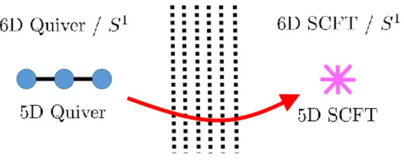
Figure 1: Depiction of the phase structure for 6D theories reduced on a circle. Reducing a (1,0) 6D SCFT leads to a 5D SCFT, as indicated on the right. A sequence of flop transitions in the extended K¨ahler cone of the Calabi–Yau threefold connects this chamber of moduli space to the one obtained by dimensional reduction of the generalized 6D quiver. This leads to a generalized 5D quiver, which need not possess a fixed point in this chamber of moduli space.

give a conceptual depiction of this trajectory in Figure 1.

So, whereas compactification of the 6D SCFT generates a 5D SCFT, the generalized quiver will not necessarily lead directly to a 5D SCFT. Rather, one must consider a motion in the extended K¨ahler cone of the Calabi–Yau threefold. The existence of the F-theory model is what guarantees that such a motion in moduli space is possible, and does indeed lead to a non-trivial 5D fixed point.

We stress that the moduli space for M-theory on a CY three-fold used in a geometric engineering of a 6D SCFT within F-theory is strictly larger than the moduli space of a 5D SCFT: indeed, it equals the moduli space of the 6D SCFT compactified on S1_{. To} obtain the moduli space of the 5D SCFT, the radius of the circle must be taken to zero size. Correspondingly, VE must be taken to infinity. There are different inequivalent limits

in which the volume of the elliptic fiber is sent to infinity, leading to different 5D fixed points. This is somewhat reminiscent of what happens for 6D little string theories, that admit various inequivalent decoupling limits, leading to distinct 6D SCFTs [61].

From the perspective of M-theory compactified on a non-compact Calabi–Yau threefold, generating a 5D SCFT simply requires that some divisors simultaneously collapse to a point at some location in the moduli space. There can be multiple such locations, possibly located in distinct phase regions.

Of course, the above remarks prompt the question as to what fixed point is actually realized by compactifying a 6D SCFT on a circle. Geometrically, we characterize this singular limit by F-theory on a base_C2_/_Γ

(6)

subgroups lead to a consistent base for an F-theory model, and have been classified in [7] (see also [35]). Making such a choice, we construct a Weierstrass model:

y2 =x3+f x+g, (1.2) where here, f and g are polynomials in the holomorphic coordinates of _C2 _{which transform} equivariantly under the action by the group ΓU(2). The order of vanishing forf andgdictates the enhancement for elliptic fibrations. This characterization provides a direct way to access the 5D fixed point: Since we have not performed any resolutions in the base, the only thing left for us to do is take the limit where the elliptic fiber class expands to infinite size while remaining maximally singular.2 In this limit, we find that the 5D theory breaks up into at most four decoupled SCFTs. In particular, the number of such constituent 5D SCFTs is much smaller than the dimension of the tensor branch for the 6D SCFT. Some of these constituents correspond to supersymmetric orbifold singularities of the form _C3_/_Γ

SU(3) for ΓSU(3) a finite subgroup of SU(3). There is typically another constituent corresponding to collapsing a collection of four-cycles to a non-orbifold singularity.

To illustrate these points, we also present a number of concrete examples. Perhaps the simplest class of examples are those where the ΓU(2)-equivariant polynomials f and g of equation (1.2) are generic, i.e., no tuning is performed. These were referred to as “rigid theories” in reference [7]. For these theories, we can fully characterize the resulting 5D fixed point just using the data of ΓU(2) itself. Further tuning leads us to additional examples of generalized quivers, some of which admit a rather simple form in F-theory. All of these cases lead to novel generalized quiver gauge theories in five dimensions, and the F-theory model serves to specify a path in moduli space to a fixed point after several flops.

The rest of this paper is organized as follows. First, in section 2 we give a general review of how to generate 5D SCFTs from compactifications of M-theory on a non-compact Calabi– Yau threefold. After this, we turn in section 3 to a brief review of the construction of 6D SCFTs via F-theory, emphasizing the particular role of the orbifold singularity in the base. We next turn in section 4 to an analysis of the 5D effective theories obtained by directly compactifying a 6D SCFT on a circle, as well as the compactification of its tensor branch deformation. We illustrate these general points with specific examples in section 5, and present our conclusions and some directions for future work in section 6. Additional details on the phases of the simple rank one non-Higgsable clusters are presented in Appendix A.

As this paper neared completion, we received [62] which considers a number of the same examples. See also [63].

2_{Naively, we can think of a given singular elliptic fiber as if it corresponds to an affine ADE graph}

(7)

2 5D SCFTs from M-theory

In preparation for our analysis of 6D theories compactified on a circle, in this section we review the construction of 5D SCFTs via M-theory on a (non-compact) Calabi–Yau threefold

X.3 _{To realize an interacting fixed point we need to reach a singular limit in Calabi–Yau} moduli space, which we expect to be resolved in the physical theory by the presence of additional massless / tensionless states. Said differently, we expect 5D SCFTs for M-theory on any canonical singularity P ∈Xsing with a crepant resolution (i.e., Calabi–Yau blowup)

π:X →Xsing which includes curve(s) and divisor(s) in the inverse image π−1(P) [42]. The geometric method we present subsumes other methods such as the construction of 5D SCFTs via webs of (p, q) five-branes in type IIB string theory. Indeed, as is well-known, each of these web diagrams also defines a toric Calabi–Yau threefold [67]. The conformal limit in such constructions involves bringing the various filaments of the web to the same location in the web, i.e., a singular point, and in the interacting case always involves some compact face of the (p, q) web collapsing to zero size. In toric geometry, such faces are interpreted as compact divisors, and the limit where the face degenerates to zero size at a single point simply corresponds to the contraction of this divisor to a point.

Let us now turn to the construction of M-theory on a canonical singularity and explain in more general terms why we expect to realize 5D SCFTs. To see why, recall that we measure volumes of even-dimensional cycles by integrating powers of the K¨ahler formJ. For example, for a two-cycle C, the volume is:

Vol(C) =

Z

C

J. (2.1)

For an M2-brane wrapped over a two-cycle, we get a BPS particle with mass proportional to this volume. For an M5-brane wrapped over a divisor, we get a BPS string with tension specified by the volume of this divisor. In the limit where the volume of the divisor passes to zero, this tension drops to zero. A priori, the region in moduli space where particles become massless and strings become tensionless can be different [68].

Now, to generate an interacting fixed point, we require at least one non-trivial divisor to collapse to a point in the geometry. The reason is that with just collapsing curves, we only obtain some collection of free hypermultiplets whereas with divisors collapsing to a curve, we get nonabelian gauge symmetry rather than an interacting fixed point. Assuming, then, that we have at least one collapsing divisor, our task reduces to determining possible connected configurations of curves and divisors which can all collapse simultaneously to a single point. A necessary and sufficient condition for arranging this is to require first of all, that we have a non-compact Calabi–Yau with a complete metric (i.e., we can decouple gravity), and second of all, that the metric on the K¨ahler moduli space remains positive definite as we pass to the putative singular point of moduli space.

(8)

For M-theory on a compact Calabi–Yau threefoldX withh1,1 _K¨_{ahler moduli, if we choose} a basis DI ∈Hcpt1,1(X), then the K¨ahler form is given by

J =

h1,1

X

I=1

mIDI. (2.2)

Scaling the K¨ahler class does not change the M-theory moduli, so the K¨ahler moduli are usually expressed as the “volume one locus” within H1,1₍_X_{), namely we use effective} coor-dinates

ϕI ≡mI/V1/3, I = 1, ..., h1,1 −1 (2.3)

whereV ≡ 1 3!

R

XJ∧J∧J. In practice we can scale V to infinity and simultaneously rescale

the mI _{in such a way that}

ϕI =

Z

CI

J, I = 1, ..., h1,1−1 (2.4)

remains finite and possibly non-zero. Here, CI is a the basis of dual compact 2-cycles. An

M2-brane wrapped over such a curve yields a BPS particle with mass specified by ϕI. The bosonic superpartners of ϕ define abelian vector bosons, which we denote by AI_{. They are}

given by integrating the three-form potential of M-theory over the same two-cycles:

AI =

Z

C

C(3). (2.5)

Similarly, one can introduce dual coordinates ϕI ≡ DIJ KϕJϕK where DIJ K is the triple

intersection number of X, that controls the size of a basis of four-cycles of X. The ϕI _are

the coordinates along the Coulomb phase which control the masses of BPS particles for the 5D theory, while the ϕI are the dual coordinates, which control the tensions of the BPS

monopole strings of the 5D theory.

The moduli space of M-theory on X is given by the extended K¨ahler cone of X [39]. A wall for a chamber of moduli space C is defined by the condition that either (1) a curve shrinks to a point or a divisor shrinks to (2) a curve or (3) a point. For a given chamber C, the effective action for these abelian vector multiplets is controlled by the 5D prepotential. Its form is given by a cubic polynomial in the K¨ahler moduli:

FC =

1

3!DIJ Kϕ

I

ϕJϕK, (2.6)

where the DIJ K are given by the triple intersection numbers for divisors in the Calabi–Yau

threefold:

(9)

From this, we can read off the metric on moduli space:

GIJ =

∂2_F

C

∂ϕI_∂ϕJ. (2.8)

Indeed, the low energy effective action contains h1,1 −1 5D abelian vector multiplets with couplings (see e.g. [42]):

Leff =GIJdϕI∧ ∗dϕJ +GIJFI∧ ∗FJ +

DIJ K

24π2A

I_∧

FJ∧FK+· · · (2.9)

where here, FI ₌_dAI _{is the field strength for the vector boson.}

Now, to reach a conformal fixed point, it is necessary for us to move to a singular region of the geometry. So, we select some subset of theϕI, which we denote by the restricted index

ϕi. We then hold fixed the remaining K¨ahler moduli so that, for example, derivatives of the prepotential with respect to these moduli are set to zero. Gij gives the matrix of effective

gauge couplings, and with respect to this subset, we demand that the Gij is positive away

from the origin. When this condition is satisfied, we can collapse the associated four-cycles to zero size, and we thus expect to realize a 5D SCFT. When this condition is not satisfied, we cannot simultaneously contract the size of all of the divisors. From this perspective, the task of determining candidate SCFTs from M-theory configurations involves analyzing all possible choices of divisors subject to these criteria. This condition of positivity as we move to the origin of moduli space can also be stated as a convexity condition on our prepotential [42]:

FC(λ(1)ϕ

i

(1)+λ(2)ϕi(2))≤ FC(λ(1)ϕ

i

(1)) +FC(λ(2)ϕi(2)) (2.10) with:

λ(1)+λ(2) = 1 and 0≤λ(1), λ(2) ≤1. (2.11) If we cannot satisfy this criterion, then we conclude that it is not possible to reach a conformal fixed point in a particular chamber.

In such situations, we can of course, also contemplate formally continuing some of the parametersϕIto negative values, i.e., we allow negative area for a given curve. Geometrically this is described by a flop transition between two Calabi–Yau manifolds with the same Hodge numbers. In this flopped phase, the structure of the triple intersection numbers will change, and consequently, also the prepotential. Observe that an M2-brane wrapped on such a curve will generate a BPS state with mass which goes from being positive to negative.4 _{Once we} have the new triple intersection numbers, we can again analyze whether the prepotential is convex in the new chamber Cnew. An important feature of the new prepotential is that it retains much of the structure of the original. To exhibit this, we view FC as a function of

4_{Many flop transitions can be thought of as being realized by replacing a given curve with normal bundle}

either O(−1)⊕ O(−1) or O ⊕ O(−2) with an F1 which is then shrunk down with respect to the other

(10)

positive values for the moduli|ϕi_|_{. The change between the prepotential for the old and new}

phase can be written in the form

Fnew− Fold=

1 3!L

3

, (2.12)

whereL= (P

mI_D

I)·Cflopis a linear function vanishing on the wall between the two K¨ahler cones which is positive after the flop [75, 41].

An interesting open question is to provide an explicit classification of all canonical sin-gularities which can generate 5D SCFTs. Compared with the classification strategy for 6D SCFTs generated by F-theory [7, 12], this is a far more intricate question because it involves tracking the collapse of four-cycles in our geometry. For example, we generate canonical sin-gualarities from the orbifolds_C3_/_Γ

SU(3) with ΓSU(3) a finite subgroup ofSU(3). The resolved geometry will typically contain multiple divisors all collapsing to zero size simultaneously. There can also be various intermediate limits where a K¨ahler surface first collapses to a curve, and then this curve futher degenerates to a point. In some cases, this degeneration has an interpretation in terms of 5D gauge theory, though in most cases it is more “exotic” from the perspective of effective field theory.

Our plan in the rest of this section will be to illustrate some of these considerations for a few well known examples. We will then proceed in the following sections to a much broader class of examples as engineered by compactifications of 6D SCFTs on a circle.

2.1 Single Divisor Theories

In this subsection we consider 5D SCFTs generated by a single collapsing divisor in a Calabi– Yau threefold. Assuming that the normal geometry in the Calabi–Yau threefold is smooth, we can locally characterize the geometry by the total space O(KS)→S, with S the K¨ahler

surface. The triple intersection number for the divisor S can also be evaluated using inter-section theory on the surface itself. Indeed, we have:

S·CYS·CYS =KS·S KS, (2.13)

where the subscripts for ·CY and ·S indicate that the intersection takes place in the

corre-sponding K¨ahler manifold. A necessary condition to reach a conformal fixed point is that the metric on the moduli space remains positive definite, so we must require:

KS·KS >0. (2.14)

This condition is somewhat milder than the condition that we can directly contract S to a point. Indeed, to decouple gravity in a local M-theory model, we either requireS to contract to a point, or to a curve. In the former case, we impose the stronger condition −KS > 0,

(11)

is satisfied, for example, for the Hirzebruch surfaces _Fn, with n ≥ 2 (which are not Fano).

Observe that condition (2.14) is not satisfied for a del Pezzo 9 (i.e., half K3) or K3 surface. Now, in the case of the del Pezzok surfacesdPk, i.e.,P2 blown up at a 0≤k ≤8 points, there is a well known correspondence for k ≥ 1 to a 5D SU(2) gauge theory with k −1 hypermultiplets. In this geometric picture, the SU(2) gauge theory is realized by noting that each del Pezzo surface can also be viewed as a _P1

fiber bundle over a P1base, possibly with some locations where this fibration degenerates. In the limit where the fiber_P1_fibercollapses to zero size, we get a curve of A1 singularities, realizing an SU(2) gauge theory. The locations where the fibration degenerates lead to local enhancements in the singularity type, providing additional matter fields [41,55]. The casek = 0 does not admit an interpretation as anSU(2) gauge theory, but is instead known as the “E0 theory,” (or C3/Z3) as in reference [41]. In all cases, we reach a conformal fixed point by collapsing the K¨ahler surface to a point. This also leads to an enhancement in the flavor symmetry, which can be directly computed via the geometry [41]. It is given by the exceptional groupEk, where fork <6 we simply delete

appropriate nodes from the affine Dynkin diagram Eb8.

A more unified perspective on all of these examples comes from first starting with the local geometry defined by a del Pezzo nine surface [60, 41]. This can be viewed as _P2 _blown up at nine points, and is also described by a Weierstrass model of the form:

y2 =x3+f4x+g6, (2.15) namely, we have an elliptic fibration over a_P1 _{in which the Weierstrass coefficients}_f

4 andg6 are respectively degree four and six homogeneous polynomials. Flopping the zero section of this model, we then blow down additional points to reach the various del Pezzo models. These correspond in the field theory to adding mass deformations to the associated hypermultiplets. An additional class of examples are given by the Hirzebruch surfaces _Fn, which forn >1

are not Fano, i.e., −KS is not positive. From the perspective of the M-theory construction,

we cannot construct a local metric which is complete. From a field theory point of view, this is the statement that there is no way to fully decouple gravity. Rather, we must include some additional degrees of freedom to complete the description. In the geometry, this requires us to introduce some additional divisors. Assuming the existence of at least one more divisor, we can now see why such a model could produce a 5D SCFT. First of all, we recall that Fn can also be viewed as a P1fiber bundle over a P

1

base, in which the first Chern class of the bundle is n. If we can take a limit in the Calabi–Yau moduli space in which the volume of P1base collapses to zero size, we get a weighted projective spaceP2[1,1,n]. This can then collapse to zero size. Of course, this assumes that we can collapse the _P1

(12)

2.2 Quiver Gauge Theories

So far, we have focussed on the geometric construction of 5D SCFTs. One can also attempt to engineer examples using methods from low energy effective field theory. Along these lines, we can consider a 5D quiver gauge theory with simple gauge group factorsG1, ..., Gl, and with

matter fields in some representation between these gauge group factors, i.e., hypermultiplets in bifundamental representations (Ri, Rj). The construction of such models is concisely

summarized by a quiver diagram.

Geometrically, we engineer a 5D gauge theory with gauge group G by introducing a curve of singularities. Locally, these are described by specifying a curve, and then taking a fibration by a space _C2_/_Γ

ADE with ΓADE a discrete subgroup ofSU(2) [76]. This yields the ADE groups, and the non-simply laced algebras can also be realized by allowing suitable monodromies in the fibration [77]. In these models, the value of the gauge coupling is controlled by the volume of the base curve. We can also engineer matter fields by introducing local enhancements in the singularity type of the fibration [78].

Collisions between curves supporting gauge groups can also produce a strongly coupled version of a hypermultiplet which is the 5D version of 6D conformal matter [11]. Some canonical examples of such behavior include the reduction of 6D conformal matter on a circle, a point we return to shortly. In five dimensions one can also contemplate more intricate intersection patterns, leading to further generalizations for 5D conformal matter.

Using methods either from gauge theory and/or geometry, it is possible to calculate the prepotential for these sorts of models. A perhaps surprising feature of all of these cases is that only for a single simple gauge group factor do we have a chance of realizing a 5D SCFT connected to every chamber of moduli space [42]. The reason for this is clear from the structure of the prepotential F, which contains a term of the schematic form:

− 1

12|cϕ+ϕ

0_|3

, (2.16)

whereϕis the Coulomb branch parameter(s) associated with one simple gauge group factor, and ϕ0 are associated with other Coulomb branch parameters. Physically, the vevs ofϕ0 can be viewed as giving masses to some of the hypermultiplets. The issue is that the contribution from such a term violates the convexity condition of line (2.10). Indeed, in the geometry, what is happening is that a curve C in a surface S is collapsing to zero volume before that surface can pass to zero volume as well. To continue the contraction of the surface, it is thus necessary to assume that we can continue the volume ofC to formally negative values, i.e., we must require the existence of a flop transition, bringing us to a different chamber of moduli space.5

5_{As an example of this type, ref. [53] considers a (}_{p, q}_{)-fivebrane web construction of}_SU₍₂₎_×_SU_{(2) gauge}

(13)

Without further input, we cannot conclude whether it is possible to reach a 5D SCFT through a sequence of flops. What we can conclude, however, is that in the chamber of moduli space where a quiver gauge theory description is valid, we do not expect to reach a 5D SCFT. One of our aims in this paper will be to elaborate on when we expect to achieve a sequence of flop transitions to a chamber which supports a 5D SCFT.

In the case of 6D theories on S1 _{the existence of such chamber is guaranteed from the} existence of the 6D fixed point. To gain further insight into the structure of possible 5D SCFTs, we shall use this higher-dimensional perspective. This will help us in determining candidate 5D theories, as well as establishing the existence of flops between these models.

2.3 M-theory on an Elliptic Calabi–Yau Threefold

When approaching the construction of 5D SCFTs from a 6D origin, we must consider M-theory on an elliptic Calabi–Yau threefold. The threefold need not be compact, but it should contain compact elliptic curves.

Specifically, we consider a proper6 map π : X → B from a (non-compact) Calabi–Yau threefold to a (non-compact) surface B whose general fiber is a compact elliptic curve. We assume that there is a birational section7 _{of this fibration} _σ _:

e

B → X, where Be → B is

an appropriate blowup. Typically, we will consider bases B which are neighborhoods of a connected collection of compact curves, but our analysis will also hold more generally.

We are interested in the K¨ahler parameters of X. This is not really a well-defined question, because when X is non-compact one can imagine different boundary conditions for the metric. However, there are certain K¨ahler parameters which are visible in our setup, and they are measured by the areas of all of the compact curves on X.

More explicitly, we consider Ch1(X), the “Chow group” of algebraic 1-cycles, i.e., _Z -linear combinations of irreducible compact curves, modulo algebraic equivalence. The equiv-alence relation is generated by families of compact curves parameterized by a (possibly non-compact) curve, in which singular fibers in the family are represented by the corresponding linear combination of components weighted by multiplicity.

The vector space of possible areas of elements of the Chow group provides a description of the space spanned by K¨ahler classes onX having some fixed type of boundary conditions. We expect that for the families we study, after performing an appropriate scaling on the base B there are complete metrics on both B and X with appropriate growth conditions at infinity which would nail down the K¨ahler classes more precisely.

The K¨ahler classes themselves will be elements of the dual vector space of Ch1(X), or more precisely, of a cone within the dual vector space consisting of all classes such that the area of any effective 1-cycle is positive. Compact divisors on X will naturally give rise to

6_{This means that the inverse image of any point is compact.}

7_{For our present purposes, a birational multi-section would work equally well, at the expense of a more}

(14)

elements of the dual vector space, but in general, we may need non-compact divisors as well as compact ones in order to fully describe the cone of K¨ahler classes.

As in the case of compactX, the boundaries of the K¨ahler cone indicate places where one or more curve classes shrink to zero area. One way this can come about is if the entire space

X shrinks to zero volume (by shrinking the fibers of an elliptic fibration or of a fibration by surfaces with trivial canonical bundle, or by shrinking all of X to a point.) The only other way this can come about is if a compact cycle on X shrinks to a cycle of lower dimension.

In the case of a finite collection of curves shrinking to points, it is sometimes possible to find a “flop” which allows the Kähler moduli to be continued past the boundary. In this case, the flopped Calabi–Yau has a Kähler cone of its own which meets the orignal cone along a common part of the boundary. Including all such cones gives the “extended Kähler cone” of X.

We will assume thatB is either a neighborhood of a singular point, or else a neighborhood of a contractible collection of curves. In this case, we can expect gravity to decouple after an appropriate scaling limit.

To study possible emergent 5D SCFTs from this geometry, we wish to pass to a limit in which the area of the elliptic curve goes to infinity. (For fibers ofπwhich have more than one component, at least one of those components must also go to infinite area, and more than one may do so.) By varying the K¨ahler cone and/or varying the choice of which components of fibers go to infinite area, there can be distinct limiting 5D theories, each obtained by integrating out the very massive particles arising from an M2-brane wrapped on the elliptic curve (or chosen components of fibers), when the area is extremely large. These distinct limiting theories cannot be connected to each other directly in 5D without re-introducing an elliptic fiber. We will see explicit examples of this phenomenon later in the paper.

3 F-theory on a Circle

To facilitate our understanding of 5D theories, and their possible conformal fixed points, our aim in this section will be to turn to a higher-dimensional perspective as provided by 6D SCFTs. The main tool at our disposal is the recent classification of 6D SCFTs via F-theory compactification. Along these lines, we shall first present some of the salient features of these classification results.

We generate 6D SCFTs by working with elliptically fibered Calabi–Yau threefolds over a non-compact base B. This is specified by a Weierstrass model of the form:

y2 =x3+f x+g (3.1)

wheref andgare sections ofO(−4KB) andO(−6KB), respectively. Assuming we have such

(15)

the base can simultaneously contract to zero size. This requires the intersection pairing for these curves to be a negative definite matrix. Classification of 6D SCFTs thus proceeds in two steps. First, we seek out all possible candidate bases B which can support a 6D SCFT, and second, we classify all possible elliptic fibrations over a given choice of base. The conformal fixed point corresponds to the limit in which we collapse all curves to zero size.

Now, an important feature of this classification scheme is that the structure of the bases take a quite restricted form in the limit where all curves collapse to zero size, namely, the base is an orbifold singularity of the form_C2/ΓU(2) for ΓU(2) a discrete subgroup ofU(2). An additional intriguing feature which is still only poorly understand is that only specific finite subgroups of U(2) are actually compatible with the condition that we have an elliptically fibered Calabi–Yau threefold.

The geometry of 6D SCFTs can thus be understood in complementary ways. On the one hand, we can consider the resolved phase where all curves are of finite size, with volumes

tI > 0 for the different two-cycles. This is referred to as the tensor branch of the theory. On the other hand, we can pass back to the conformal fixed point by collapsing all of these curves to zero size, i.e., we take the limit tI →0.

Now, our interest in this paper will be on the types of 5D theories obtained by compact-ifying our 6D theories on a circle of radius R_S1. The 5D BPS mass of a string wrapped on

the S1 _{is given by}_R

S1×tI. Once we compactify on a circle, we reach M-theory on the same

Calabi–Yau threefold, but now the volume of the elliptic fiber is a physical parameter, and identified with the inverse radius of the circle compactification:

VE = 1/RS1. (3.2)

Our expression for the 5D BPS mass can then be written as tI_/V

E. The decoupling limit

needed to reach a 5D SCFT always requiresVE → ∞, but clearly this limit depends on the

behavior of these ratios. Different choices of the ratios correspond to different regions in the extended K¨ahler cone of the Calabi–Yau threefold. One choice is to take alltI = 0, which we view as the direct reduction of the 6D SCFT. Another choice corresponds to keeping some of the ratios tI_/V

E finite which is the reduction of a partial tensor branch from 6D. These are

of course connected by flop transitions, but a priori, they could have very different chamber structures, and may possess different degenerations limits which can support a 5D SCFT.

Let us consider the structure of each of these branches, as well as their dimensional reduction on a circle. On the tensor branch of the 6D theory, we have at least as many independent 6D tensor multiplets as simple gauge group factors. In fact, one of the lessons from the classification results of reference [7, 9, 12] is that typically, many such extra ten-sor multiplets should be viewed as defining a generalization of hypermultiplets known as “conformal matter.” For example, a configuration of curves in the base intersecting as:

(16)

consists of eleven tensor multiplets, one associated with each curve. Here, the notationm, n

refers to a pair of curves of self-intersection −m and −n intersecting at one point. The entries in square brackets at the left and right denote flavor symmetries for the 6D system. For each such curve, there is minimal singularity type in the elliptic fibration over each curve, as dictated by the structure of non-Higgsable clusters [7, 79].

The dimensional reduction of this system will consist of a number of 5D gauge group factors, associated with their 6D counterparts, as well as additionalU(1) gauge group factors coming from the reduction of the 6D tensor multiplet to five dimensions. There is also rich collection of 5D Chern-Simons terms coming from reduction of the associated 6D Green-Schwarz terms, and one loop corrections (see e.g. [42, 80]).

Instead of resolving all of the curves to finite size, we can also consider mixed branches where only some of the curves are of finite size. This leads to the notion of a generalized quiver gauge theory, with, for example, exceptional gauge groups and conformal matter suspended between these gauge group factors. For example, in line (3.3) we can collapse all eleven intermediate curves to zero size, producing E8 ×E8 conformal matter. We can also gauge these flavor symmetries, i.e., place these factors on compact curves, and continue adding additional conformal matter factors. Such generalized quivers consist of a single linear chain of such D- and E-type gauge group factors, with the rest interpreted as conformal matter. The conformal matter sector can also be visualize as M5-branes probing an ADE singularity [9, 10].

The dimensional reduction of such conformal matter sectors leads to well-known 5D gauge theories. For example, for an M5-brane probing an ADE singularity, we obtain, at low energies, a D4-brane probing an ADE singularity, i.e., we obtain an affine quiver gauge theory with gauge groups given by the Dynkin indices of the gauge group factors. This system possesses a GL×GR flavor symmetry (see e.g. [81–83]), so we can after passing through an

appropriate flop transition to reach a 5D CFT, also view this as a type of 5D conformal matter for the weakly gauged sector. Since 6D SCFTs have the form of generalized quivers, we see that the reduction of the partial tensor branch leads to a similar generalization of quiver gauge theories in 5D as well. See section 5.3.1 for further discussion.

Finally, we come to the last possibility where we do not resolve any of the curves in the base of the fibration, and compactify the 6D SCFT directly on a circle. In this case, we always expect to generate a 5D SCFT, since we have divisors already collapsed to zero size.8

4 6D SCFTs on a Circle

In this section we study in detail the region of moduli space which in most cases leads to a 5D fixed point, i.e., the dimensional reduction of a (1,0) 6D SCFT on a circle. In this case,

8_{The caveat to this statement, is of course, the 6D (2}_,_{0) theories because in this case the geometry is of}

(17)

we always aim to decompactify the elliptic fiber first, leaving all other curves collapsed at zero size. In addition to curves on the base, this would include all but one component of any (singular) elliptic fiber. Since the base of our F-theory SCFT is already described by a collection of contractible curves in the base, the presence of a collapsing _P1 _{(as one of the} components corresponding to a singular elliptic fiber) automatically generates a collapsing divisor and thus a 5D fixed point in the associated M-theory compactification.9

To characterize these 5D fixed points, it will prove convenient to adopt a somewhat dif-ferent perspective on the structure of our 6D SCFTs. Rather than working with a quiver description corresponding to a base in which we have resolved all curves to finite size, we can instead treat the base B as an orbifold _C2_/_Γ

U(2), and with the coordinates x, y, f and

g of the Weierstrass model treated as appropriate ΓU(2)-equivariant sections of bundles on this orbifold [11, 84, 35]. We specify the group action by the defining two-dimensional rep-resentation on the holomorphic coordinates s and t of the covering space _C2. (We consider only group actions on _C2 in which the only fixed point for any non-identify element of the group is the origin.) To specify a Weierstrass model over this base, we choose to work in a twisted10

P2 with homogeneous coordinates [x, y, z] so that we have the presentation:

y2z =x3+f(s, t)xz2+g(s, t)z3, (4.1) where f(s, t) and g(s, t) are polynomials in the holomorphic coordinates s and t of the covering space _C2_{. It is a twisted}

P2 in the sense that [x, y, z] transform non-trivially under the group action, and f and g transforming as sections of O(4KB) and O(6KB). For γ ∈

ΓU(2), the transformation rules are:

[x, y, z]7→[det(γ)2x,det(γ)3y, z] (4.2)

f(s, t)7→det(γ)4f(s, t) (4.3)

g(s, t)7→det(γ)6f(s, t). (4.4) We wish to emphasize that it is necessary to take the orbifold of the twisted _P2 (and the Weierstrass hypersurface within it) by the finite group ΓU(2).

In order to study this orbifold, we should consider the three standard coordinate charts of the twisted _P2_{. One of these is the “standard” one for analysis of the Weierstrass model,} i.e., z = 1, and the others are at x= 1 and at y= 1:

y2 =x3+f(s, t)x+g(s, t) z = 1 patch (4.5)

y2z = 1 +f(s, t)z2+g(s, t)z3 x= 1 patch. (4.6)

z =x3+f(s, t)xz2+g(s, t)z3 y = 1 patch. (4.7)

9_{Here we do not consider possible twists along the circle by the automorphisms of the Calabi-Yau.} 10_{Similar considerations would also apply if we had instead presented the Weierstrass model in a weighted}

(18)

The first remark is that in thex= 1 patch, it is not possible for z to vanish at any point on the hypersurface. Thus, all the points on the hypersurface in the x= 1 patch also lie in the

z = 1 patch and we need not consider thex= 1 patch any further.

Consider next the y= 1 patch. Here, we see that the hypersurface is smooth near z = 0, due to the linear term in z on the lefthand side of the defining hypersurface equation. On this chart, the group action on the affine coordinates is:

(s, t, x, z)7→(γ11s+γ12t, γ21s+γ22t,det(γ)−1x,det(γ)−3z), (4.8) where in the first two entries, we have indicated the entries of the group element γ in the defining representation. Since we are solving for z in line (4.7), the action on z is the same as that on the equation, and the geometry is locally characterized (near z = 0) as having a quotient singularity of the form _C3_s,t,x/ΓSU(3) where the explicit group action decomposes into a block structure of the form:

γSU(3) =

γU(2)

det(γU(2))−1

, (4.9)

in the obvious notation. This gives a 5D SCFT when ΓU(2) is non-trivial.

From this, we already see an interesting prediction from the geometry: when the deter-minant map

det : ΓU(2)→U(1), (4.10) has a non-trivial kernel, the singularity is not isolated, and we also expect a non-trivial flavor symmetry. The flavor symmetry is the algebra of type A, D, or E corresponding to the kernel of det, which is a subgroup of SU(2). In principle, of course, this may only be a subalgebra of the full flavor symmetry of the 5D theory.

Turning now to the z = 1 patch, we need to analyze fixed points of the orbifold action. In this patch, the action on affine coordinates is

(s, t, x, y)7→(γ11s+γ12t, γ21s+γ22t,det(γ)2x,det(γ)3y), (4.11) where again in the first two entries, we have indicated the entries of the group element γ

in the defining representation. The origin is a codimension four fixed point for the group action on the affine coordinates, so if the origin lies on the hypersurface it provides one of the singular points.

The codimension three locuss=t=y= 0 is fixed by the kernel of det2, the codimension three locus s=t =x= 0 is fixed by the kernel of det3, and the codimension two locus s=

(19)

In order for s =t = x = 0 to intersect the hypersurface away from the origin, we must have g(0,0) 6= 0. In order for s = t = y = 0 to intersect the hypersurface away from the origin, we must have either f(0,0) 6= 0 or g(0,0) 6= 0. And finally, in order for s = t = 0 to intersect the hypersurface away from the origin, we must have either f(0,0) 6= 0 or

g(0,0)6= 0. Thus, whenever there is a fixed point away from the origin we may assume that det4 = 1 or det6 = 1. Let us consider the possibilities one at a time.

First, if det = 1 then the only singularity away from the origin is the non-isolated one. Next, if det2 = 1 and the polynomials are generic, then f(0,0)6= 0 andg(0,0)6= 0. The action of ΓU(2) on the elliptic curve is multiplication by −1, with three fixed points at the zeros of x3+f(0,0)x+g(0,0) (with y= 0) and a fourth at infinity.

If det3 = 1 and the polynomials are generic, then g(0,0)6= 0 but f(0,0) = 0. The action of ΓU(2) on the elliptic curve is by an automorphism of order three, which has two fixed points at (x, y) = (0,±p

g(0,0)) and a third at infinity.

If det4 = 1 and the polynomials are generic, then f(0,0) 6= 0 but g(0,0) = 0. The action of ΓU(2) on the elliptic curve is by an automorphism of order four; on the quotient, we have the fixed point (x, y) = (0,0) with stabilizer ΓU(2) and one fixed point with stabilizer ker(det2) (coming from the two points (x, y) = (±p−f(0,0) which are exchanged by the action), as well as the point at infinity.

Finally, if det6 = 1 and the polynomials are generic, theng(0,0)6= 0 butf(0,0) = 0. The action of ΓU(2) on the elliptic curve is by an automorphism of order six. On the quotient, the origin is a fixed point with stabilizer ΓU(2); there is one fixed point with stabilizer ker(det3) (coming from the two points (x, y) = (0,±p

g(0,0)) which are exchanged by the action), and one with stabilizer ker(det2) (coming from the three points (x, y) = (e2πik/3p3 ₋_g₍₀_,₀₎_,₀₎

which are cyclically permuted by the action), as well as the point at infinity.

Thus, each of the cases above has three or four singular points – all of them orbifold points – which give decoupled SCFTs when the curve connecting them goes to infinite area. In all other cases, the singular points are limited to the origin and the point at infinity, so there are at most two, again giving decoupled SCFTs in the infinite area limit. Assuming that ΓU(2) is non-trivial, the singularity at infinity is an orbifold, but the singularity at the origin need not be.

In all of these cases, the polynomials f and g takes a restricted form which must be compatible with the overall group action. Moreover, we will see that this typically requires a singular elliptic fibration since f andg must necessarily vanish at the location of the fixed point.

Let us illustrate this point for cyclic subgroups of U(2). These are dictated by two relatively prime positive integers p and q with generator ω = exp(2πi/p):

(20)

The minimal resolution of the orbifold singularity is described by a collection of curves of self-intersection −n1, ...,−nk, where the sequence also indicates which curves intersect. The

values p and q are dictated by the continued fraction:

p

q =n1−

1

n2−..._n1

k

. (4.13)

The specific fractions p/q which can appear in F-theory constructions have been cata-logued in [7, 35]. Expanding f and g as polynomials in the variables s and t,

f =X

i,j

fijsitj (4.14)

g =X

i,j

gijsitj, (4.15)

the group action by γ is:

f 7→X

i,j

ωi+qjfijsitj =ω4+4q

X

i,j

fijsitj (4.16)

g 7→X

i,j

ωi+qjgijsitj =ω6+6q

X

i,j

gijsitj, (4.17)

where in the second equality of each line, we have used the conditions of lines (4.3) and (4.4). This restricts the available non-zero coefficients:

fij 6= 0 only for i+qj ≡4 + 4q modp (4.18)

gij 6= 0 only for i+qj ≡6 + 6q modp. (4.19)

In most cases, this requires bothf andg to vanish to some prescribed order, and we present examples of this type in section 5. Let us note that to extract the theory on the tensor branch, we will of course need to perform further blowups in the base, which will in turn lead to higher order vanishing for f and g. The minimal order of vanishing is generic, but we can also entertain higher order vanishing for f and g. In such cases, we must perform a resolution of the Calabi–Yau threefold

To illustrate the above, consider the case of an F-theory base given by a single curve of self-intersection −3. In the limit where this curve collapses to zero size, we have an orbifold singularity _C2_/

Z3, and the polynomials f and g satisfy:

fij 6= 0 only for i+j + 1≡0 mod 3 (4.20)

(21)

so to leading order, we have:

f =f2,0s2+f1,1st+f0,2t2+... and g =g0,0+... (4.22) Following a similar set of steps, we can analyze each case of an orbifold group action ΓU(2) ⊂

U(2) which appears in the classification results of [7].

5 Illustrative Examples

In the previous section we presented a general algorithm for constructing a large class of 5D fixed points. This procedure consists of writing down the Weierstrass model over a singular base, with the Weierstrass model coefficients f and g given by suitable ΓU(2) equivariant polynomials. Due to the way we have constructed the model as a canonical singularity, we are guaranteed to generate at least one 5D fixed point of some sort. It is natural to ask, however, whether we can extract additional details on this theory, for example, the structure of the 5D effective field theory on the Coulomb branch. Rather than embark on a systematic classification of all such possibilities, we will mainly focus on some illustrative examples. Most of the important elements of this analysis can already be seen for the case of ΓU(2) a cyclic group, so we confine our attention to this case. This already covers all of the non-Higgsable cluster theories, as well as the “A-type rigid theories” of [7], namely those without any complex structure deformations.

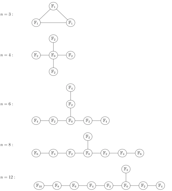
5.1 Non-Higgsable Clusters

Let us begin by cataloguing the phase structure of the non-Higgsable cluster theories. Recall that these are given in F-theory by specific collections of up to three curves, in which the minimal elliptic fibration is always singular. The collection of curves of self-intersection −n

and corresponding 6D gauge algebra are:

Curves 3 4 5 6 7 8 12 3,2 3,2,2 2,3,2

g su(3) so(8) f4 e6 e7 e7 e8 g2×su(2) g2×sp(1) su(2)×so(7)×su(2) (5.1) In the case of the−7 curve theory and multiple curve non-Higgsable clusters, there are also half-hypermultiplet matter fields.

(22)

1

F F

F₁

1

flop C

c

*

shrink

enhance to SU(3)

F₁

A₂ _shrink

*

C' _C'

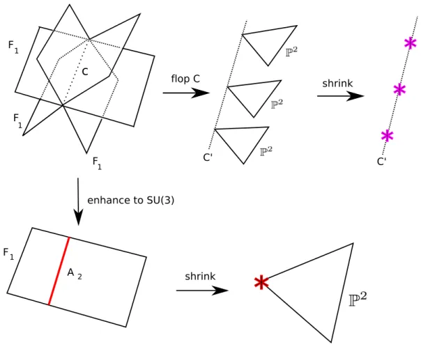
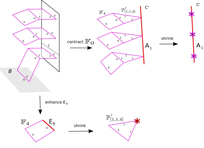
Figure 2: Geometry of the−3 theory. upper left: Reduction of the tensor branch overS1; upper center: flop phase transition; upper right: reduction of the 6D SCFT over S1; lower left: gauge symmetry enhanced toSU(3); lower right: strong coupling limit of

SU(3) theory. In the 5D limit,C0 and _P2 _{decompactify.}

Hirzebruch surfaces. See Appendix A for details.

Let us discuss the physics of this reduction in more detail for one example, the case of the −3 curve. The resulting geometry is depicted in Figure 2. By reducing on the circle the tensor branch of this theory, we obtain a collection of_F1 Hirzebruch surfaces which intersect giving rise to a Kodaira type IV fiber. In Figure 2 we have indicated the curve which we can flop byC. It is a rational curve with anO(−1)⊕ O(−1) normal bundle. Flopping it we obtain a curve C0 with three _P2 surfaces intersecting it at a point. Shrinking these surfaces down to zero size we obtain three 5D SCFTs corresponding to _C3_/

Z3 orbifold points. The remaining curve has the same area as the nearby elliptic curves, so in the limitRS1 →0, the

curve C0 grows to infinite size and the three _C3_/

Z3 theories decouple.

(23)

illustrated in the lower portion of Figure 2. One first shrinks two of the _F1 surfaces to the common curve of intersection, where they form a curve of A2 singularities. To take that gauge theory to strong coupling, we shrink the area of the curve of singularities, leaving a single _P2 _{containing a single conformal point (the strongly coupled}_SU_{(3) theory).}

This example is interesting because it illustrates how, even in a simple situation, non-trivial 5D fixed points can occur in different chambers of the extended K¨ahler cone. The fact that we obtain a 5D SCFT from the phase corresponding to the S1 reduction of the tensor branch has to be regarded as a coincidence, though. The actual reduction of the 6D SCFT onS1 _{is given by the three}

C3/Z3 theories.

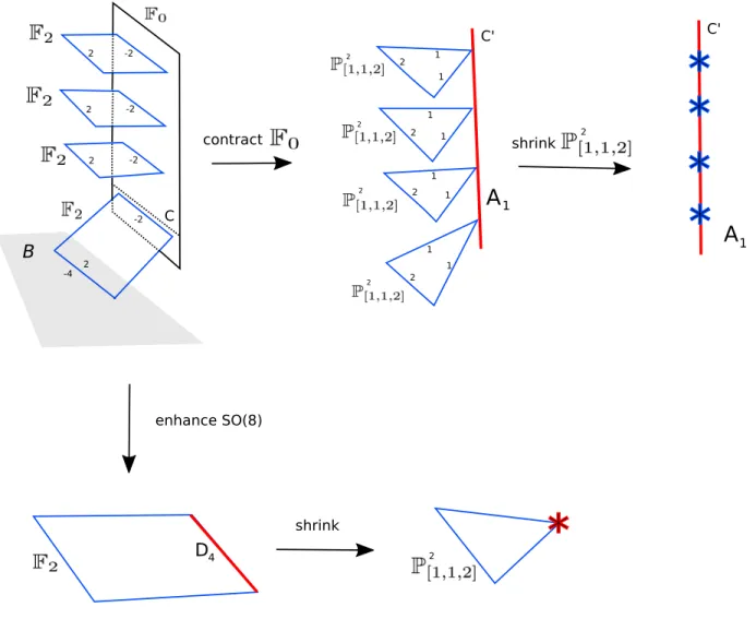
As a second example we consider the case of the −4 curve. The resulting geometry is depicted in Figure 3. By reducing on the circle the tensor branch of this theory, we obtain an F0 Hirzebruch surface meeting fourF2 Hirzebruch surfaces along fibers of one of the rulings of _F0. The intersection pattern gives rise to a Kodaira type I₀∗ fiber. This time, instead of flopping a curve we contract a divisor to a curve, in one of two different ways. If we contract the_F0 along the ruling which includes the intersection curves with the_F2 surfaces, we obtain a curve of SU(2) singularities with four _P2_[1_,₁_,_2] surfaces intersecting it at a point. Shrinking these surfaces down to zero size we obtain four 5D SCFTs corresponding to _C3_/

Z4 orbifold points with group action specified by (1₄,1₄,1₂). The corresponding curve of A1 singularities gives anSU(2) gauge group with gauge couplingg2

SU(2)∼1/vol(C) which is also proportional toRS1. In the limitR_S1 →0, the curve C grows to infinite size and the four_C3/_Z4 theories

decouple. These models have an SU(2) flavor symmetry.

In this case, the S1 reduction of the 6D tensor branch also flows to a fixed point, corre-sponding to the pure SO(8) gauge group without matter. That is illustrated in the lower portion of Figure 3. One first shrinks the _F0 along its other ruling together with three of the _F2 surfaces to a curve ofD4 singularities. To take that gauge theory to strong coupling, we shrink the area of the curve of singularities, leaving a single _P2

[1,1,2] containing a single conformal point (the strongly coupled SO(8) theory).

For the multiple curve theories, however, we do not expect to realize a conformal fixed point in the chamber corresponding to the S1 _{reduction of the moduli space. This again} follows from the criterion put forward in [42], because we always have a product gauge group with bifundamental matter. To reach a conformal fixed point for these geometries, we must perform a flop transition to another chamber of moduli space, namely that described by the orbifold procedure outlined above.

We can carry out the analysis of section 4 for each of these examples quite explicitly. In Table 1, for each p/q corresponding to a non-Higgsable cluster, we describe the finite group action on the variabless,t,x,y and functionsf,g which appear in the corresponding Weierstrass equation, and we also give the lowest order terms in f and g. This data then determines the 5D fixed points after S1 reduction.

(24)

2 -2 2 -2

2 -2

-4

B

contract

A

₁

shrink

2

2 1

1

1 1

*

enhance SO(8)

D₄

shrink

*

2 2

2

A

₁

C

C' C'

Figure 3: Geometry of the −4 theory. upper left: Reduction of the tensor branch over

S1_;

upper center: flop phase transition; upper right: reduction of the 6D SCFT over

S1lower left: gauge symmetry enhanced to SO(8);lower right: strong coupling limit

(25)

p/q (s, t, x, y;f, g) f g

2 (1₂,1₂,0,0; 0,0) f0 g0 3 (1₃,1₃,1₃,0;2₃,0) f0s2+f1st+f2t2 g0 4 (1

4, 1 4,0,

1

2; 0,0) f0 g0

5 (1₅,1₅,4₅,1₅;3₅,2₅) f0s3+f1s2t+f2st2+f3t3 g0s2 +g1st+g2t2 6 (1

6, 1 6,

2 3,0;

1

3,0) f0s 2₊_f

1st+f2s2 g0 7 (1₇,1₇,4₇,6₇;1₇,5₇) f0s+f1t

P5

j=0gjs5−jtj

8 (1 8, 1 8, 1 2, 3 4; 0,

1

2) f0

P4

j=0gjs 4−j_tj

12 (₁₂1 ,₁₂1 ,1₃,1₂;2₃,0) f0 =

P8

j=0fjs8−jtj g0 5/2 (1

5, 2 5, 1 5, 4 5; 2 5, 3

5) f0s

2₊_f

1t g0s3 +g1st+g2t4 7/3 (1₇,3₇,1₇,5₇;2₇,3₇) f0s2+f2t3 g0s3+g1t 8/5 (1

8, 5 8, 1 2, 1 4; 0,

1

2) f0 g0s

4₊_g

1s2t2+g2t4 Table 1: Weierstrass coefficients. All fj and gj are ΓU(2)-invariant functions.

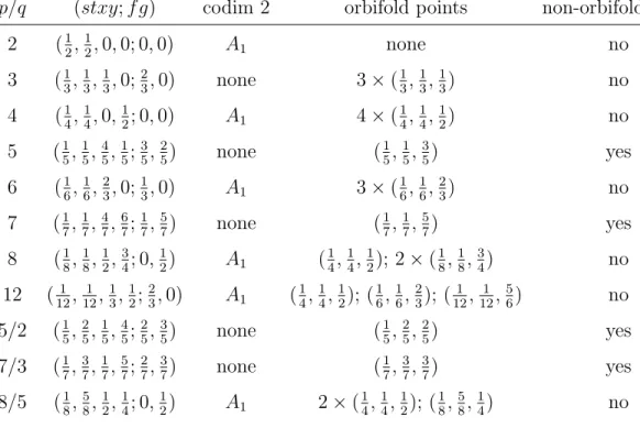
set of the group action, and what subgroup stabilizes each fixed point. This information is tabulated in Table 2. The origin is always fixed by the entire group, but if g0 is constant, the hypersurface does not pass through the origin; in that case, we have written “no” in the non-orbifold column. The orbifold points are specified by their group actions.

5.2 Rigid A-type Theories

Consider next the Rigid A-type theories of reference [7]. These are defined by considering a base B with collapsing curves intersecting as:

n1, ..., nk. (5.2)

We then perform the minimal resolutions necessary to place all elliptic fibers in Kodaira-Tate form. We denote the Hirzebruch-Jung continued fraction by p/q. These theories have no continuous flavor symmetries in six dimensions. Consequently, any flavor symmetries obtained upon reduction to five dimensions should be viewed as emergent in the infrared.

There are at least two disconnected components to the 5D SCFT, and there may be three or four. To determine which case occurs, we follow the analysis in section 4 and see that it is determined by the knowledge of which power of the determinant vanishes.

(26)

p/q (stxy;f g) codim 2 orbifold points non-orbifold point 2 (1₂,1₂,0,0; 0,0) A1 none no

3 (1₃,1₃,1₃,0;2₃,0) none 3×(1₃,1₃,1₃) no 4 (1

4, 1 4,0,

1

2; 0,0) A1 4×( 1 4,

1 4,

1

2) no

5 (1₅,1₅,4₅,1₅;3₅,2₅) none (1₅,1₅,3₅) yes 6 (1

6, 1 6,

2 3,0;

1

3,0) A1 3×(

1 6,

2

3) no

7 (1₇,1₇,4₇,6₇;1₇,5₇) none (1₇,1₇,5₇) yes 8 (1

8, 1 8, 1 2, 3 4; 0,

1

2) A1 (

1 4,

1

2); 2×( 1 8,

1 8,

3

4) no

12 (₁₂1,₁₂1 ,1₃,₂1;2₃,0) A1 (1₄,1₄,1₂); (1₆,1₆,₃2); (₁₂1,₁₂1,5₆) no 5/2 (1

5, 2 5, 1 5, 4 5; 2 5, 3

5) none (

1 5,

2 5,

2

5) yes

7/3 (1₇,3₇,1₇,5₇;₇2,3₇) none (₇1,3₇,3₇) yes 8/5 (1

8, 5 8, 1 2, 1 4; 0,

1

2) A1 2×(

1 4,

1 2); (

1 8,

5 8,

1

4) no

Table 2: Singularity loci.

The cases of interest here appear in block diagonals of the tables in that paper, and in particular, the analysis there shows that there are infinite families of examples for each of the cases analyzed in section 4. That is, there are infinite families of examples with four orbifold points, or with three orbifold points of the same type, and so on. What changes is the codimension 2 singular locus, which can give a (flavor) symmetry of arbitrarily large rank.

For example, p/q = 4N/(2N −1) corresponds to the data

(s, t, x, y;f, g) =

1 4N,

2N −1 4N ,0,

1 2; 0,0

(5.3)

and there are four orbifold points of type (₄1_N,2N₄_N−1,1₂) with a codimension two locus sup-porting an A2N−1 singularity. When the base is fully resolved, it corresponds to 4141· · ·14.

5.3 M5-Brane Probe Theories

(27)

5.3.1 Probes of an ADE Singularity

Consider first the case of M5-branes probing an ADE singularity. The F-theory realization of these 6D SCFTs is straightforward to realize in terms of a pair of colliding singularities, each associated with an algebra of typegADE which intersect at the singular point of the geometry

C2/Zk. Minimal resolution of the orbifold in the base yields a chain of −2 curves, and the

presence of the colliding singularities gives an additional enhancement in the singularity type over each −2 curve. The partial tensor branch is then given by:

[g]2g, ...,2[g]g . (5.4)

In the M5-brane picture, this corresponds to seperating the branes along the _R⊥ factor

of _R⊥×C2/ΓADE. Further blowups between each such collision are required to place all

elliptic fibers in Kodaira-Tate form. Returning to the partial tensor branch of line (5.4), we can read off the reduction to five dimensions. It is given by a generalized 5D quiver, with gauge algebras gADE, and 5D conformal matter. This 5D conformal matter is the CFT

associated with compactification of 6D conformal matter and as such, the analysis of section 4 guarantees that we will indeed reach a fixed point. On the Coulomb branch, this system is, after taking an appropriate flop transition described by the affine quiver gauge theory obtained from D4-branes probing an ADE singularity. Indeed, we note that when we have more than one gauge group factor, the argument of [42] applies, and we do not expect a 5D fixed point in the chamber of moduli space where the quiver gauge theory description is valid. If we go to the full 6D tensor branch and then reduce, we encounter a similar issue.

To reach a 5D fixed point, we would need to perform a sequence of flop transitions, and one region of moduli space where we are guaranteed to find such a fixed point is in circle reduction of the 6D fixed point. Indeed, the F-theory model for this case is also straightforward to engineer. To see why, consider first the model for a single component of the discriminant locus of typegADE. We can parameterize this in terms of the local equation:

y2 =x3+f(s)x+g(s), (5.5) for a single holomorphic coordinate s of _C. In all but the In fiber case, the leading order

behavior of this singularity takes the form:

y2 =x3+sax+sb, (5.6) for some suitable choice ofaandb. To realize a collision in_C2, we then have (see e.g. [9,10]):

y2 =x3+ (st)ax+ (st)b. (5.7)

(28)

choice of gauge algebra) remain the same for this model.

Note also that in this case, the “patch at infinity” withy = 1 does not actually contribute a 5D SCFT. The reason is that the orbifold locus is locally given by _C×_C2_/_Γ

ADE, and so

there are no collapsing divisors in this region of the geometry. Instead, all of the collapsing divisors are concentrated in the patch described by line (5.7).

As a concrete example, we see that the form of colliding E8 singularities, namely a collision of two type II∗ fibers, is:

y2 =x3+ (st)4x+ (st)5. (5.8) We produce a 5D generalized quiver with E8 gauge group factors and (E8, E8) conformal matter by performing a _Zk quotient on the base. Though it would be interesting to perform

a similar analysis of the fully resolved geometry (akin to what we did for the non-Higgsable cluster theories) and to then collapse divisors to reach a canonical singularity, this will of course be much more involved due to the large number of additional compact cycles in this case. We leave this interesting issue for future work.

5.3.2 Probes of an E8 Wall

Consider next the case of M5-branes next to an E8 nine-brane. The F-theory model has a base:

[E8]1,2, ...,2

| {z }

k

, (5.9)

where the E8 flavor symmetry is only manifest in the limit where all curves collapse to zero size. The associated Weierstrass model is:

y2 =x3 +gk(s)t5, (5.10)

where gk(s) is a degree k polynomial in s.

The dimensional reduction of this model to five dimensions has already been determined in the literature. It is given by an Sp(k) gauge theory with N = 7 hypermultiplets in the fundamental representation. In the limit where the gauge theory passes to strong coupling, the flavor symmetry enhances from SO(14) to E8.

(29)

We can also consider a non-trivial fiber enhancement over the curves of line (5.9). This is interpreted as small instantons probing an ADE singularity [85, 9, 12]. In this case, the partial tensor branch is not expected to realize a 5D SCFT upon circle reduction. We can, however, again take a flopped phase of the geometry, i.e., keep all curves of the base at small size when we pass to five dimensions. In this case, we again expect to realize a 5D SCFT.

6 Conclusions

The classification of 6D SCFTs via F-theory provides a starting point for the construction and study of lower-dimensional SCFTs. In this paper we have applied these general consid-erations in the study of 5D SCFTs. Starting from 6D SCFTs realized via F-theory on an elliptically fibered Calabi–Yau threefold, we have shown how further reduction on a circle leads to a rich phase structure for 5D theories, as realized by M-theory compactified on the same Calabi–Yau. In particular, we have seen that the reduction of a 6D N = (1,0) SCFT to five dimensions yields a 5D SCFT, and moreover, the reduction of the tensor branch de-formation of a 6D SCFT typically does not yield a 5D SCFT. In the Calabi–Yau geometry, the two phases are connected by a sequence of flop transitions, namely a trajectory in the extended K¨ahler cone. The existence of these two phases provides a concrete way to pass from one phase to the other, namely, by a flow through moduli space. By elucidating the structure of the 5D conformal fixed points, we have shown in particular how 5D quiver gauge theories can be connected to a class of geometrically realized fixed points. In the remainder of this section we discuss some avenues of future investigation.

One of the important uses of a 5D gauge theory analysis is the potential to explicitly compute the structure of an associated supersymmetric index. Now, even though we have argued that one must flop to another chamber of moduli space to actually realize the fixed point, the sense in which this object transforms under flops should be well controlled. In this sense, gauge theory methods for calculating such quantities should have an interpretation in terms of a superconformal index. This is indeed the philosophy adopted in much of the literature on 5D SCFTs (see e.g. [45,86,87]), though with the explicit geometry now in hand, one can in principle check these claims by direct calculation of topological string amplitudes on the Calabi–Yau in the conformal chamber, perhaps along the lines of [17].

Now that we have constructed a broad class of new 5D SCFTs, it is natural to ask whether some of these also yield holographic duals, perhaps along the lines of [46, 88, 50, 51]. Circle reduction ofAdS7 vacua does not yieldAdS6 vacua, which is in accord with the phase structure observed in this work. We have also seen, however, that flop transitions often yield a 5D fixed point. It would be interesting to understand this holographically.

(30)

interesting to determine whether some generalization of the numerical invariants used in the classification of 6D SCFTs can be obtained for this class of geometries as well. Let us note that from a physical perspective, one might be tempted to conjecture that all 5D SCFTs are obtained from some deformation of a 6D SCFT on a circle. This looks difficult to arrange in all cases, since, for example, supersymmetric orbifolds of the form _C3/ΓSU(3) for ΓSU(3) a finite subgroup ofSU(3) do not have a clear embedding in an elliptically fibered Calabi–Yau threefold of the sort used to engineer 6D SCFTs via F-theory. Either establishing a firm counterexample, or developing a clear method of embedding 5D SCFTs in 6D theories would be most instructive.