B
OOTSTRAPPINGMAX
TESTS IN THE
PRESENCE OF
W
EAKIDENTIFICATION
John W. Dennis, III
A dissertation submitted to the faculty of the University of North Carolina at Chapel Hill in par-tial fulfillment of the requirements for the degree of Doctor of Philosophy in the Department of
Economics.
Chapel Hill 2019
c
2019
ABSTRACT
JOHN W. DENNIS, III: Bootstrapping Max Tests in the Presence of Weak Identification. (Under the direction of Jonathan B. Hill)
ACKNOWLEDGMENTS
TABLE OF CONTENTS
LIST OF TABLES . . . ix
LIST OF FIGURES . . . x
1 INTRODUCTION AND RELATIONSHIP WITH THE LITERATURE . . . 1
2 TESTING WHITE NOISE WHEN SOME PARAMETERS MAY BE WEAKLY IDENTIFIED . . . 7
2.1 Introduction . . . 7
2.2 Preliminary Notation and Assumptions . . . 15
2.3 Assumptions and Main Results . . . 20
2.3.1 Assumptions . . . 20
2.3.2 Main Results . . . 24
2.3.3 Critical Values . . . 28
2.4 Bootstrap Critical Value Computation . . . 30
2.4.1 Bootstrap Algorithm . . . 31
2.5 Simulations . . . 35
2.5.1 Simulation Results: STAR(1) Model . . . 39
2.5.2 Simulation Results: ARMA(1,1) Model . . . 43
2.6 Empirical Analysis . . . 45
2.7 Conclusion . . . 49
3 TESTING MANY ZERO RESTRICTIONS UNDER MIXED IDENTIFICATION STRENGTH . . . 51
3.2 Relationship with the Literature . . . 53
3.3 The Max Test . . . 58
3.3.1 Parsimonious Models . . . 60
3.3.2 Max Test Framework . . . 61
3.3.3 Empirical Example . . . 64
3.4 Assumptions and Preliminary Results . . . 65
3.4.1 Limit Theory for Parsimonious Estimators . . . 65
3.4.2 Linking the Unrestricted and Parsimonious Models . . . 78
3.5 Max Test Limit Theory and Inference . . . 81
3.5.1 Inference . . . 83
3.5.2 Conditional Simulation Based Inference . . . 84
3.5.3 Residual Multiplier Bootstrap . . . 85
3.5.4 Robust Inference . . . 86
3.6 Additional Examples . . . 87
3.6.1 Testing for Nonlinearity in Exchange Rate Dynamics . . . 88
3.6.2 Weak Identification in Time Series . . . 90
3.6.3 Nonlinear Binary Choice Model . . . 92
3.6.4 Linear IV Model . . . 93
3.7 Monte Carlo Simulations . . . 97
3.8 Conclusion . . . 103
A APPENDIX FOR TESTING WHITE NOISE WHEN SOME PARAMETERS MAY BE WEAKLY IDENTIFIED . . . 105
A.1 Appendix: Proofs of Main Results . . . 105
A.1.1 Appendix: Proof of Lemma 2.3.1 . . . 105
A.1.2 Appendix: Lemma A.1.2 . . . 108
A.2 Appendix: Supporting Lemmas and Proofs . . . 142
A.2.1 Lemmas and Proofs relating to ULLNs formt . . . 142
A.2.2 Lemmas and Proofs relating to the covariance expansion . . . 146
B APPENDIX FOR TESTING MANY ZERO RESTRICTIONS UNDER MIXED IDENTIFICATION STRENGTH . . . 153
B.1 Appendix: Notation . . . 153
B.1.1 Drifting Sequences . . . 154
B.1.2 Grouping Notation . . . 155
B.1.3 Concentrated Criterion Functions . . . 156
B.2 Appendix: Limit Theory for Models with Mixed Identification Strength . . . 157
B.3 Appendix: Supporting Lemmas and Proofs for the Estimator Limit Theory . . . 169
B.4 Appendix: Proofs for the Parsimonious Estimator Limit Theory . . . 173
B.4.1 Appendix: Pointwise Parsimonious Estimator Limit Theory . . . 173
B.4.2 Appendix: Proofs for the Joint Parsimonious Estimator Limit Theory . . . 175
B.5 Appendix: Proofs for the Max Test . . . 177
B.6 Appendix: Additional Proofs . . . 181
LIST OF TABLES
1.1 Identification Categories: Andrews and Cheng’s (2012a) Table I . . . 3
2.1 White Noise Test, No Expansion . . . 40
2.2 White Noise Test, Least Favorable Critical Values . . . 40
2.3 White Noise Test, Size Shrinkage . . . 41
2.4 White Noise Test, Strong Identification, STAR model . . . 42
2.5 White Noise Test, Weak Identification, STAR model . . . 43
2.6 White Noise Test, Strong Identification, ARMA model . . . 45
2.7 White Noise Test, Weak Identification, ARMA model . . . 45
2.8 White Noise Test Empirical Exercise . . . 48
3.1 Max Test Initial Simulations . . . 62
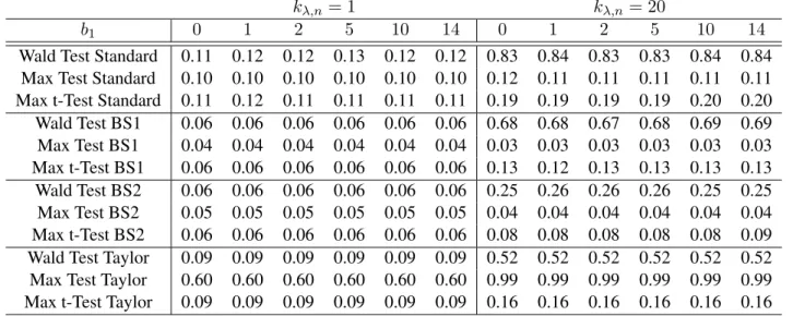
3.2 Max Test Simulations, Null Hypothesis . . . 100
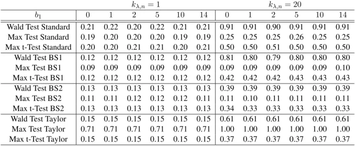
3.3 Max Test Simulations, Local Alternative Hypothesis . . . 102
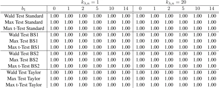
3.4 Max Test Simulations, Alternative Hypothesis . . . 103
LIST OF FIGURES
3.1 Empirical Distribution of the Max Test,kλ = 1 . . . 101
CHAPTER 1
INTRODUCTION AND RELATIONSHIP WITH THE LITERATURE
I describe the use of max tests in the presence of weak identification. This collection informs the reader of some issues that can arise in common inferential analyses in Economics due to the presence of weak identification in the parameters and presents solutions to these problems within the framework of a convenient testing procedure. I consider two practical inferential problems, and for each I discuss how the presence of weak identification can lead to distorted inference and present a method to conduct inference in an appropriate manner.
The two classes of inferential problems I consider are white noise tests and tests on a large dimensional parameter. White noise tests fall within the class of model diagnostic tests; they are designed to aid the practitioner in determining if a particular model is able to capture all of the serial correlation present in the data. In this sense, they can be thought of as one of a group of tests that examines the adequacy of the model in describing the data. In the first paper, I present a white noise test that is appropriate for residuals from estimated models and is robust to parameter identification failure in the model.
The second class of tests has become a focus in the literature in recent years due to the vast quantities of data that have become available to researchers. In particular, researchers often have many variables in a dataset leading to many objects that must be estimated and tested. In the second paper, I present a test for many zero restrictions in a model with a large dimensional parameter when many of the parameter elements may be only weakly identified.
consider in the relevant chapters below.
Identification failure is present in both problems that I consider, but here I must be specific regarding the meaning of identification failure. Lewbel (ming) indicates the term identification failure appears in more than two dozen forms in the literature, but all share a common underlying meaning. In particular, an object is not identified if its true value cannot be uniquely determined in the population. I specifically use utilize the definition of Andrews and Cheng (2012a) to describe identification failure as the situation in which there is a known parametric source of identification failure for a parameter in the model under consideration. The framework of Andrews and Cheng (2012a) is convenient for the econometrician in describing parametric identification failure, as it allows a range of identification behaviors to exist between identification and non-identification.
Consider estimating scalar parameters(β, π)from the nonlinear functionYt =βg(Xt, π) +εt
for some smooth non-linear function g. It is well known that when β 6= 0, π can be (strongly) identified, and when β = 0, π cannot be identified. In order to develop a unifying testing frame-work, we utilize a thought experiment which can be characterized by using the notion of drifting sequences of true parameters. Letβ =βnbe a sequence of true parameters, indexed by the sample
sizen, that are drifting to 0. Then the strength of identification ofπ is categorized by the speed at which βn → 0. When
√
nβn → ∞, we characterize π as being semi-strongly identified, and
when√nβn → b ∈ (0,∞), we say πis weakly identified. In the latter case, our estimatorπˆn is
not consistent for the trueπ0, and converges instead to a random variable under certain conditions.
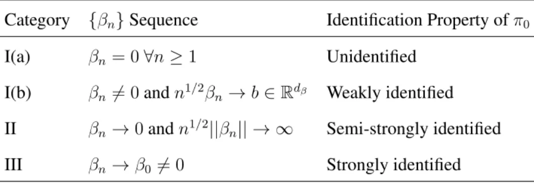
Table 1 from Andrews and Cheng (2012a) details these categories. It is important to note that in this literature, the parametric source of identification failure is known. More recently, Han and McCloskey (2016) develop theory for the case in which the source of identification failure may be unknown. We focus on the former case and leave this extension for future research.
For the cases of non-identification and weak identification, the estimators forπare inconsistent. Further, in these cases the estimator for β is consistent; however, it is a function of πˆn which
converges to a random variable, resulting in a non-standard distribution forβˆn. This implies that
Table 1.1: Identification Categories: Andrews and Cheng’s (2012a) Table I
Category {βn}Sequence Identification Property ofπ0
I(a) βn= 0∀n≥1 Unidentified
I(b) βn6= 0andn1/2βn→b∈Rdβ Weakly identified
II βn→0andn1/2||βn|| → ∞ Semi-strongly identified
III βn→β0 6= 0 Strongly identified
This poses problems for tests based on residuals from model estimation. Non-standard behavior of the estimators propagates through to the test statistic, yielding a non-standard distribution for the test statistic and resulting in potentially distorted inference from traditional tests.
Further, this is an issue for economic practitioners, as many commonly used models in Eco-nomics include parameters that may be unidentified in certain parts of the parameter space. Exam-ples such as Dynamic Stochastic General Equilibrium models (Guerron-Quintana, Inoue, and Kil-ian, 2013; Andrews and Mikusheva, 2015), Smooth Transition AutoRegressive models (Terasvirta, 1994; Ter¨asvirta, 1998; van Dijk, Ter¨asvirta, and Franses, 2002; Andrews and Cheng, 2013), Pro-bit models (Andrews and Cheng, 2012a, 2014) and Nonlinear Binary Choice Models (Andrews and Cheng, 2013), nonlinear instrumental variables models with possibly weak instruments (An-drews and Cheng, 2012a, 2014), ARMA models An(An-drews and Ploberger (1996); An(An-drews and Cheng (2012a); Dennis (2019), Regime Switching Models (Chen, Fan, and Liu, 2016) and Fuzzy Regression Discontinuity Designs (Feir, Lemieux, and Marmer, 2016), models based on moment conditions and GMM (Andrews and Cheng, 2014), and MiDAS Regressions (Ghysels, Hill, and Motegi, 2016b) have been shown to include model components that may not be identified in certain regions of the parameter space.
H0 :β = 0. Under this null hypothesis, theπjare unidentified nuisance parameters, so this
frame-work is related to the literature on testing with nuisance parameters under the null (Davies, 1977, 1987; Andrews and Ploberger, 1994; Hansen, 1996; Stinchcombe and White, 1998; Ghysels and Guay, 2004; Andrews and Mikusheva, 2016). Nuisance parameters cause the test statistics to have non-standard distributions, which often do not have analytic expressions and must be simulated.
In this framework, however, each parameter πj may exhibit its own degree of identification
strength, so a uniformly valid test becomes necessary. Andrews and Cheng (2012a, 2013, 2014) discuss uniformly valid inference but do not allow for mixed identification strength. Cheng (2015) offers the first uniformly valid inference procedure for inference on sub-vectors ofβ allowing for mixed identification strength but limits her theory to additive nonlinear models.
Andrews and Cheng (2012a, 2013, 2014) and Cheng (2015) discuss inference under weak iden-tification but do not consider large dimensional parameters or max test statistics, implementation of a bootstrap, or tests on objects from estimated models, such as white noise tests, that are not tests directly on the model parameters. In contrast, in the first paper, we consider white noise tests based on the maximum of a sequence of correlations that we implement with a bootstrap, and in the second paper, we construct a test based on the maximum of a sequence of estimated parameters from a high dimensional parameter.
The testing procedures that I consider in both classes of problems are based on max tests. When testing the maximum value in a sequence, we are often interested in determining if any of the parameter elements are different from zero. In considering only the maximum from the sequence of values, the max test statistic utilizes the most informative measure available from our data, eliminating issues that arise from low degrees of freedom and inversion of large or near singular covariance matrices when a large number of variables needs to be tested (Hill and Dennis, 2018; Ghysels, Hill, and Motegi, 2016a), or by combining noisy estimates, which occurs when calculating serial correlations at long lags (Hill and Motegi, 2018).
literature1 dating at least to Fisher and Tippet (1928) and Gnedenko (1943). See also Gumbel
(1958) and Berman (1964). Typically in this literature, extreme value theory arguments appeal to the Extremal Types Theorem to determine the exact asymptotic distribution of the maximum statistic (de Haan, 1976). For example, Xiao and Wu (2014) provide a test for serial correlation for observed sequences using the maximum sample autocovariance and show that under suitable normalization, the test statistic converges in distribution to a Gumbel (type I extreme value) dis-tribution. These arguments require that when the data are divided into blocks, the dependence between increasingly distant blocks decays at a sufficient rate as with a mixing condition.
Hill and Motegi (2018); Hill and Dennis (2018) argue that when estimating parsimonious mod-els, allowing for general dependence in the data generating process, or residuals to be used in the max statistic, the classical extreme value theory arguments are no longer straight forward to prove and may require more stringent assumptions than are needed by other methods. Further, extreme value theoretic arguments for establishing the limiting distribution of the maximum of a sequence of values often relies on Gaussianity of the underlying sequence. Hill and Motegi (2018); Hill and Dennis (2018) develop theory that does not rely on Gaussianity and that allows the use of the dependent wild bootstrap (Shao, 2010, 2011a) to mimic the finite sample distribution of the max statistic.
For these reasons, I simulate the distribution of the test statistics with forms of a Wild, or Gaussian multiplier, bootstrap (Wu, 1986; Liu, 1988). Methods for bootstrapping high dimensional statistics have not been available until recently. Chernozhukov, Chetverikov, and Kato (2013, 2017) develop a theory that is able to both bypass the typical extreme value theoretic asymptotic arguments and deliver an impressive growth rate for the sequence being examined.2 However, they
require independence, and their theory is only appropriate for observed random variables and relies on Gaussian approximation that is not appropriate for approximations of non-Gaussian normalized summands. Zhang and Cheng (2018) extend the Gaussian approximation theory in Chernozhukov
et al. (2013, 2017) to allow for dependence, but only allow for observed random variables. Zhang and Wu (2017) develop theory for a Gaussian approximation for high dimensional times series but only allow for observed sequences as well. The theory in Hill and Dennis (2018); Hill and Motegi (2018) is also able to bypass extreme value theoretic arguments, allows for dependence under the null, and is appropriate for residuals. For this reason, we rely on the theory developed in Hill and Motegi (2018); Hill and Dennis (2018).
CHAPTER 2
TESTING WHITE NOISE WHEN SOME PARAMETERS MAY BE WEAKLY IDENTIFIED
2.1 Introduction
We develop a bootstrapped white noise test for residuals that is based on the maximum cor-relation and is robust to parameter identification failure in the model. It is well known that the asymptotic and finite sample distributions of estimators are non-standard when the model contains parameters that are weakly identified, and that standard inference based on t orχ2distributions can
be distorted. For example, Andrews and Cheng (2012a) demonstrate in their figures 1 and 2 that densities of the estimators from an ARMA(1,1) model can be quite different from normal when the AR and MA parameters are close to the same value. Further, Cheng (2015) shows in her table 1 that using standard normal critical values for tests on a parameter from an additive nonlinear model with a weakly identified parameter can generate large size distortions.
The impact of identification failure on the distributions of the estimators for a model can prop-agate beyond tests on the parameter values. When the test statistic is based on an estimated model, the usual method to either prove the asymptotic distribution of the test statistic or to implement a finite sample correction via a bootstrap is to utilize a first order expansion of the test statistic that involves the distribution of the parameter estimators. This enables inference on the test statistic to properly account for the impact of model estimation.
In particular, this is an issue for economic practitioners engaging in model diagnostic activi-ties, as many commonly used models in Economics include parameters that may be unidentified in certain parts of the parameter space. Examples such as Smooth Transition AutoRegressive models (Terasvirta, 1994; van Dijk et al., 2002; Andrews and Cheng, 2013), Probit models (Andrews and Cheng, 2012a, 2014) and Nonlinear Binary Choice Models (Andrews and Cheng, 2013), nonlinear instrumental variables models with possibly weak instruments (Andrews and Cheng, 2012a, 2014), ARMA models (Andrews and Ploberger, 1996; Andrews and Cheng, 2012a), Regime Switch-ing Models (Chen et al., 2016) and Fuzzy Regression Discontinuity Designs (Feir et al., 2016), Dynamic Stochastic General Equilibrium models (Guerron-Quintana et al., 2013; Andrews and Mikusheva, 2015), models based on moment conditions and GMM (Andrews and Cheng, 2014), and MiDAS Regressions (Ghysels et al., 2016b) have been shown to include model components that may not be identified in certain regions of the parameter space. The models above are often used under the assumption of a white noise error term. The current paper focuses on testing if the error term is a white noise process while allowing for some model parameters to be unidentified in parts of the support of the parameter space. The test presented in this paper, then, can be viewed as a test of model adequacy for models such as those mentioned above, which may have identification failure in regions of the parameter space.
There are three key components that characterize this test. First, this test is a white noise corre-lation test for residuals that only requires uncorrelatedness under the null. Allowing for residuals requires that we account for the influence of the estimated parameters on our test statistic. In par-ticular, we allow for models in which some parameters may be non- or weakly identified in the sense of Andrews and Cheng (2012a), leading to inconsistent estimators. Utilizing a first order expansion of our test statistic about the point of identification failure allows us to account for the influence of the estimated parameters without the need for a consistent estimator for the parameters that are not identified.
a traditional portmanteau test which utilizes the sum of all squared sample correlations, the max-imum statistic only focuses on the most informative sample correlation and, therefore, mitigates both the issue of washing out a single non-zero correlation in an average when testing for potential correlations at many lags and issues stemming from noisy sample correlation estimates that can occur at long lags. Further, max statistics are convenient for high dimensional objects, as they do not require inversion of a large covariance matrix.
Traditional arguments for statistics of a maximum value rely on proving asymptotic conver-gence via the extremal types theorem (de Haan, 1976), but these arguments are typically for ob-served sequences, and bootstraps are not typically considered for finite sample improvement. Xiao and Wu (2014) discuss a similar maximum statistic and prove that under suitable normalizing con-stants their test statistic converges to a type I extreme value distribution; however, they do not allow for residuals, an important distinction that affects the extreme value theory asymptotic argument, and they do not prove the validity of their bootstrap. Further, the extreme value theory approach re-quires restrictions to ensure convergence that are not necessary under our bootstrapping approach. We bypass standard extreme value theory arguments by use of theory in Hill and Dennis (2018) and Hill and Motegi (2018) paired with the dependent wild bootstrap of Shao (2010, 2011a).
unidentified parameters. We construct our identification robust test by bootstrapping the test statis-tic under both scenarios and stitching the resulting cristatis-tical values together with an identification pre-test as discussed in Andrews and Cheng (2012a).
Throughout the paper, we assume a general model for the residuals from a regression model, which we denote εt(θ), where θ are the parameters of the model. For clarity, we elaborate the
details for our test with an ARMA model (e.g.Yt=βYt−1+εt−πεt−1) and an additive nonlinear
model, an example of which is the Smooth Transition Autoregressive model of Terasvirta (1994): Yt =βXt×g(Zt, π) +ζXt+εt,whereXttypically contains lags ofYt,g is a smooth, nonlinear
function1 and εt is the model error, which we estimate with the regression residualsεt(ˆθn). Our
goal is to test if{εt}is a white noise process:
H0 :ρ(h) = 0∀h∈N vs. HA:ρ(h)6= 0 for someh∈N
whereρ(h) =E(εtεt−h)/E(εtεt). To test this hypothesis, we specifically consider the sample max
correlation statistic (Hill and Motegi, 2018)
ˆ
Tn= √
n max
1≤h≤Ln
|ρˆn(h)|,
where{Ln}is a sequence of integers with Ln → ∞as n → ∞, Ln = o(n) allowing for a true white noise test.2 We utilize the dependent wild bootstrap (Shao, 2010, 2011a) paired with an expansion of our test statistic to account for the dependence upon the estimated parameters. This allows our test to be appropriate for residuals as in Hill and Motegi (2018); however, the test in Hill and Motegi (2018) requires consistency of all parameter estimators and, thus, cannot accom-modate models in which some parameters are weakly identified. Our test is designed specifically to accommodate such models.
1common examples are the logistic and exponential functionsg(z, π) = (1−exp{−π
1(z−π2)})−1andg(z, π) = 1−exp{−π1(z−π2)2}forπ1>0. See e.g. van Dijk et al. (2002).
Our white noise test, however, is robust to parameter identification failure. Consider estimating scalar parameters (β, π) from the nonlinear model Yt = β0g(Zt, π0) + εt for some non-linear
functiong. It is well-known thatπ0 can be (strongly) identified whenβ0 6= 0, and whenβ0 = 0, π0 cannot be identified. In order to accommodate non-identification, we adopt the identification
unifying framework of Andrews and Cheng (2012a). This framework is characterized by the notion of drifting sequences of true parameters. Let β ≡ βn be a sequence of true parameters that are
drifting to 0, the point of identification failure for this example. Andrews and Cheng (2012a) categorize the strength of identification ofπ0 by the speed at which βn → 0. If βn → 0 slowly
enough, then one can still consistently estimateπ0, and we say thatπ0 is semi-strongly identified.
However, ifβn → 0too quickly, then one cannot consistently estimate π0, and we say thatπ0 is
weakly identified. Table 1 from Andrews and Cheng (2012a) details the rates associated with these categories. It is important to note that in this literature the source of identification failure is known; that is, our model tells us specifically thatβ = 0 results in identification failure. More recently, Han and McCloskey (2016) develop theory for the case in which the source of identification failure is unknown. We focus on the former case and leave this extension for future research.
Note that the estimator for βis consistent, regardless of the identification strength ofπ. How-ever, the estimator for β is a function of the estimator for π, βˆn ≡ βˆn(ˆπn), and ˆπn converges
to a random variable when π0 is not consistently estimable, yielding a non-standard distribution
for βˆn.3 This poses problems for tests based on residuals from model estimation. Non-standard
behavior of the estimators propagates through to the test statistic, yielding a non-standard distri-bution for the test statistic and resulting in potentially distorted inference from traditional tests. The limiting distribution of our test statistic can be categorized by whetherπ0 is consistently
es-timable or not, so we group weak identification and non-identification together and refer to them as weak identification, and we collectively refer to strong and semi-strong identification as strong identification.
This paper is related to but different from the literature on hypothesis testing with a nuisance
parameter. Davies (1977, 1987) provide early references for hypothesis tests with nuisance pa-rameters under the null. See also Hansen (1996), Stinchcombe and White (1998), Ghysels and Guay (2004), and more recently Andrews and Mikusheva (2016). Andrews and Ploberger (1994) discuss optimal tests with a nuisance parameter under the null. Andrews and Ploberger (1996) develop a test for white noise against an ARMA(1,1) alternative since these models provide a par-simonious representation of a broad class of stationary time series. As noted by Nankervis and Savin (2010), Poterba and Summers (1988) show that many financial return series can be repre-sented by ARMA(1,1) models. In their model, the ARMA(1,1) reduces to a white noise process under the null, making the MA coefficient a nuisance parameter.
Andrews and Cheng (2012a, 2013, 2014) and Cheng (2015) discuss inference under weak identification but do not consider max test statistics, implementation of a bootstrap, or tests on objects from estimated models, such as white noise tests, that are not tests directly on the model parameters. In contrast, we consider white noise tests based on the maximum of a sequence of correlations that we implement with a bootstrap.
White noise tests have a long history, dating in some form to at least Box and Pierce (1970) and Ljung and Box (1978). In addition to portmanteau tests, spectral tests (Hong, 1996; Shao, 2011a) are also widely considered in the literature. Many early tests for serial correlation are based on i.i.d. Gaussian assumptions and required a finite maximum lag length cutoff. We are specifically interested in true white noise tests, which are able to accommodate asymptotically infinitely many lags, as questions such as the efficient market hypothesis are related to true white noise tests (Hill and Motegi, 2019).
that the asymptotic distribution of the correlation coefficients of residuals from ARMA processes do not follow the standard chi-square distribution when the errors are uncorrelated but dependent, and using chi-square critical values in this situation leads to distorted inference.
Often, the martingale difference sequence errors are modeled using GARCH processes, and standardized residuals are used to construct the sample serial correlation even though these tests do not have standard asymptotic distributions. Chen (2008) provides tests for autocorrelation specif-ically for models with GARCH based errors, but these tests assume that the model is correctly specified. Francq et al. (2005) and Nankervis and Savin (2010, 2012) develop tests that do not rely on a correctly specified model for the conditional variance. Further, Nankervis and Savin (2010, 2012) note that the assumption of martingale difference errors may be too restrictive. As a result, recent interest has focused on uncorrelated dependent time series (Nankervis and Savin, 2010, 2012; Shao, 2011a,b; Zhu and Li, 2015; Zhang, 2016; Hill and Motegi, 2018).
Our test is based on the maximum sample serial correlation, and when testing the maximum value in a sequence, we are most often interested in determining if any of the parameter elements are different from zero. In considering only the maximum from the sequence of values, the max test statistic utilizes the most informative measure available from our data, eliminating issues that arise from low degrees of freedom and inversion of large or near singular covariance matrices when a large number of variables needs to be tested (Hill and Dennis, 2018; Ghysels et al., 2016a), or by combining noisy estimates, which occurs when calculating serial correlations at long lags (Hill and Motegi, 2018).
Statistics based on a maximum of a sequence of values is an extensively studied topic in the literature4 dating at least to Fisher and Tippet (1928) and Gnedenko (1943). See also Gumbel
(1958) and Berman (1964). Typically in this literature, extreme value theory arguments appeal to the Extremal Types Theorem to determine the exact asymptotic distribution of the maximum statistic (de Haan, 1976). For example, Xiao and Wu (2014) provide a test for serial correlation for observed sequences using the maximum sample autocovariance and show that under suitable
normalization, the test statistic converges in distribution to a Gumbel (type I extreme value) dis-tribution. These arguments require that when the data are divided into blocks, the dependence between increasingly distant blocks decays at a sufficient rate as with a mixing condition.
Hill and Motegi (2018) and Hill and Dennis (2018) argue that when allowing for general de-pendence in the data generating process and residuals to be used in the max statistic, the classical extreme value theory arguments are no longer straight forward to prove and may require more stringent assumptions than are needed by other methods. Further, extreme value theoretic argu-ments for establishing the limiting distribution of the maximum of a sequence of values often relies on Gaussianity of the underlying sequence. Hill and Motegi (2018) and Hill and Dennis (2018) develop theory that does not rely on Gaussianity and that allows the use of the dependent wild bootstrap (Shao, 2010, 2011a) to mimic the finite sample distribution of the max statistic.
The bootstrapped white noise test in Hill and Motegi (2018) is based on the maximum se-rial correlation and allows for a weaker moment contraction property than that in Xiao and Wu (2014) and side-steps asymptotic extremal value theory arguments by exploiting convergence of
{√n(ˆγ(h)−γ(h)) : 1 ≤ h ≤ L}to a Gaussian process for each L ∈N paired with arguments dating to Ramsey (1929). This method requires weaker conditions than the extreme value theo-retic approach but results in the trade-off that an upper bound on the sequenceLn → ∞cannot be provided.5 Further, Hill and Motegi (2018) ignore the possibility of nuisance parameters and only allow for strong identification of all parameters in the model estimation step.
Methods for bootstrapping high dimensional statistics have not been available until recently. Chernozhukov et al. (2013, 2017) develop a theory that is able to both bypass the typical extreme value theoretic asymptotic arguments and deliver an impressive growth rate for the sequence being examined. However, they require independence, and their theory is only appropriate for observed random variables and relies on Gaussian approximation that is not appropriate for approximations
5Hill and Motegi (2018) address the issue of optimal lag selection with a data driven procedure, modified from the
of non-Gaussian normalized summands.6 Zhang and Cheng (2018) extend the Gaussian
approx-imation theory in Chernozhukov et al. (2013, 2017) to allow for dependence, but only allow for observed random variables. Zhang and Wu (2017) develop theory for a Gaussian approximation for high dimensional times series but only allow for observed sequences as well. The theory in Hill and Dennis (2018) and Hill and Motegi (2018) is also able to bypass extreme value theoretic arguments, allows for dependence under the null, and is appropriate for residuals. For this reason, we rely on the theory developed in Hill and Motegi (2018) and Hill and Dennis (2018).
For model estimation, we adopt the notation of Andrews and Cheng (2012a). Section 2.2 discusses the preliminary notation and assumptions needed to fit within their framework. Section 2.3 presents the main assumptions and results, and we present the bootstrap and prove its validity in section 2.4. Section 2.5 presents the Monte-Carlo simulations. All proofs and supporting lemmas are collected in the appendix.
2.2 Preliminary Notation and Assumptions
The true parameter isγ = (θ, φ)with compact true parameter space
Γ ={γ = (θ, φ) :θ∈Θ∗, φ∈Φ∗(θ)}
whereθ = (β, ζ, π) = (ψ, π), ψ = (β, ζ), and we assumeψ is always identified andζ does not effect the identification of π, and φ is an additional parameter such that γ = (θ, φ) completely determines the distribution of the data. For someγ ∈Γ, expectation under the true distribution of
{(Yt, Xt, εt)}={Wt :t≤n}is denotedEγ.
Since the estimatorπˆnforπnis inconsistent, we make use of the following concentrated
crite-rion functionQc
n(π)and estimatorψˆn(π). Defineψˆn(π)∈Ψ(π)for a givenπ∈Πby
Qn( ˆψn(π), π) = inf
ψ∈Ψ(π)Qn(ψ, π) +op(n −1)
and defineπˆn∈Πby
Qcn(ˆπn) =Qn( ˆψn(ˆπn),πˆn) = inf
π∈ΠQn( ˆψn(π), π) +op(n −1).
Observe( ˆψn(ˆπn),πˆn) = ˆθn= infθ∈ΘQn(θ) +op(n−1).
We adopt the notation of Andrews and Cheng (2012a) in order to define cases that differentiate weak and (semi-)strong identification. The theory relies on the following drifting sequences of true parameters. Define the set of true drifting sequences asΓ0 ={{γn∈Γ : n≥1}:γn →γ0 ∈ Γ},
and define the drifting cases:
(i) Γ(γ0,0, b) ={{γn} ∈Γ0 :β0 = 0, n1/2βn →b∈(R∪ {±∞})dβ}
(ii) Γ(γ0,∞, ω0) = {{γn} ∈Γ0 :n1/2βn → ∞, βn/||βn|| →ω0, ||ω0||= 1}.
In our model, the identification ofπis based on whether or not the parameterβ = 0. In terms of these drifting sequences, π0 is not identified asymptotically when the limiting parameterβ0 = 0.
Further, in the case thatβ0 = 0, the speed at whichβn → β0 = 0affects the asymptotic analysis.
In particular, whenβn →0fast enough, given by case(i)with||b||<∞, we say the parameterπ0
isweaklyidentified. In this case, the estimatorˆπn is not consistent. Case two gives the definitions
ofsemi-strongidentification, whenβ0 = 0andstrongidentification, whenβ0 6= 0.
In the (semi-)strong identification casesπˆnis consistent, and we employ first order expansions
around the true parameterθn. However, since πˆn is not consistent under weak identification, an
expansion around θn = (ψn, πn) is not appropriate. Inspired by the expansion of the criterion
function about the point of non-identification in Andrews and Cheng (2012a), we expand our test statistic about the point of non-identification in the weak identification case in order to deal with the inconsistency ofπˆn. Recall the point of non-identification isβ0 = 0. Defineψ0,n = (0, ζn)and
Q0,n =Qn(ψ0,n, π).
Define
ξ(π;γ0, b) = −
1
2(G(π) +K(π, π0)b) 0
whereG is a mean zero Gaussian process,H is a Hessian, and K arises as a bias correction. Assumeπ∗(γ0, b) = argmin
π∈Π
ξ(π;γ0, b).
More specifically, under {γn} ∈ Γ(γ0,0, b) with||b|| < ∞, the mean zero Gaussian process
{G(π;γ0) :π ∈Π}is defined as the limit of the process{Gn(π;γ0) :π∈Π}defined by
Gn(ψ0,n, π) = n1/2 (
∂
∂ψQn(ψ0,n, π)−Eγn ∂
∂ψQn(ψ0,n, π)
)
=n−1/2
n X
t=1
mψ(Wt, ψ0,n, π)−Eγnmψ(Wt, ψ0,n, π)
where ∂ψ∂ Qn(θ) =n−1
Pn
i=1mψ(Wt, θ). H(π;γ0)is the nonstochastic symmetricdψ×dψ matrix
valued function, continuous onΠthat is the uniform (inπ) limit ofHn(ψ, π;γ0) = ∂ψ∂ ∂ψ∂0Qn(ψ, π).
Finally,Kn(θ;γ0) =n−1
Pn
t=1
∂
∂β0Eγ0m
ψ(W t, θ).
Assumption 1(Weak Identification Objects). Under{γn} ∈Γ(γ0,0, b)with||b||<∞,
(i) Gn(·) ⇒ G(·;γ0), where G(·;γ0) is a mean zero Gaussian process indexed byπ ∈ Π with bounded continuous sample paths and a.s. p.d. covariance kernel
Ω(π,π˜;γ0)≡E[G(π;γ0)G(˜π;γ0)0]forπ,π˜∈Π.
(ii) supπ∈Π||Hn(ψ0,n, π)−H(π;γ0)||
p −
→ 0for some nonstochastic symmetricdψ ×dψ
matrix-valued function H(π;γ0) on Π × Γ that is continuous on Π for all γ0 ∈ Γ and λmin(H(π;γ0))>0andλmin(H(π;γ0))<∞ ∀π ∈Πfor allγ0 ∈Γwithβ0 = 0.
(iii) Kn(θ;γ) exists for all (θ, γ) ∈ Θδ × Γ0, ∀n ≥ 1 and for some nonstochastic dψ ×dβ
matrix-valued function K(ψ0, π;γ0) that is continuous on Π for all γ0 ∈ Γ with β0 = 0, Kn( ˜ψn, π; ˜γn) → K(ψ0, π;γ0)uniformly overπ ∈ Πfor all nonstochastic sequences{ψ˜n}
and{γ˜n}such thatγ˜n→γ0 andψ˜n →ψ0 = (0, ζ0).
(iv) each sample path of the stochastic process {ξ(π;γ0, b) : π ∈ Π}is some set A(γ0, b)with Pγ0(A(γ0, b)) = 1 is minimized over Πat a unique point, denoted π
∗(γ
These assumptions are Assumptions C3, C4, and C5 Andrews and Cheng (2012a) which we borrow in order to retain generality. The objectsGn, Hn, andKnare the objects that appear in our
test statistic.
Example 1 (STAR(1) Model). Consider the model εt(θ) = yt − βxtg(zt, π) − ξxt with true
parameterθnso thatεt(θn) = εt. We estimate the model with least squares, so we haveQn(θ) =
1 2 1
n
Pn
t=1εt(θ)2. Definedψ,t(π) = ∂ψ∂ εt(ψ, π) = −[xtg(zt, π), xt]0. Then
ˆ
Hn(π) =
1 n
n X
t=1
dψ,t(π)dψ,t(π)0
ˆ
Kn(π;γ0) =−
1 n
n X
t=1
dψ,t(π)xtg(zt, π0)
and
Gn(π) =
1
√
n
n X
t=1
n
εtdψ,t(π)−Eγn[εtdψ,t(π)] o
−b01 n
n X
t=1
n
xtg(zt, πn)dψ,t(π)−Eγn[xtg(zt, πn)dψ,t(π)] o
= √1
n
n X
t=1
n
εtdψ,t(π)−Eγn[εtdψ,t(π)] o
+opπ(1).
Then E(εt|xt) = 0 a.s. and E(ε2t|xt) = σ2 ∈ (0,∞) a.s. under H0 implies the covariance kernel forG(π)isE[e2
tdψ,t(π)dψ,t(˜π)0] =σ2H(π,π˜). Further, this implies thatH−1/2(π)G(π)∼
N(0, σ2)with covariance kernelσ2H−1/2(π)H(π,π˜)H−1/2(π).
Example 2 (ARMA(1,1) Model). Consider the model yt = (βn+πn)yt−1 +εt−πnεt−1. This model is estimated by maximum likelihood, the limits are described by the following quantities.
Hn(π) =
1 n
n X
t=1
ζ−1
n
P∞
j=0πjyt−j−1
2
ζ−2
n yt
P∞
k=0πkyt−k−1 ζn−2ytP
∞
k=0π
ky
t−k−1 −(1/2)ζn−2 +ζn−3y2t
with limit
H(π;γ0) =
(1−π2)−1 0
0 (2ζ2 0)
−1
.
Kn(θ;γ0)is complicated (see Andrews and Cheng (2012b), section C) and has limitK(π;γ0) =
−(1−π0π)−1
0
.
Gn(π) =n−1/2 n X t=1
−ζn−1ytP
∞
k=0π
ky t−k−1
−(1/2)ζ−2
n (yt2−ζn) −
−Eγnζn−1ytP
∞
k=0π
ky t−k−1
−Eγn(1/2)ζn−2(yt2−ζn)
has the limit
G(π;γ0) =
P∞
j=0π
jZ j
(1/2)ζ−2(Eγ0(ε 2
t −ζ0)2)1/2Z
where Z, Z0, Z1, . . . are independent standard normal random variables. The covariance kernel
ofG(π;γ0)is
(1−ππ˜)−1 0 0 (1/4)ζ0−4Eγ0(ε
2
t −ζ0)2
.
Finally, define the Gaussian process
τ(π;γ0, b) = −H−1(π;γ0)(G(π;γ0) +K(π;γ0)b)−(b,0).
We require additional objects for the case in whichπ0is (semi-)strongly identified.
LetB(β) =
Idψ 0dψ×dπ
0dψ×dπ ||β|| ·Idπ
.
Assumption 2(Strong Identification Objects). Under{γn} ∈Γ(γ0,∞, ω0),
(i) Gθ
n(θn) = n1/2B−1(βn)∂θ∂ Qn(θn) d − → Gθ(γ
0) ∼ N(0, V(γ0))for some symmetric dθ ×dθ
(ii) Jn(θn)≡B−1(βn)∂θ∂ ∂θ∂0Qn(θn)B−1(βn) p −
→J(γ0), whereJ(γ0)is adθ×dθnonsingular and
symmetric matrix.
The previous assumption is Assumptions D2 and D3 from Andrews and Cheng (2012a), which detail the objects that appear in our expansions under the semi-strong and strong identification cases. The scaling matrixB(βn)is needed in order to eliminate singularity of the second derivative
matrix whenβn→0.
We further assume that ∂θ∂Qn(θ) =n−1
Pn
i=1m
θ(W
t, θ), which also implies thatmψ(Wt, θ) = Sψmθ(Wt, θ)for thedψ ×dθ selection matrixSψ that selects the firstψ elements from thedθ×1
vectormθt(θ)≡mθ(Wt, θ).
2.3 Assumptions and Main Results 2.3.1 Assumptions
Recall thatεt(ˆθn)is our model for the regression error (e.g.εt(ˆθn) =Yt−βˆnXt×g(Xt,πˆn)−
ˆ
ζnXtin the nonlinear regression model), so under a correctly specified model with true parameter
θn, we haveεt≡εt(θn).
Assumption 3(A). Ifβ= 0, thenεt(θ)does not depend onπfor allθ= (β, ζ, π) = (0, ζ, π)∈Θ
for any true parameterγ∗ ∈Γ. Moreover,Qn(θ)only depends onπthroughεt(θ).
Remark 1. Assumption 3 is similar to and indeed related to Assumption A in Andrews and Cheng (2012a). This restricts our attention to models in which the source of identification failure is
known. Han and McCloskey (2016) extend the framework of Andrews and Cheng (2012a) to allow
for cases in which the source of identification failure is not known; however, we do not allow for
unknown sources of identification failure in our present white noise residual test.
Our primary concern is in testing if{εt}is a white noise process:
Our test statistic is the sample max correlation statistic
ˆ
Tn= max
1≤h≤Ln √
n|ρˆn(h)|
whereρˆn(h) = E(εtεt−h)/E(ε2t)andLn is a sequence of integers withLn → ∞asn → ∞and Ln =o(n)to allow for a true white noise test.
We begin with assumptions on the estimator θˆn that are standard results under weak
iden-tification (see e.g. Andrews and Cheng (2012a)). This allows us to maintain a great deal of generality with respect to the model that we are investigating. Define τn(π;γ0, b) =
−H−1
n (π;γ0)(Gn(π;γ0) +Kn(π;γ0)b)−(b,0), and recall that
Gn(ψ0,n, π) = n−1/2 n X
t=1
mψt(ψ0,n, π)−Eγnm ψ
t(ψ0,n, π)
and
Gθn(θn) =n−1/2B−1(βn) n X
i=1
mθt(θn).
Assumption 4(m). (i) Under{γn} ∈ Γ(γ0,0, b)with||b|| < ∞, mψt(π) ≡ mt(ψ0,n, π)is
sta-tionary, ergodic,Lp/2-bounded for somep > 4, andL2-NED with size−1/2on anα-mixing base{νt}with coefficientsανh =O(h
−p/(p−4)−ι)for tinyι >0for everyπ ∈Π.
(ii) Under{γn} ∈ Γ(γ0,∞, ω0), mθt ≡ mt(θn)is mean zero, stationary, ergodic,Lp/2-bounded for some p > 4, and L2-NED with size −1/2 on an α-mixing base {νt} with coefficients
αν
h =O(h
−p/(p−4)−ι)for tinyι >0.
(iii) mt(θ)is two times continuously differentiable and E[supθ∈Θ||(∂θ∂ ) jm
t(θ)||2] < ∞ forj =
0,1,2.
Remark 2. Assumption 4 is a sufficient condition for Assumption 1(a) and 2(a). Smoothness (iii) ensures a stochastic equicontinuity property for a functional central limit theorem (see e.g.
Assumption 5(Weak Id Estimator Limit). Under{γn} ∈Γ(γ0,0, b)with||b||<∞, (i) supπ∈Π||ψˆn(π)−ψn||
p −
→0
(ii) supπ∈Π||n1/2( ˆψ
n(π)−ψ0,n) +Hn−1(ψ0,n, π)√1n
Pn
t=1m
ψ
t(ψ0,n, π)|| p −
→0
Assumption 6(Strong Id Estimator Limit). Under{γn} ∈Γ(γ0,∞, ω0), (i) ||θˆn−θn||
p −
→0
(ii) n1/2B(β
n)(ˆθn−θn) = −Jn−1(γ0)n−1/2B−1(βn)Pni=1mθt(θn) +op(1)
Following Hill and Motegi (2018), our test applies to near-epoch-dependent random variables. Assumption 7(W). (i) {xt, yt} are stationary, ergodic, and L2+δ-bounded for some δ > 0.
Denote byFttheσ-field generated by{xt, yt}.
(ii) εthasE(εt) = 0, is stationary, ergodic,Lp-bounded for somep >4, andL4-NED with size
−1/2on anα-mixing base{νt}with coefficientsανh =O(h
−p/(p−2)−ι)for tinyι >0.
In order to establish the limiting distribution of our test statistic, we require some additional assumptions on the functionεt(θ).
Assumption 8(R0). (i) εt(θ)is Ft-measurable for eachθ and three times continuously
differ-entiable a.s. on an open convex set containingΘ∗.
(ii) Under {γn} ∈ Γ(γ0,0, b) with ||b|| < ∞, E[supπ∈Πsupψ∈Nψ0|( ∂ ∂ψ)
jε
t(ψ, π)|4] < ∞ for
j = 0,1,2,3and a compact setNψ0 containingψ0.
(iii) Under{γn} ∈Γ(γ0,∞, ω0),E[supθ∈Nθ0|( ∂ ∂θ)
jε
t(θ)|4]<∞forj = 0,1,2,3and a compact
setNθ0 containingθ0.
is aboutψ0,nrather than the true parameterθn, leading to the need to add and subtractεtεt−hin the
proof, hence the need for Assumption 9(v) which ensures the associated bias term is bounded. Assumption 9(Rw). Under{γn} ∈Γ(γ0,0, b)with||b||<∞,
(i) the non-stochastic function Dn(h, π) = Dn(h, ψ0,n, π) ≡
Eγn[∂ψ∂ (εt(ψ, π)εt−h(ψ, π))]
ψ=ψ0,n
exists and is differentiable a.s. on an open, convex
setΠcontaining the true parameter spaceΠ∗.
(ii) supπ∈Π||∂π∂
1
n
Pn
t=1+h ∂
∂ψ[εt(ψ, π)εt−h(ψ, π)]
ψ=ψ0,n
− Dn(h, ψ0,n, π)
||=Op(1).
(iii) The non-stochastic functionD˜n(h, ψ, π) = Eγn " ∂ ∂ψ ∂ ∂ψ0
εt(ψ, π)εt−h(ψ, π)
#
is continuous
at ψ0,n and is differentiable a.s. on an open, convex set Θ0 containing the true parameter spaceΘ∗.
(iv) supπ∈Πsupψ∈Ψ(π)||∂
∂θZn(h, ψ, π)||
= supπ∈Πsupψ∈Ψ(π)||∂θ∂
1
n
Pn
t=1+h ∂ ∂ψ
∂
∂ψ0[εt(ψ, π)εt−h(ψ, π)]−D˜n(h, ψ0,n, π)
||=Op(1).
(v) Eγn
εt(ψ0,n, π)εt−h(ψ0,n, π)−εtεt−h
=O(1/√n)
Assumption 10(Rs). Under{γn} ∈Γ(γ0,∞, ω0),
(i) the non-stochastic functionDθ
n(h) = Dθn(h, θn)≡Eγn[∂θ∂(εt(θ)εt−h(θ))]
θ=θn
exists.
(ii) The non-stochastic function D˜θ
n(h, θ) = Eγn h ∂ ∂θ ∂ ∂θ0
εt(θ)εt−h(θ) i
is continuous atθn and
is differentiable a.s. on an open, convex setΘ0containing the true parameter spaceΘ∗.
(iii) supθ∈Θ||∂θ∂ Z θ
n(h, θ)||= supθ∈Θ||∂θ∂
1
n
Pn
t=1+h ∂ ∂θ
∂
∂θ0[εt(θ)εt−h(θ)]−Dn˜ (h, θn)
||=Op(1).
Remark 3. Assumption 9(i) implies that εt(ψ, π)εt−h(ψ, π) is stationary and ergodic, and
As-sumptions 9(i) and (ii) imply ∂ψ∂ [εt(ψ, π)εt−h(ψ, π)]is stationary and ergodic since the derivative
is a measurable transformation. Assumption 9(iv) is a technical condition that is necessary in
or-der to establish stochastic equicontinuity for a uniform law of large numbers (e.g. Newey (1991)).
of the objective function, so the assumption does not appear to be very restrictive. In many example
applications, these conditions hold as a result of the conditions needed to establish the asymptotic
results for the estimators (e.g. Assumption 5).
Remark 4. Assumption 9(v) must be verified for the chosen modelεt(θ). It is often easy to verify
in specific models. Further, recall that εt(ψ0,n, π) does not depend on π under Assumption 3;
however,εt(ψ0,n, π)does depend on the true parameterπn. Thus, we only require the quantity to
beO(1/√n)and do not require uniformity overΠ. For example, consider the two example models (a) STAR(1) and (b) ARMA(1,1).
Example 3 (Scalar Non-linear Regression Model). The Scalar Non-linear Regression Model is εt(θ) = yt − βxtg(xt, π) − ξxt. Then εt(θn) = yt − βnxtg(xt, πn) − ξnxt = εt and
εt(ψ0,n, π) = yt −ξnxt = βnxtg(xt, π) +εt. To verify Assumption 9(v), use √
nβn → b,
sta-tionarity, ergodicity, moment bound assumptions and the construction of the model to see that
underH0,
√
nhEγn(εt(ψ0,n, π)εt−h(ψ0,n, π))−E(εtεt−h) i
=bζh−1E[ε2
tg(xt, π0)] +op(1).
Example 4(ARMA(1,1)). The ARMA(1,1) model,yt= (β+π)yt−1+εt−πεt−1, can be written εt(θ) = yt−β
∞
P
j=1 πj−1y
t−j. Then εt(βn, πn) = yt−βn
∞
P
j=1 πj−1
n yt−j ≡ εt andεt(0, πn) = yt =
βn
∞
P
j=1 πj−1
n yt−j+εt. To verify Assumption 9(vi), we can show that underH0,
√
nhEγn(εt(ψ0,n, π)εt−h(ψ0,n, π))−E(εtεt−h) i
=b
h P
j=1 πj−1
n Eγn[yt−jεt−h] +op(1).
2.3.2 Main Results
Due to the inconsistency of ˆπnunder weak identification, we must consider the two cases(i) {γn} ∈ Γ(γ0,0, b) with ||b|| < ∞ , which we colloquially refer to as weak identification, and
(ii) {γn} ∈ Γ(γ0,∞, ω0), which we refer to as strong identification, in the analysis of our test
statistic. We operate on a first order expansion of our test statistic that differs depending on the identification case, so we refer to the approximationsrtθ(h)andrψt(h, π), defined under strong and weak identification respectively:
rθt(h) = εtεt−h−E[εtεt−h]− D
θ(h)0J−1(γ 0)mθt
E[ε2
rψ,nt (h, π) = εt(ψ0,n, π)εt−h(ψ0,n, π)−E[εtεt−h]− D(h, π)
0H−1(π;γ
0)mψt(ψ0,n, π)
E[ε2
t]
Define under strong and weak identification, respectively, zθ
t(h) = rθt(h) − ρ(h)rtθ(0) and
ztψ,n(h, π) = rtψ,n(h, π)−ρ(h)rψ,nt (0, π). DefineZθ
n(h) =
1 √
n
Pn
t=1+hztθ(h)andZnψ(h, π) =
1 √
n
Pn
t=1+hz ψ,n t (h, π).
Assumption 11. LetL, K ∈N, and letλ= [λh]Lh=1 ∈R
Landa∈
RK. Then
(i) Take{π1, . . . , πK} ∈Π⊗K. Under{γn} ∈Γ(γ0,0, b)with||b||<∞,
lim inf
n→∞ λinf0λ=1ainf0a=1πinf∈ΠE
hXL
h=1
K X
k=1
λhakZnψ(h, πk) 2i
>0,
and
(ii) under{γn} ∈Γ(γ0,∞, ω0),lim infn→∞infλ0λ=1E[(PL
h=1λhZnθ(h))2]>0.
Remark 5. Non-degenerate asymptotic variance in a standard assumption in the literature. See e.g. Hill and Motegi (2018).
The following Lemma provides the approximations that are used to bootstrap the test statistic. Lemma 2.3.1. Let Assumptions 3 - 11 hold. For some non-unique sequence of positive integers
{Ln}withLn→ ∞andLn=o(n),
(a) under{γn} ∈Γ(γ0,0, b)with||b||<∞,
1≤maxh≤L
n
sup
π∈Π
(√n|ρˆn(h;π)−ρ(h)|)− max
1≤h≤Ln
sup
π∈Π
(|Zψ
n(h, π)|)
≤ max
1≤h≤Ln
sup
π∈Π
(|√n( ˆρn(h;π)−ρ(h))− Znψ(h, π)|) p − →0.
(b) under{γn} ∈Γ(γ0,∞, ω0),
1≤maxh≤L
n
(√n|ρˆn(h)−ρ(h)|)− max
1≤h≤Ln
(|Zθ n(h)|)
≤1≤maxh≤L n
The limiting distribution of the test statistic under strong identification is established in a similar fashion to Hill and Motegi (2018); however, illuminating the limiting distribution under weak identification require that we decompose rψ,nt (h, π) by adding and subtracting εtεt−h and D(h, π)0H−1(π;γ
0)Eγn[mψt(ψ0,n, π)], and then performing a mean value expansion on
Eγn[mψt(ψ0,n, π)]aboutγ0,n.7 This yields the following quantities:
rψ,nt (h, π) = εtεt−h−E[εtεt−h] E[ε2
t]
−D(h, π)
0H−1(π;γ
0) mψt(ψ0,n, π)−Eγn[mψt(ψ0,n, π)]
E[ε2
t]
+ εt(ψ0,n, π)εt−h(ψ0,n, π)−εtεt−h E[ε2
t] − D(h, π)
0H−1(π;γ
0) βn∂∂β˜Eγn˜ [mψt(ψ0,n, π)]
E[ε2
t]
=r1t,ψ,n(h, π) +r2t,ψ,n(h, π)
wherer1t,ψ,n(h, π) = εtεt−hE−[Eε2[εtεt−h]
t] −
D(h,π)0H−1(π;γ
0) mψt(ψ0,n,π)−Eγn[mψt(ψ0,n,π)]
E[ε2
t] andr
2,ψ,n
t (h, π) = εt(ψ0,n,π)εt−h(ψ0,n,π)−εtεt−h
E[ε2
t] −
D(h,π)0H−1(π;γ0) βn ∂
∂β˜E˜γn[m ψ t(ψ0,n,π)]
E[ε2
t] .
Next, define zti,ψ,n(h, π) = rti,ψ,n(h, π) − ρ(h)ri,ψ,nt (0, π) for i = 1,2, and observe that ztψ,n(h, π) = zt1,ψ,n(h, π) +z2t,ψ,n(h, π). Finally, define Zi,ψ
n (h, π) = √1n
Pn
t=1+hz i,ψ,n
t (h, π)for
i = 1,2. We show in Lemma A.1.2 thatZ1,ψ
n (h, π)converges weakly to a Gaussian process and Z2,ψ
n (h, π)converges uniformly in probability to a mean component. This leads to the following
theorem stating the limit of the test statistic underH0.
Theorem 2.3.2. LetH0and Assumptions 3, 7, and 8 hold.
(a) Let {γn} ∈ Γ(γ0,0, b) with ||b|| < ∞, and additionally let Assumptions 1, 4(i), 5, 9, and 11(i) hold. Let {Zψ(h, π) : h ∈
N, π ∈ Π} be a Gaussian process with finite mean lim
n→∞
√
nEγn(r2t,ψ,n(h, π))<∞and variancenlim→∞ n1
Pn
s,t=1Eγn[r 1,ψ,n
s (h, π)r
1,ψ,n
t (h, π)]<∞
and covariance kernel lim
n→∞ 1
n
Pn
s,t=1 Eγn[r 1,ψ,n
s (h, π)r
1,ψ,n
t (˜h,π˜)]. Then for some non-unique
sequence of positive integers{Ln}withLn→ ∞andLn =o(n),
sup
π∈Π
1≤maxh≤L
n
(√n|ρˆn(h, π)−ρ(h)|)− max
1≤h≤Ln
(|√1
n
n X
t=1+h
rψ,nt (h, π)|)
p −
→0 and
1≤maxh≤L
n |√1
n
n X
t=1+h
rtψ,n(h,πˆn)| − max
1≤h≤Ln
|Zψ(h, π∗
(b, γ0))|
p − →0.
(b) Let{γn} ∈Γ(γ0,∞, ω0), and additionally let Assumptions 2, 4(ii), 6, 10, and 11(ii) hold. Let
{Zθ(h) :h∈
N}be a zero mean Gaussian process with variance lim
n→∞ 1
n
Pn
s,t=1E[rθs(h)rθt(h)]
<∞and covariance kernel lim
n→∞ 1
n
Pn
s,t=1E[r
θ
s(h)rθt(˜h)]. Then for some non-unique sequence
of positive integers{Ln}withLn→ ∞andLn =o(n),
1≤maxh≤L
n
(√n|ρˆn(h)−ρ(h)|)− max
1≤h≤Ln
(|√1
n
n X
t=1+h
rθt(h)|)
p −
→0 and
1≤maxh≤L
n |√1
n
n X
t=1+h
rtθ(h)| − max
1≤h≤Ln
|Zθ(h)|
p − →0.
The limiting distribution of the test statistic under true{γn} ∈ Γ(γ0,∞, ω0)is the maximum
of a Gaussian process. However, the limiting distribution of the test statistic under true {γn} ∈
Γ(γ0,0, b) with ||b|| < ∞ is the maximum of a Gaussian process on Π evaluated at π∗(γ0, b).
Further, the bias term lim
n→∞
√
nEγn(r2t,ψ,n(h, π))is present under weak identification, whereas the
limiting distribution under strong identification has mean zero. This mandates a different method for implementing the bootstrap under each identification scenario, as we describe in Section 2.4.1. The limiting processes differ under weak and strong identification due to the inconsistency of ˆ
πnand the nonstandard limiting process ofψˆn under the case in whichπ0 is weakly identified. In
particular, when π0 is weakly identified, we must expand around ψ0,n, the subvector of the true
parameterθnwithβnevaluated at the point of non-identification ofπ0.
it is well known that the distributions of the parameter estimators differ depending upon the iden-tification strength of potentially unidentifiable parameters in the model, and standard inference on the parameters based on t orχ2distributions can be distorted when the model contains parameters
that are weakly identified. Andrews and Cheng (2012a) demonstrate that densities of the estima-tors from an ARMA(1,1) model can be quite far from normal when the AR and MA parameters are close to the same value, and Cheng (2015) shows that using standard normal critical values for tests on a parameter from an additive nonlinear model with a weakly identified parameter can generate large size distortions. As shown in our Theorem 2.3.2, the impact of identification failure on the distributions of the estimators for a model can be noticed beyond tests on the parameter values. Our ARMA(1,1) model simulations indicate that that this difference can manifest itself in an empirically relevant way, leading to size distortions in white noise tests that ignore the effect of potential identification failure in the model.
2.3.3 Critical Values
Manufacturing a test that is robust to identification failure requires that we account for the possibility that our test statistic falls within the limiting distributions given by either identification regime. To this end, our bootstrapping procedure provides critical values under both situations. We then construct an identification robust critical value for our test statistic by stitching together the critical values found under each identification scenario using methods detailed in Andrews and Cheng (2012a).
We employ two types of robust critical values: least favorable (LF) and identification-category selection (ICS) critical values. The LF critical values always take the larger of the critical values found under each identification category, whereas the ICS critical values employ a data driven first step to determine ifb = lim
n→∞
√
nβnis finite or infinite.
Least Favorable Critical Values
Let c(1w−)α be the critical value under {γn} ∈ Γ(γ0,0, b) with ||b|| < ∞, and let c (s) 1−α be
the critical value under {γn} ∈ Γ(γ0,∞, ω0). The least favorable critical value is c (LF) 1−α =
max{c(1w−)α, c1(s−)α}. We reject the null hypothesis whenTˆn> c
Data Dependent Critical Values
The least favorable critical values can be improved by use of an identification-category-selection procedure outlined in Andrews and Cheng (2012a). The ICS procedure uses the avail-able data to determine if b is finite, and hence whether {γn} ∈ Γ(γ0,0, b) with ||b|| < ∞ or
{γn} ∈ Γ(γ0,∞, ω0). The LF critical value is used if the selection procedure suggests that b is
finite, and the critical value under ||b|| = ∞ is used otherwise. The statistic used for category selection is
An = (nβˆn0Σˆ
−1
ββ,nβˆn/dβ)1/2
whereΣˆββ,n is the upper leftdβ ×dβ block ofΣˆn = ˆJn−1VˆnJˆn−1, the estimator of the covariance
matrixΣn(γ0) = J−1(γ0)V(γ0)J−1(γ0).
Let{κn: n ≥1}be a sequence of constants that diverge to infinity asn→ ∞. We compare the
statisticAnto this sequence of tuning parameters in order to determine the identification category.
Since An = Op(1) under {γn} ∈ Γ(γ0,0, b)with ||b|| < ∞, this procedure consistently selects
this category whenκn→ ∞.
Assumption 12. κn → ∞andκn/n1/2 →0.
Assumption 12 is Assumption K in Andrews and Cheng (2012a).
The ICS critical value isc(1ICS−α ) =
c(1LF−α) ifAn ≤κn
c(1s−)α ifAn > κn.
.
Asymptotic Size
LetFγ be the distribution function ofWtunder someγ ∈ Γ∗, for the true parameter spaceΓ∗,
and let Pγ denote probability underFγ. For any critical value, c1−α,n, the asymptotic size of the
test is the maximum rejection probability overΓ∗such that the null hypothesis is true:
AsySz= lim sup
n→∞ sup
γ∈Γ∗
Assumption 13. If c(1·−)α,n is (i) LF or (ii) ICS, then assume that Andrews and Cheng’s (2012a) Assumption (i) LF or (ii) K and V3 hold, respectively.
Theorem 2.3.3. Under Assumptions 12 and 13 and H0, the LF and ICS critical values c( ·) 1−α,n
satisfyAsySz =α.
The proof of Theorem 2.3.3 is omitted as it follows directly from Andrews and Cheng (2012a). 2.4 Bootstrap Critical Value Computation
Standard arguments for critical value computation rely on computation of the exact limiting distribution of the test statistic by appealing to the extremal types theorem (see e.g. Xiao and Wu (2014); de Haan (1976)). Recent work for high dimensional statistics has focused on by-passing extreme value theory but has been limited by not allowing for dependence or residuals or by only allowing for Gaussian approximation (Chernozhukov et al., 2013, 2017; Zhang and Cheng, 2018; Zhang and Wu, 2017). Theory in Hill and Motegi (2018) and Hill and Dennis (2018) allows for dependence under the null, residuals, and does not require Gaussianity. Here, we side-step the extreme value theory asymptotics by using the approach found in Hill and Motegi (2018) and Hill and Dennis (2018) paired with the dependent wild bootstrap of Shao (2010, 2011a).
The wild bootstrap is a multiplier bootstrap. Wu (1986) and Liu (1988) detail the classic wild bootstrap for iid sequences. Hansen (1996) allows for adapted martingale difference sequences, and Shao (2010, 2011a) allows for dependent sequences. Shao (2010) uses iid random draws as weights with a kernel function, but does not allow for a truncated kernel. Shao (2011a) uses a truncated kernel function.
2.4.1 Bootstrap Algorithm
Here we detail the bootstrap algorithm for computing critical values under {γn} ∈ Γ(γ0,0, b)
with||b||<∞(weak identification) and{γn} ∈Γ(γ0,∞, ω0)(strong identification).
First, we draw standard normal random variables with perfect dependence within blocks and independence across blocks. This sequence of random normals forms the Gaussian multiplier used in the wild bootstrap of Shao (2011a). It is important to note that the multiplier random variables need not be Gaussian; however Gaussianity greatly simplifies arguments in the proofs.
Begin by selecting a block sizekn s.t. 1 ≤ kn ≤ n, kn → ∞, andkn/n → 0. Define blocks
byBs = {(s−1)kn+ 1, . . . , skn} fors = 1, . . . , n/kn. Generate iid N(0,1)random variables {ξ˜1, . . . ,ξ˜n/kn}and definezt= ˜ξsift ∈Bs.
The bootstrapped critical values must be computed separately for each identification scenario. The algorithms, which we detail next, are similar under weak and strong identification. They differ due to the different expansions needed in order to account for the impact of parameter estimation on the residuals.
Weak Identification
Under strong identification, the bootstrap only needs to replicate the randomness underlying εtεt−h andmθt. However, under weak identification, an additional source of randomness is present
due to the inconsistency ofπˆn. Therefore, the bootstrap under weak identification must also
repli-cate the underlying randomness from the limiting distributionπ∗(b, γ0). Further, the additional bias
terms arise in the first order expansion under the case of weak identification that are not present under strong identification. The bootstrap will replicate these sources of randomness in two steps. First, we simulate a random draw,π∗(bs)(b, γ0), from the distributionπ∗(b, γ0)by using the draws ztmentioned above. Next, we useπ∗(bs)(b, γ0)to construct the components of our test statistic under
weak identification, which are functions ofπ. Then we again use the drawsztto construct the wild
bootstrap version of the test statistic. Finally,bandγ0 are nuisance parameters that we must deal
with. The algorithm is as follows.
First, computeHˆn(π)andKˆn(π;γ0). For example, in the STAR(1) model,Hˆn(π) = n1
Pn
t=1
dψ,t(π)dψ,t(π)0 andKˆn(π;γ0) = n1
Pn
Next, recall that Ω(π,π˜;γ0) = E[G(π;γ0)G(˜π;γ0)] is the a.s. p.d. covariance
ker-nel for G(·;γ0). Recall also that Gn(π;γn) = √1nPnt=1mψt(π). Compute Gˆ
(bs)
n (π) =
1 √
n
Pn
t=1zt
mψt(π)− 1
n
Pn
t=1m
ψ t(π)
. In the STAR(1) model, ˆ
Gn(bs)(π) = √1nPnt=1zt
dψ,t(π)εt( ˆψ0,n(π), π)−n1 Pnt=1
dψ,t(π)εt( ˆψ0,n(π), π)
. Define
ξ(nbs)(π;γ0, b) = −
1 2
ˆ
G(nbs)(π) + ˆKn(π;γ0)b
0
( ˆHn(π))−1
ˆ
G(nbs)(π) + ˆKn(π;γ0)b
,
and computeπ∗(bs)(γ0, b) = argmin
π∈Π
ξn(bs)(π;γ0, b).
Now useπ∗(bs)(γ0, b)andψˆ0,n to compute the quantities
Gn(π∗(bs)) = ( ˆHn(π∗(bs))) −1hmψ
t( ˆψ0,n, π(∗bs))−
1 n
n X
t=1
mψt( ˆψ0,n, π(∗bs))
i
and
ˆ
Dn(h, π(∗bs)) =
1 n
n X
t=1+h
[dψ,t(π∗(bs))εt−h( ˆψ0,n, π∗(bs)) +dψ,t−h(π∗(bs))εt( ˆψ0,n, π∗(bs))].
Define
ˆ
Et,h(ψ, π) =εt(ψ, π)εt−h(ψ, π)− Gn(π∗(bs)) 0Dˆ
n(h, π(∗bs))
− 1
n
n X
t=1+h
[εt(ψ, π)εt−h(ψ, π)−εtεt−h],
and the draws{zt}to define
ˆ
ρ(nw)(h;γn, b) =
1 n−1Pn
t=1ε 2
t(ˆθn) × ( 1 n n X
t=1+h
zt
ˆ
Et,h( ˆψ0,n, π(∗bs))−
1 n
n X
t=1+h
ˆ
Et,h( ˆψ0,n, π∗(bs))
−(( ˆHn(π(∗bs))) −1Kˆ
n(π;γn)
b
√
n) 0Dˆ
n(h, π(∗bs))
+ 1 n
n X
t=1+h
[εt( ˆψ0,n, π)εt−h( ˆψ0,n, π)−εtεt−h] )