Systems approach to microbial pathogenesis : complex patterns emerge from simple interactions

(1)

Systems Approach to Microbial Pathogenesis: Complex

Patterns Emerge from Simple Interactions

Suzy M. Vasa

A dissertation submitted to the faculty of the University of North Carolina at Chapel Hill in partial fulfillment of the requirements for the degree Doctor of

Philosophy in the Department of Biomedical Engineering.

Chapel Hill 2009

(2)

(3)

Abstract

SUZY M. VASA: Systems Approach to Microbial Pathogenesis: Complex Patterns Emerge from Simple Interactions

(Under the direction of Morgan C. Giddings)

Biological organisms are complex systems and modeling can provide insight into their behavior by the process of recreating it. All elements may not be known of the system under study and thus, hypotheses must be made in order to create an appropriate model. These hypotheses can lead to interesting modeling results and help guide in vitro experiments. However, modeling

(4)

such as phenotypes expressed by a cell. Using agent-based modeling, I model the proteins, RNAs, and enzymes involved in a gene regulatory network that is responsible for the emergence of the competence phenotype in Bacillus subtilis.

Competence is stochastically expressed due to the variable expression of genes. My agent-based model identified several possible sources for this variation: dilution events like cell division, inheritance of molecules involved in competence and most importantly, spatial temporal interactions of molecules. And lastly, I model the simple interactions between two organisms, a virus and a host cell, to understand the molecular interactions between host and pathogen that result in the replication and assembly of a virus. In this model, I successfully modeled the self-assembly of BK Virus using an agent-based model that models from

(5)

Acknowledgements

I wish to thank the members of my committee, the Giddings, Webster-Cyriaque and Weeks Lab for graciously providing their knowledge and support. I also wish to thank my children, Aaron and Asher, for being so patient with me.

(6)

List of Tables

Table 4-1. Reagent statistics. = indicates react equally; ≠ indicates don't react

equally ...63

Table 5-1. Interaction probabilities when an agent encounters another agent for the Bind rule. ...101

Table 5-2. Transcription probabilities for comK and comS promoter agents...102

Table 5-3. Agents and Rules of the Cell ABM ...105

Table 5-4. Initial concentration of Agents ...105

Table 5-5. Additional rule probabilities...106

Table 5-6. Agents and Rules of the Culture ABM...107

Table 5-7. Cell Agent rules within Culture ABM...108

Table 6-1. The agents and their supported rules...130

(11)

List of Figures

Figure 1.1. Simple interactions. ...2

Figure 1.2 rnafit version 0.82 output ...4

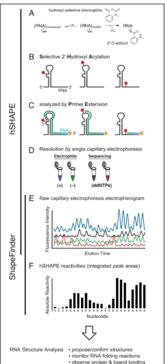
Figure 2.1. Overview of high-throughput Selective 2'-Hydroxyl Acylation analyzed by Primer Extension (hSHAPE) and data processing using ShapeFinder. ..14

Figure 2.2. ShapeFinder at the Align and Integrate stage ...17

Figure 2.3. Electropherogram analysis as implemented using ShapeFinder tools ...20

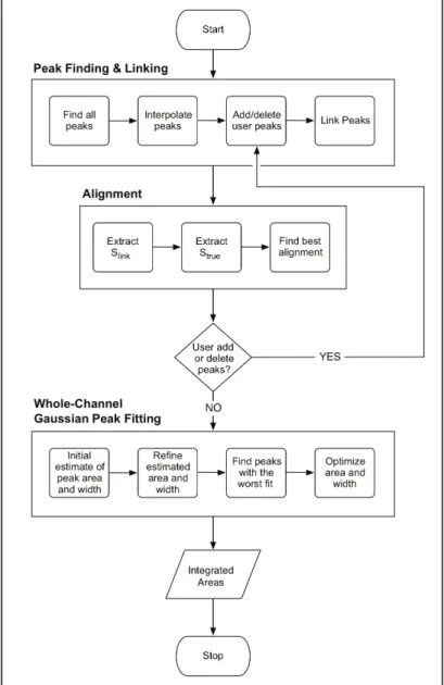
Figure 2.4. Flow chart of the Align and Integrate algorithm ...25

Figure 2.5. Whole-channel peak integration ...29

Figure 2.6. Overview of a complete hSHAPE data set ...30

Figure 2.7. Accuracy and reproducibility of hSHAPE and ShapeFinder...33

Figure 2.8. Peak finding...42

Figure 2.9. Sequence alignment...44

Figure 3.1. Block diagram of steps involved in determining RNA secondary structure using SHAPE...49

Figure 3.2. Alignment captured from the algorithm...52

Figure 3.3. An example of a global alignment ...55

Figure 4.1. Reaction of electrophiles with the 2'-hydroxyl position in RNA...59

Figure 4.2. Box plot analysis of SHAPE reactivities for the entire denatured RNA dataset...62

Figure 4.3. Differential reactivity of unpaired (un) and internally (int) paired nucleotides towards NMIA and 1M7...65

Figure 4.4. Box plots of nucleotides that are single stranded in natively folded RNAs ...66

(12)

Figure 5.1. Bistable switching in bacteria ...77

Figure 5.2. Regulation of competence by a bistable circuit centered on ComK ..79

Figure 5.3. Intracellular model where model starts with the same initial concentrations but agents are placed randomly in the environment ...84

Figure 5.4. The multi-scale agent based model of competence, representing both the intracellular pathways (bottom) and the multicellular environment (top) 86 Figure 5.5. Growth curve of modeled cell culture ...88

Figure 5.6. By following the life cycle of one cell and its progeny, one can see a pattern of inheritance of ComK transcripts and proteins ...91

Figure 5.7. 2-D random walk ...104

Figure 6.1. Mock-up of BKV entry into a salivary gland cell. ...114

Figure 6.2. Biological and computational model of the BKV Life Cycle ...115

Figure 6.3. Boids rules...119

Figure 6.4. A) BKV circular DNA genome depicting the regulatory (RR), early and late regions and transcripts produced ...121

Figure 6.5. Snapshots of agents in a simulation...122

Figure 6.6. in vitro and in silico results showing transcript (VP1 and Tag), protein (Tag), genome and BKV particle concentrations in salivary gland cells...123

(13)

List of Abbreviations

ABM – Agent-based model BKV – BK Virus

CER – Cytoplasm/Endoplasmic Reticulum DNA – Deoxyribonucleic Acid

HIV – Human Immunodeficiency Virus ODE – Ordinary Differential Equations RNA – Ribonucleic acid

SGD – Salivary Gland Disease

(14)

Chapter 1 Introduction

A biological organism is a complex system of multiple interacting molecular pathways comprised of numerous biochemical interactions. Self-organization or complexity in biology occurs through seemingly simple biochemical interactions that give rise to complex patterns and phenotypes such as stripes on a zebra, bacterial phenotypes or viral capsid assembly [1, 2]_{. These not easily predicted biological} patterns manifest over time from seemingly simple interactions, Figure 1.1. Modeling the underlying complexity of these biological patterns remains a challenge and can be quite daunting. Approaches to dissect the biology of a cell range from the study of a specific molecule to the study of gene and protein interaction networks in an

(15)

Figure 1.1. Simple interactions between molecules lead to the expression of different phenotypes.

Instead of modeling individual components, my work attempts to find a

balance between simplification and complexity of biological systems by modeling the simple biochemical interactions. These simple interactions result in the emergence of a global phenotype or complex structures. First, simple interactions between nucleotide bases of the HIV-1 genome were studied to solve its secondary structure. Second, simple interactions involved in a gene regulatory network were modeled to unravel the sources of variability in the expression of the competence phenotype of the gram-positive bacteria Bacillus subtilis. Lastly, the interaction of host cell

machinery with the viral replication and assembly process of BK virus was studied to comprehend the pathogenesis of BKV within salivary gland cells.

1.1 Simple Interactions of a Single Molecule, HIV-1 Genome

Most RNAs perform their biological function(s) only after they fold to form two and three-dimensional structures, Figure 1.1. As an RNA forms a preferred

secondary or tertiarystructure, a subset of nucleotides becomes conformationally constrained by the simple interaction of bases pairing and tertiary interactions, while

(16)

function of the HIV genome is tightly linked to its structure in terms of conformational changes during the progression of infection while interacting with transcription

factors, replication complexes and structural proteins during transcription, replication and packaging [5]. For instance, the structure of the primer binding site (PBS) as seen in Figure 3.1 undergoes a conformation change when the tRNA primer binds to the large loop region [6]_{. This binding stabilizes the tRNA primer, which then is} incorporated into viral particles and is necessary for the initiation of reverse transcription [4].

I developed a software system to aid in secondary structure prediction of an RNA in order to help identify biological function of domains of the HIV genome as described in Chapters 2-4. The software takes a chromatogram of a Selective 2'-Hydroxyl Acylation analyzed by Primer Extension (SHAPE) experiment [6-8]. The cDNA products from each reaction are combined and separated on an automated capillary electrophoresis instrument of the type commonly used for high-throughput DNA sequencing. A single SHAPE experiment measures backbone flexibility of more than 300 RNA nucleotides at a time; multiple experiments can be combined for the analysis of RNAs of any length. The quantified results can then be used as input to third party secondary structure prediction algorithms.

SHAPE provides valuable information about local backbone flexibility, but quantifying the per nucleotide flexibility information is a difficult, time-consuming task. rnafit, a software tool to aid this process, is a command line application that processes SHAPE experiments by aligning sequencing peaks with the RNA

(17)

shows example output from rnafit. Previously, users would search through this output to determine peak finding accuracy and sequence alignment accuracy. To provide a more user-friendly, graphical user interface (GUI) and to provide a more integrated signal-processing platform, I integrated rnafit into BaseFinder and created additional signal processing tools. BaseFinder is a software system originally

designed to analyze spectral data output from DNA sequencing equipment [9]_{. It is} based on an extensible, modular software architecture that easily allows the addition of new analysis algorithms in the form of "tools".

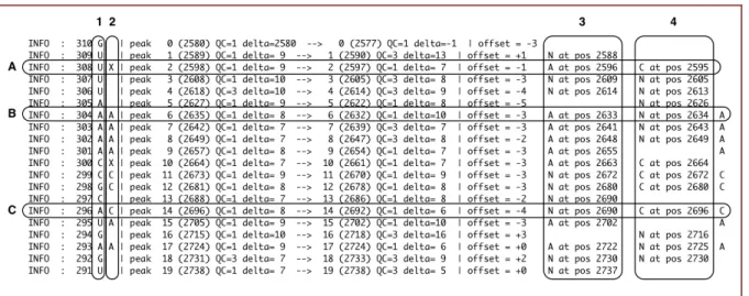
Figure 1.2 rnafit version 0.82 output. Column 1 is the RNA sequence. Column 2 is the aligned sequence. Columns 3 and 4 give feedback on the alignment of the sequencing lanes. A), B) and C) give examples of alignment and misalignment. An X indicates the algorithm was uncertain of the nucleotide in the alignment.

I created a new tool called Align and Integrate that incorporated the rnafit

algorithm, described in Chapter 2. In addition, I performed the statistical analysis as well as create the new signal processing tools of Scale Factor, Mobility Shift: Cubic

(18)

Chapter 3 details improvements I developed for the sequence alignment algorithm of the original rnafit software integrated within the Align and Integrate tool.

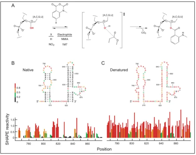
Lastly, there are two published reagents which bind to the 2'-OH of a nucleotide used in SHAPE chemistry: N-methylisatioic anhydride (NMIA) and 1-methyl-7-nitroisatoic anhydride (1M7) [7, 11]. However, a detailed statistical analysis was needed to determine whether or not the reagents exhibit sensitivity to base identity. In other words, do the reagents react equally independent of nucleotide type? Thus, a series of experiments were performed to obtain denatured SHAPE reactivity data of four different RNAs: 976 nts from the 5' end of the HIV-1 genome, the 154 nt specificity domain of Bacillus subtilis RNase P, and ~400 nt internal segments of the Escherichia coli 16S and 23S rRNAs. Both NMIA and 1M7 data was obtained for each RNA and the statistical analysis was performed using a Bootstrap ANOVA detailed in Chapter 4 [12].

Bootstrapping [13, 14] is based on the theory that even though the distribution of the population our data was collected from is unknown, the empirical distribution is a close approximation. Essentially, I estimated the true distribution by repeated

(19)

1.2 Simple Interactions of a Gene Regulatory Network, Competence in B. subtilis

The study of a single molecule does not provide significant insight into the complex interactions involved in gene regulatory networks, but is useful to identify function and interaction partners. Many proteins, RNAs and enzymes interacting with one another lead to the emergence of phenotypes and patterns in nature, Figure 1.1. Following this principle, I modeled a gene regulatory network in order to understand the stochastic nature of the emergence of differing phenotypes in genetically identical bacteria cells. I selected to model the competence gene regulatory network of Bacillus subtilis as described in Chapter 5 as it is a well-studied phenomenon.

Genetically identical bacterial cell populations can express various

phenotypes due to stochastic events and environmental input [15]. There is a growing body of evidence demonstrating that transitions from one bacterial cell phenotype to another are often governed by regulatory feedback loops [16]. This is called bi-stable switching where we have a system with two states, enabled or disabled.

In a B. Subtilis cell, a bi-stable switch controls the competence phenotype that enables the uptake of DNA from the environment. Approximately, 10-20% of a B. subtilis population will express the competence phenotype [17]_{. The metabolic} pathway that enables the competence switch is controlled by cell density and nutritional status and it is highly regulated [17]_{. It has been shown that the random} expression of the competence phenotype is due to the variable expression of the

(20)

Identifying the mechanisms that lead to the random expression of the comK gene is difficult to identify experimentally and the agent-based model (ABM) I created helps visualize this process in order to understand the operation of this system.

In Chapter 5, I describe an ABM of the metabolic pathways that control the competence switch in B. subtilis to study the simple interactions of proteins and other molecules that comprise a gene regulatory network. At the lowest level, my B. subtilis cell ABM, agents represent the proteins and regulatory elements of the competence metabolic pathway. A virtual 3-D environment is created where an agent diffuses throughout the cell landscape and is influenced by random

interactions with other agents. When an agent “bumps” into another agent, rules for interaction between agents are exercised when applicable, such as dimerization, protein binding, transcription, translation, protein or mRNA degradation, etc. The ABM easily models the stochastic events in the molecular pathway, thus, allowing observations on the emergence of competence phenotypic behavior.

At the next level, colony growth by cell division is then modeled by

considering each “Cell ABM” as an agent. Changing nutrient levels in the model and colony growth influence each cell agent’s metabolic pathways such that the

(21)

1.3 Simple Interactions of Interacting Organisms, Virus-Host Cell

Finally, modeling interacting biological networks is another method of understanding how complex patterns, motifs or modules arise from simple biochemical interactions. In the case of virus-host cell interactions, I describe in Chapter 6 a model of the interaction between two organisms to study the emergence of disease.

It is well established that viruses have cell transforming properties and can induce tumor formation and diseases [4]. One such virus is the BK Virus (BKV). BKV, a polyomavirus family member, is a non-enveloped, small, double-stranded DNA virus. BKV is believed to cause a harmless latent infection in healthy people but may reactivate if the immune system has been compromised [19]_{. Recently, BKV has} been detected in HIV positive patients with HIV associated salivary gland disease (HIV SGD) and shown capable of reproducing in salivary gland cells [20]. As salivary gland diseases such as HIV SGD or Sjögren’s Syndrome do not have a known etiological agent, I developed a computational model to pursue this relationship with BKV.

(22)

This model focused on the synthesis of the capsid proteins and self-assembly of the BKV virion to capture viral rates of production. Host cells essentially

(23)

Chapter 2 ShapeFinder: A software system for high-throughput

quantitative analysis of nucleic acid reactivity information

resolved by capillary electorphoresis

2.1 ABSTRACT1

Analysis of the long-range architecture of RNA is a challenging experimental and computational problem. Local nucleotide flexibility, which directly reports

underlying base pairing and tertiary interactions in an RNA, can be comprehensively assessed at single nucleotide resolution using high-throughput selective 2'-hydroxyl acylation analyzed by primer extension (hSHAPE). hSHAPE resolves structure-sensitive chemical modification information by high-resolution capillary

electrophoresis and typically yields quantitative nucleotide flexibility information for 300-600 nts per experiment. The electropherograms generated in hSHAPE

experiments provide a wealth of structural information; however, significant algorithmic analysis steps are required to generate quantitative and interpretable data. We have developed a set of software tools called ShapeFinder to make possible rapid analysis of raw sequencer data from hSHAPE, and most other classes of nucleic acid reactivity experiments. The algorithms in ShapeFinder (1) convert measured fluorescence intensity to quantitative cDNA fragment amounts, (2)

(24)

correct for signal decay over read lengths extending to 600 nts or more, (3) align reactivity data to the known RNA sequence, and (4) quantify per nucleotide reactivities using whole-channel Gaussian integration. The algorithms and user interface tools implemented in ShapeFinder create new opportunities for tackling ambitious problems involving high-throughput analysis of structure-function relationships in large RNAs.

2.2 INTRODUCTION

An absolute prerequisite for understanding the function of any RNA is an accurate picture of its higher order structure. Analysis of in-solution nucleic acid structural information often requires that RNA or DNA fragment lengths be analyzed at single nucleotide resolution. Important examples in this class include

"footprinting", chemical modification and modification-interference experiments [8, 21-25]_{These experiments can be performed in a wide variety of ways designed to}

analyze local nucleotide conformational differences, solvent accessibility, and the effects of functional group modifications on RNA and DNA folding and interactions with protein and small molecule ligands. For over three decades, these classes of experiments have been evaluated by resolving nucleic acid fragments on

polyacrylamide slab gels [26]. Gel electrophoresis has significant advantages including good nucleotide resolution of nucleic acid fragments and low material costs. However, gel electrophoresis is time consuming, single nucleotide-resolution separation is typically limited to 80-100 nts per gel, and band overlap and

(25)

In contrast to the limited read lengths obtained by gel electrophoresis, commercially available capillary electrophoresis instruments of the type commonly used for DNA sequencing routinely yield read lengths of 300 to 1000 positions at single nucleotide resolution. However, the absence of an appropriate set of software algorithms that address the unique quantitative properties of raw electropherograms generated by structure-probing experiments has prevented the use of capillary electrophoresis for high-throughput, single-nucleotide resolution, analysis of nucleic acid folding, dynamics, and ligand binding.

To address this problem, we have created a new software suite called ShapeFinder that automates the steps required to extract quantitative, single nucleotide resolution reactivity information for 300-650 nts in a single capillary electrophoresis run. We focus here on the analysis of SHAPE (selective 2'-hydroxyl acylation analyzed by primer extension) experiments [7, 8, 27]. However, the

algorithms created in this work can also be used to analyze raw capillary electrophoresis data from other classes of nucleic acid reactivity experiments, including those that use other chemical modification agents or hydroxyl radicals to map structure and solvent accessibility (unpublished data).

2.2.1 RNA Structure and hSHAPE Chemistry.

(26)

exquisitely sensitive to local nucleotide flexibility [7]_{(Figure 2.1A). Nucleotides that} are constrained by base pairing or tertiary interactions are unreactive, while

conformationally flexible (and likely single-stranded) nucleotides preferentially form 2'-O-adducts (Figure 2.1A,B). Sites of modification are located by annealing a 5'-end labeled primer to the RNA and then ext5'-ending the primer to the nearest site of modification using reverse transcriptase in an optimized primer extension reaction [7, 8]_{. The product of this experiment is a series of extended, 5'-end labeled cDNA}

fragments whose length and amount correspond to the position and degree of modification -- and hence local nucleotide flexibility -- at every nucleotide in an RNA (Figure 2.1C). In order to assess RNA degradation and position-dependent

processivity of the primer extension reaction, a control omitting the reagent is performed in parallel. Third, in addition to the (+) and (–) reagent reactions, one or two dideoxy sequencing reactions are used to map reactivity to the RNA sequence (Figure 2.1D).

(27)

are complex and require substantial processing before they can be used to infer RNA structural information.

(28)

2.2.2 Algorithmic Challenges for Nucleic Acid Structure Analysis Resolved by Capillary Electrophoresis.

The output of an hSHAPE experiment resolved by capillary electrophoresis is an electropherogram, or trace. A typical trace contains 3 to 4 individual channels of fluorescence intensity versus elution time data; where each channel roughly

corresponds to one of the SHAPE reactions (Figure 2.1E). The results of hSHAPE and DNA sequencing experiments resemble each other in that both experiments generate a series of measured fluorescence intensities versus elution time and must be processed extensively in order to yield useful nucleotide resolution information. However, extracting reactivity versus nucleotide position information for an hSHAPE or any other nucleic acid reactivity experiment requires the use of unique algorithms and data processing strategies.

The first and most important difference is that peak magnitude in DNA

sequencing contains little meaning other than to indicate which nucleotide is present at a position. In contrast, both peak intensity and position are meaningful for all peaks in the (+) and (–) reagent channels in an hSHAPE experiment. Peak intensity spans a dynamic range of 50-fold and reports the structure-sensitive yield of the

2'-O-adduct, and thus local nucleotide flexibility (Figure 2.1A). The position reflects the length of the extended primer, and hence the nucleotide position in the RNA.

Critically, the processing steps applied to hSHAPE data must not disturb relative intensity or distribution features of peaks in the electropherogram.

(29)

experiment. Thus, hSHAPE peaks must be aligned with each other with greater precision because quantitative analysis of reactivity information requires greater alignment accuracy and it is not possible to base alignment on the expectation that there is only one intense peak per trace position.

Third, peak position and area must be determined for every position in the (+) and (–) reagent channels to quantify nucleotide reactivity; whereas, sequencing only requires locating the most intense peak per position. Importantly, the absence of a peak in the (+) reagent channel in an hSHAPE experiment represents significant information and indicates that a nucleotide is constrained by base pairing or tertiary interactions. Thus, accurate identification and quantitative analysis of noisy, barely detectable, peaks is an absolute requirement for successful hSHAPE analysis. Finally, fully automated analysis of hSHAPE data requires that sparse sequencing data be aligned to a known input sequence. This is the opposite of DNA

sequencing, where the goal is to determine a precise sequence of nucleotides.

2.3 RESULTS

2.3.1 ShapeFinder

The initial processing steps required to convert raw capillary electrophoresis profiles into useful reactivity information are similar to those involved in analysis of DNA sequencing traces. We therefore extended the BaseFinder platform[9], a framework originally designed for DNA trace processing, analysis and base-calling, for analysis of nucleic reactivity information as resolved capillary electrophoresis. ShapeFinder is a modular, extensible software package in which each

(30)

immediately displayed to the user in a straightforward graphical user interface (Figure 2.2).

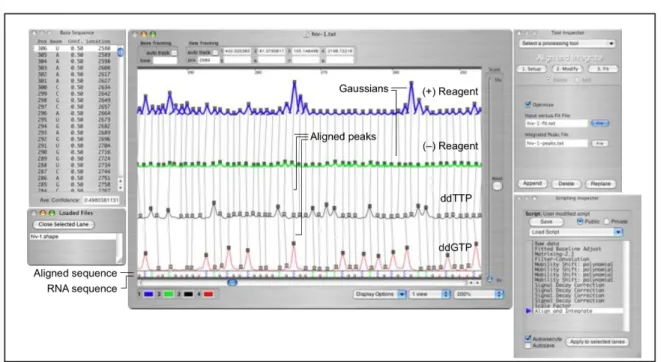
Figure 2.2. ShapeFinder at the Align and Integrate stage. The Data View Window (center) provides graphical feedback on each data processing step. The Tool Inspector window (upper right) displays the user-definable parameters for the tool selected in the Scripting Inspector. The Scripting Inspector (lower right) displays the tools thus far applied to the data.

ShapeFinder reads and displays files from most common sequencing

platforms, including generic tab-delimited .txt files, the Beckman .esd and .dat files, and the ABI .fsa, .abi, and .ab1 formats. ShapeFinder also implements a new file format (.shape) that stores the raw and processed hSHAPE data along with the tool parameters that have been applied to the data set. The .shape file allows for review and re-execution of trace processing steps and facilitates testing the effects of different parameter choices.

(31)

used in numerous ways in the analysis of nucleic acid reactivity experiments. In the case of an hSHAPE experiment, reactivity information has thus far been used to develop models for an RNA secondary structure, to monitor RNA folding reactions, and to evaluate the effects of protein binding and macromolecular complex formation [6, 11, 38]_.

2.3.2 ShapeFinder Tools

ShapeFinder implements the algorithms required to convert raw capillary electrophoresis electropherograms into useful reactivity information through the execution of a specific sequence of tools, called a script. Each tool in a script

accomplishes a specific data processing step by applying user-definable parameters to the electropherogram. The current script is displayed in the Scripting Inspector window in the ShapeFinder user interface (Figure 2.2, lower right). Tools are added and run using the Tool Inspector window, which also displays the parameter values associated with each tool (Figure 2.2, upper right). A processing tool is added using the "Append" button; tools already in a script may be changed and rerun by selecting "Replace." An individual step and its associated parameters may be reviewed by selecting the tool entry in the Scripting Inspector window.

Complete analysis of an hSHAPE raw capillary electrophoresis profile

(32)

the (+) and (–) reagent channels are identified and linked to the input RNA

sequence, including those "peaks" corresponding to zero reactivity (peak alignment). Finally, quantitative nucleotide reactivities are obtained by performing a

whole-channel Gaussian integration for all peaks in the (+) and (–) reagent whole-channels (peak integration). Subtracting the integrated values for the (–) reagent from the (+)

reagent profiles yields the absolute nucleotide-resolution reactivity for every RNA position over read lengths typically spanning 300-600 nts. An experienced individual can perform the data processing steps in approximately 1-2 hours.

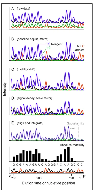
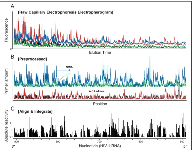
We will illustrate these processing steps using an experiment performed on a transcript corresponding to the first 976 nts for the NL4-3 strain of the HIV-1

(33)

Figure 2.3. Electropherogram analysis as implemented using ShapeFinder tools. (A) Unprocessed capillary electrophoresis electropherogram. (B) Net result after

(34)

2.3.3 Data Preprocessing

Fitted Baseline Adjust, Matrixing and Smoothing. Channels in raw capillary electropherograms are convoluted by detector background, overlapping emission spectra, detector noise, and horizontal offset between channels (Figure 2.1E, Figure 2.3A, and Figure 2.6A). Since these traits are common to all

electropherogram data, initial processing of the raw electropherograms involves steps analogous to those used for DNA sequencing experiments.

Fluorescent background noise causes the baseline in each channel to drift, which imparts an idiosyncratic vertical offset to each channel. The Fitted Baseline Adjust tool adjusts each channel to a common baseline by zeroing each channel over a window of detector readings, typically ten times the average peak width.

(35)

Trace data from a DNA sequencer contains fluctuations due to detector noise so that each major peak may have minor peaks and valleys of its own, which

complicates downstream peak finding. Smoothing can increase read length and peak detection by ~10% for datsets with low signal to noise ratios. The result of the Baseline Correction, Matrixing and Smoothing tools on the HIV-1 NL4-3 transcript are shown in Figure 2.3B.

Mobility Shift. In an hSHAPE experiment, each reaction is analyzed using a DNA primer labeled with a different fluorophore (Figure 2.1D). The dyes alter the electrophoretic migration rate of the cDNA products so that cDNAs of the same length have slightly different elution times (Figure 2.3B). For hSHAPE data, correction for mobility shifts must be performed more accurately than is generally required for DNA sequencing to facilitate accurate location and linking of

corresponding peaks between channels. ShapeFinder implements several mobility shift tools that can be combined in serial to account for horizontal offset without significantly altering peak shapes. Two to four serial applications of the Mobility Shift: Cubic tool typically places all channels on a consistent x-axis (Figure 2.3C).

Parameters for an initial mobility shift must be set once for each set of primers. These parameters can also be fine-tuned on a trace-by-trace basis.

(36)

adding an additional nucleotide to a cDNA is slightly less than one. (2) The (+) reagent reaction is designed that, on average, only one in every 300 nts is modified. However, because modification is random over long RNA lengths, some RNAs react two or more times. For RNAs containing multiple adducts, only the first site of

modification is detected, thus favoring short cDNAs. (3) In the sequencing reactions, the population of extending primers decreases by a small factor each time a

dideoxynucleotide is incorporated. Thus, the signal decays exponentially to zero in all channels at read-lengths of 400-650 nts. This decay is also observed in DNA sequencing experiments and is corrected by normalizing peak intensities across all channels to consistent heights [9].

In the case of hSHAPE experiments, fluorescence intensity is meaningful, so the decay correction must be performed using a statistical model of signal decay. We find that signal decay is well modeled as:

D(x) = Aqx + C (1)

where D is the signal intensity as a function of primer elongation, A is the amplitude of the decay, C represents the measured intensity at the end of the channel, and q is the probability of extension at position x[30].

(37)

Scaling. Experimental variations in performing primer extension, inherent differences in dye intensity (compare black and red channels, Figure 2.6A) and second-order effects of the ShapeFinder Smoothing and Signal Decay Correction tools can cause the channels to be on different scales. The channels are adjusted manually such that the smallest 5-10% of the peaks throughout the (+) channel match corresponding (–) channel intensity (Figure 2.3D, compare blue and green channels). This correction assumes that there are always a few completely unreactive nucleotides in an hSHAPE read whose peak intensities should exactly match the corresponding (–) peak intensities. For ease in data viewing and further analysis, sequencing peaks are set to match moderately intense peaks in the (+) channel (Figure 2.3D, compare red and black to blue channels). After preprocessing, all channels have a baseline set to zero, peaks in different channels corresponding to the same nucleotide have the same elution time, and well-defined peak intensities correspond quantitatively to cDNA amounts (Figure 2.3D).

2.3.4 Whole-Channel Peak Alignment and Integration

(38)

Modify panel allows the user to add and remove peaks in phase 3; and the Fit panel is used to manage phase 4. The tool is iterative and alignments are recalculated after each round of user input. Subtracting the (–) from the (+) reagent peaks is performed automatically and yields absolute hSHAPE reactivities for every nucleotide in the capillary electrophoresis read (bars, Figure 2.3E).

(39)

Primer extension stops at the base preceding the nucleotide containing a

2'-O-adduct; thus, the (+) and (–) reagent peaks are one nucleotide longer than the cDNA fragments generated by dideoxy sequencing [7]. Therefore, the sequencing alignment is shifted by one nucleotide relative to the (+) and (–) reagent channels. To avoid confusion, the ShapeFinder display shows the sequencing peaks without an offset. Text output files show the offset.

Setup. In the Setup phase, the user assigns each channel to one of the four SHAPE reactions [(+) and (–) reagent, and sequencing ladders] and specifies the region of the trace to be analyzed using either numerical trace positions or by selecting a region of the trace in the main window. A Refine option enables

automatic interpolation of peaks in the (+) reagent or (–) reagent channels based on the expected spacing in a given region of the trace. The Setup phase also reads a text file containing the RNA sequence in the 5' to 3' direction that is used to align the trace data to the RNA nucleotide position.

A preliminary alignment is initiated after these parameters have been set. The data view window displays the four channels and demarcates identified peaks with squares (Figure 2.2). Vertical lines show peaks in the four channels that have been linked with each other and with the input sequence. Light-shaded squares in either the (+) or (–) reagent channels indicate unlinked peaks. For the sequencing

channels, light-shaded squares report peaks that were identified but were not accepted as part of the sequencing ladder.

Modify. In portions of a run with strong signal, low-noise, and good

(40)

in some regions, especially near the ends of a read, meaningful peaks may be missed, not aligned, or assigned incorrectly. However, these regions often contain high quality and quantitative SHAPE structural information that can be gleaned with operator supervision. To this end, ShapeFinder allows manual editing and extension of the automatically generated alignment using the Modify panel (illustrated

schematically in Figure 2.4).

The ShapeFinder-determined sequence alignment is displayed at the bottom of the data window (Figure 2.2). The top sequence is determined from the

sequencing channels, while the bottom sequence shows the loaded sequence. For completely aligned data, letters coincide vertically between the two datasets. When the data are partially misaligned relative to the input sequence, there will be a horizontal offset between the two sequences. The addition or deletion of a peak in the (+) reagent channel is usually required to correct the alignment. Finding the location of a missed or incorrectly added peak is accomplished in a straightforward way by locating the position where horizontal offset begins.

Peaks to be deleted or added are selected by clicking on the square at the top of each peak, or clicking at the desired position for a new peak in any channel, respectively. The tool window displays a spreadsheet-style list of peak positions that have been added or deleted (left panel, Figure 2.2). Data that is ready for Gaussian fitting (center, Figure 2.2) is correctly aligned to the sequence and has all (+) and (–) peaks linked to each other and to the sequence, as indicated by filled boxes.

(41)

unalignable regions may be removed in the Setup panel by adjusting the Trace Range. For the HIV-1 example dataset, three unaligned (+) reagent peaks were deleted at the beginning of the trace. This correction then allowed complete alignment of >400 continuous nucleotides in the RNA.

Fit. Once all peaks to be analyzed have been identified and linked with the input sequence, the Fit phase of the Align and Integrate tool performs whole-channel Gaussian peak integration for the (+) and (–) reagent channels (Figure 2.3E). Each peak is fit to

(2)

where A_{i is the peak area and}µ_{i and}σ_{i are the center and width of peak}i,

respectively. The tool has both fast and optimize modes. The Optimize option provides a more accurate peak fitting, but is more computationally demanding (Figure 2.5).

Once fitting is complete, ShapeFinder displays the calculated peaks superimposed upon the (+) and (–) reagent channels in the data view window

(Figure 2.2, bold lines). The fitted Gaussian curves for all peaks, the calculated peak areas, the net absolute reactivity at every position, the alignment to the input

(42)

Figure 2.5. Whole-channel peak integration. (A) Preliminary local fit to initialize values for Ai and σi. (B) Final globally optimized fit.

2.3.5 Example of a Complete hSHAPE Experiment, Quantified by ShapeFinder A complete hSHAPE electropherogram contains structural information for several hundred RNA nucleotides (Figure 2.6A). As outlined above, the raw data for the HIV-1 example RNA includes all of the typical characteristics of raw

(43)

set to zero, peak intensities correspond quantitatively to cDNA amounts, and overall peak heights are distributed evenly throughout each channel (Figure 2.6B).

Figure 2.6. Overview of a complete hSHAPE data set, processed using

ShapeFinder and representing a total read length of 415 nts from an HIV-1 transcript RNA. (A) Raw electropherogram from a DNA sequencer. The data consists of four channels of fluorescence intensity information as a function of elution time. (B) Preprocessed SHAPE data. Each channel now represents dye amount, not

fluorescence, as a function of elution time for each of the four channels. For clarity, channels corresponding to the A and C sequencing ladders are offset from the (+) and (–) reagent channels. (C) Sequence alignment and whole-channel Gaussian peak integration using the Align and Integrate tool to calculate absolute SHAPE reactivities.

(44)

and (–) channels by whole-trace Gaussian integration. Subtracting the (–) peak areas from the (+) reagent peaks yields the absolute hSHAPE reactivity for every nucleotide in the capillary electrophoresis electropherogram (bars, Figure 2.6C). In this typical experiment, single nucleotide resolution SHAPE reactivities were

obtained for positions 491–905 in the HIV-1 transcript, for a total read length of 415 nts.

2.3.6 Analysis of Accuracy and the Reproducibility of hSHAPE and ShapeFinder

(45)

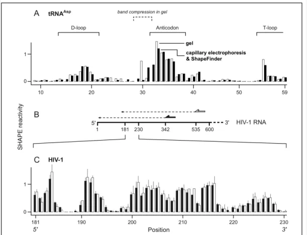
Inspection of the two datasets indicates that quantitative analysis of cDNA fragments obtained from a SHAPE analysis of the tRNAAsp transcript yielded nearly identical reactivities at almost all positions, regardless of the separation and analysis platforms (compare solid and open columns, Figure 2.7A). The linear relationship correlation coefficient, R, between the two datasets is 0.91, indicating 83% (R2) of the variability of the hSHAPE data can be predicted by the variability of the gel data. This correlation is significant at the p < 0.0001 level. Comparison of the differences in reactivities between the two datasets yielded a Student t-test p-value of 0.84, indicating the group reactivities are statistically equivalent.

The only significant differences in measured nucleotide reactivity occurred at positions 29-32. The differences reflect the difficulty in calculating intensities in the context of band compression that occurs when cDNA fragments for this RNA are resolved by gel electrophoresis [27, 40] (labeled, Figure 2.7A); these positions were therefore not included in the correlation analysis. In contrast, positions 29-32 were readily interpretable in the capillary electrophoresis trace. Thus, ShapeFinder yields quantitative values for per nucleotide reactivities that are as accurate as the

conventional approach using gel electrophoresis. The only difference is that capillary electrophoresis is less sensitive to band compression artifacts.

(46)

arrows, Figure 2.7B). The overlapping regions therefore also correspond to sets of peaks that have been differentially adjusted by the Signal Decay Correction

algorithm.

Figure 2.7. Accuracy and reproducibility of hSHAPE and ShapeFinder. (A)

Comparison of nucleotide reactivity as quantified by ShapeFinder (closed bars) and denaturing gel electrophoresis (open bars). Loops in tRNAAsp_{are indicated}

explicitly. The tRNAAsp sequence was flanked by 5' and 3' structure cassette sequences [7]. Due to strong band compression [27, 40], some positions cannot be visualized by gel electrophoresis. Bands visualized by gel electrophoresis were quantified using SAFA [39]. (B) Overlapping reads for HIV-1 genome transcripts. Primers, shown as solid and open arrows, anneal to the RNA 193 nts apart and reads therefore overlap by ~200 nucleotides (dashed lines). (C) Mean hSHAPE reactivities and standard deviations calculated from overlapping and replicate reads. Primers annealed at positions 342-363 (solid columns) and 535-555 (open columns). Data shown report three experiments from the 342-363 primer and two experiments from the 535-555 primer for five experiments total, whiskers report standard

(47)

We performed several statistical tests to evaluate how similar calculated peak intensities are across data sets. Correlation coefficients calculated between the 10 possible pairs of the 5 datasets indicated a very strong correlation between the datasets, with R2 values ranging from 0.86 to 0.97 (p-values < 0.0001). A one-way ANOVA (analysis of variation) performed between the 5 datasets showed the SHAPE reactivities to be statistically equivalent (p = 0.77). Furthermore, Levene’s Test indicated constant variance between the five datasets (p-value = 0.26). Finally, we calculated the standard deviation for each measurement in the 181-230 window. A plot of the per position standard deviation as a function of mean SHAPE reactivity is linear (R = 0.73; p < 0.0001). Linear regression indicates that the average

measurement error at any one nucleotide is 0.04 + 0.11 × (per position

measurement) in SHAPE units. Thus, for representative low and high SHAPE reactivities of 0.1 and 0.7, measurement errors are expected to be ±0.05 and ±0.12 SHAPE units, respectively.

In sum, these statistical tests indicate that SHAPE reactivities as quantified using ShapeFinder (i) are calculated accurately over hundreds of nucleotides, (ii) are accurately corrected for signal decay as modeled by Eqn. 1, and (iii) exhibit small absolute measurement errors. Combining quantitative reactivities from individual reads of 300-650 nts can therefore robustly monitor the structures of long RNAs, potentially spanning thousands of nucleotides.

2.4 Discussion

(48)

and ligand binding for RNAs of known structure, and for developing models for RNAs whose structures are not known. A critical limiting step in such analyses has been the use of gel electrophoresis technology to visualize the results of these experiments. In many cases, more effort is required to obtain, manipulate, and quantify information by gel electrophoresis than is spent actually performing the experiment or interpreting its result.

The algorithms implemented in ShapeFinder dramatically lower the barriers to monitoring the structure of large RNAs. Depending on the characteristics of an RNA, we routinely obtain read lengths of ~400 nts, with reads of up to 650 nts under optimal conditions. This means that single nucleotide resolution structure

information can now be obtained for entire large catalytic and regulatory RNAs or domains of larger RNAs like ribosomal RNAs in a single experiment.

While ShapeFinder accelerates the ability to interrogate RNA structure in solution at single nucleotide resolution, we are continuing to develop new methods and algorithms to further improve the speed, accuracy and automation of hSHAPE analysis. Important objectives include improved and automatic mobility shift

(49)

2.5 MATERIALS AND METHODS

2.5.1 SHAPE Data.

SHAPE experiments were performed on an HIV-1 transcript or tRNAAsp exactly as described [6, 7]. Most of the SHAPE reactivity data on HIV-1 sequences presented here was reported previously [6]. Briefly, DNA templates encoding the 5'-most 976 nts of the HIV-1 NL4-3 strain (Gen Bank AF324493) or tRNAAsp were generated by PCR. The RNA construct was produced by in vitro transcription and purified by gel electrophoresis. The HIV-1 RNA and tRNAAsp_{(1 pmol) were refolded} in 50 mM HEPES (pH 8.0), 200 mM potassium acetate (pH 8), and 5 mM MgCl2; or 100 mM HEPES (pH 8.0), 100 mM NaCl, 10 mM MgCl2, respectively, at 37 ˚C for 30 min. (+) and (–) reagent SHAPE reactions were initiated by treating the RNA with N-methylisatoic anhydride (NMIA, 32.5 mM in DMSO) or DMSO, respectively. After the NMIA hydrolyzed completely (60 min) [7]_{, the RNA was recovered by ethanol}

precipitation and mixed with fluorescently labeled DNA primers (Proligo or LI-COR) that annealed at either positions 342-363, 535-555 or 956-976. Primer extension was initiated by addition of Superscript III reverse transcriptase (Invitrogen). Sequencing markers were generated using unmodified RNA by performing primer extension in the presence of dideoxy NTPs. Dyes for the (+) and (–) reagent and sequencing lanes were Cy5, WellRed D3, WellRed D2 and LI-COR IR 800, respectively. cDNA products from the four reactions were mixed, purified, and separated on a Beckman CEQ2000XL capillary electrophoresis DNA sequencer. tRNAAsp experiments were performed both using a 5'-radiolabeled primer and resolving primer extension fragments on electrophoresis gels [7, 27]_{or using}

(50)

the same manner as HIV-1, except that 130 mM NMIA was used. Fluorescence intensity over the 4 channels was monitored at a rate of 2 Hz and yielded an

average of ~10 points per peak position. Raw electropherograms were output from the capillary electrophoresis instrument in the Beckman .txt format and read directly into ShapeFinder.

2.5.2 ShapeFinder Software

ShapeFinder is a derivative of the BaseFinder trace-processing platform and is written in Objective-C [9]. It is distributed as a Universal Binary, and runs on Macintosh PowerPC or Intel computers running Max OS X 10.4 or later.

ShapeFinder is freely available for non-commercial use. A comprehensive Help File is also available in the software package for new users of hSHAPE technology and ShapeFinder. Both the ShapeFinder software and help package, as well as all HIV-1 data and example scripts used in this work are available at:

http://bioinfo.unc.edu/downloads/.

Fitted Baseline Adjust. The Fitted Baseline Adjust tool calculates a common baseline for each channel while keeping the experimentally recorded data intact [9]. The local minima in a channel are found after dividing the channel into windows representing 5-20 times the average peak width. For the HIV-1 dataset, the window size was 200 because peak widths usually are ~10±5 data points.

(51)

function of position. The transformation matrix is calibrated using four extension reactions run in separate capillary columns, which need be performed only once per dye set. The extension reactions must generate a series of intense, but not

saturating, peaks for each fluorophore, and is most easily achieved by generating sequencing channels. The extension products are resolved in independent capillary runs, such that each electropherogram contains fluorescence from a single dye. The user selects an intense peak for each of the dyes and ShapeFinder automatically calculates a transformation matrix that can be used for all experiments using the same dye set.

Smoothing. Trace data from a DNA sequencer contains fluctuations due to detector noise. The peak-fitting and alignment algorithm implements an internal smoothing step to correct such noise and we find that this smoothing is sufficient for optimal processing in most cases. However, in cases where trace data are very noisy, or the user prefers the displayed data to be smoothed, a separate smoothing step can be applied using the Filter-Convolution [9] tool. Recommended parameters are a Gaussian width σ = 1 and window size of 10. Judicious noise reduction by smoothing is helpful; however, it is important that this step not be overdone or adjacent peaks can blend together.

(52)

to the data. These parameters need be determined only once for a given primer set, but individual electropherograms may require fine-tuning. Two to three iterations of the Mobility Shift: Cubic tool are usually sufficient for an hSHAPE electropherogram.

Signal Decay Correction. This tool corrects the decay in peak intensity due to the stochastic nature of 2'-hydroxyl modification and the imperfect processivity of reverse transcriptase. At each nucleotide position, there is a probability p that a reagent-modified nucleotide will stop reverse transcriptase. The probability that the reaction will continue, q [q = (1 – p)], yields the exponential form observed for peak drop-off that we model with Eqn. 1.

For each hSHAPE experiment, the algorithm determines the best-fit parameters from equation 1 in two steps. First, it identifies peak locations,

calculates their height, and removes outliers. Peaks are identified by considering seven consecutive points, calculating the slope of the line connecting each

sequential pair of neighboring points, and then averaging the six consecutive slopes. Peak maxima are identified as the points where the derivative transitions from

positive to negative. Anomalously high outlier peaks are identified and excluded using a box plot model in which outliers fall outside 1.5 times the inter-quartile range of the data [41]. Second, the algorithm fits the remaining peak heights to Eqn. 2 to determine A, C and q using Levenberg-Marquardt non-linear least squares

(53)

Each channel in the hSHAPE electropherogram is corrected independently for signal decay.

After parameter estimation, the reagent and control channels are then corrected for signal decay using:

I_new(x) = N×I_old(x)/D(x) (3)

where I_{old is the original measured intensity,}D(x) is from Eqn. 1, and N is a

user-definable rescaling factor that maintains overall peak intensity relative to the other non-corrected channels.

Scale Factor. This simple tool is used to rescale individual channels in a trace. This may be necessary because fluorescent intensity values measured in distinct channels depend on the properties of the fluorophores and detector,

resulting in an arbitrary relative scaling between channels. The tool takes the user-specified channel scaling factors and multiplies them against the intensity values for the specified channel, adjusting each channel to be on the same relative vertical scale. Data should be scaled so that peak heights range above 100 (arbitrary) units to improve the accuracy of subsequent peak fitting.

2.5.2.1 Align and Integrate

(1) Peak finding and linking. This first phase accepts user input that specifies (i) which extensions [(+), (–), or sequencing] were performed in each channel, (ii) the region of the preprocessed data to analyze, and (iii) the sequence. The sequence is read from an ASCII-formatted text file where white space

(54)

which cDNAs elute in the 3' to 5' direction with respect to the RNA sequence. Prior to peak finding, data are smoothed over a three-point window (dashed lines Figure 2.8). The algorithm first identifies the peaks in each channel by identifying those that are the highest point centered within a range of ±3 neighboring points. The most frequent distance between peaks is then calculated, and additional peaks

interpolated when the distance between two peaks is greater then the most frequent peak distance (initially identified and interpolated peaks are shown by the open and closed circles in Phase A of Figure 2.8). Since the linearly interpolated location may not lie on a local maximum, interpolated peaks are then shifted left or right to a maximal position [for example, position 2845 in the (+) channel in Phase B of Figure 2.8]. Peaks in the (+) and (–) reagent channels are aligned with each other if they are positioned near each other on the elution time axis, defined by a distance

threshold t that is iteratively incremented from zero to a maximum value k/2, where k

is the median distance between neighboring peaks in the channel. In sum, this algorithm matches the best-aligned peaks first and then incrementally allows for misalignment of peaks that do not initially match (illustrated by lines linking the circles in Figure 2.8). A preliminary alignment for 600 nts requires 2 seconds on a 1.5 GHz Power PC processor.

(55)

deleted. When the Modify option is used to add or delete peaks (see Figure 2.4) the algorithm adds these peaks and automatically creates the appropriate new peaks links (Phase D in Figure 2.8).

Figure 2.8. Peak finding. The electropherogram shows the (+) and (–) reagent channels (blue and green, respectively). The (–) reagent intensities have been inverted and are plotted on an expanded scale to facilitate visualization of peak synchronization. Preprocessed channels are shown as solid lines, channels smoothed over a 3-nt window are dashed. (A) Identification of peak positions by analysis of (i) signal amplitude and (ii) interpolation are illustrated by open and closed circles, respectively. (B) Refinement of interpolated peaks positions. (C) Automatic addition of missing peaks (blue circles) after comparison of the (+) and (–) reagent channels. (D) Incorporation of peaks added (red circles) or deleted by the user and subsequent refinement of peak positions. Positions of synchronized (+) and (–) reagent peaks that will be used during the integration phase are emphasized with solid lines.

(56)

transcriptase and RNA degradation, as well as intense peaks indicating the presence of the sequenced nucleotide. These two classes are separated using a user-definable sensitivity level: peaks are part of the sequencing ladder only if their height is greater than the median channel intensity multiplied by the sensitivity level. By decreasing the sensitivity, more sequencing peaks are identified as part of a sequencing ladder; conversely, by increasing the sensitivity, fewer sequencing peaks are found. In the final step of this phase, sequencing peaks are linked to the (+) and (–) reagent peaks if the peak is within ±2 points on the x-axis of a (+) or (–)

reagent peak (Figure 2.9, Phase C).

(2) Alignment to the RNA sequence. The next step in this algorithm is to align the trace data with the known RNA sequence (see Alignment steps in Figure 2.4). A sequence, Slink, is derived by correspondence of the sequence ladder from the ddNTP channels to the (+) reagent peaks, in which an N indicates the positions of non-sequenced nucleotides and the appropriate A, G, C, or U indicates the linked ddNTP peak. An example sequence for a reaction using ddUTP and ddGTP might be NCAANCNNNCNCAC. A sequence Strue is created from the known RNA

(57)

Consistent horizontal offsets signify an incorrectly identified peak or unidentified peaks and are corrected by editing the alignment.

Figure 2.9. Sequence alignment. Electropherogram showing the (+) reagent (bottom) and the ddNTP (top) channels. Sequencing channels have been inverted to facilitate visualization of peak synchronization with the reagent channel. Reagent peaks assigned in the alignment step (Figure 2.8) are highlighted with blue dotted lines. Results of the four phases of sequence assignment are plotted together with their respective spectra. (A,B) Detection of peaks corresponding to the first and second sequencing channels, respectively. Peaks not accepted as valid sequencing positions are shown with black and red filled circles. (C) Assignment of input

sequence to the identified sequencing peaks. (D) Complete alignment of the input RNA sequence. This alignment is offset by one nucleotide to reflect that dideoxy sequencing fragments are 1 nucleotide longer then the cDNA fragments that identify 2'-O-adduct sites.

(58)

necessary. Generating a correct alignment by adding and deleting peaks is an iterative process.

(4) Whole Channel Gaussian Peak Fitting. Once the alignment is correct, the intensity of each peak in the (+) and (–) reagent channels is quantified by fitting a Gaussian curve to each peak in the entire channel (Eqn. 2). The three variables that characterize each peak are the peak area (Ai) and the center and width of peak i (µ_i

and σ_{i, respectively). Since the center of the peak,}µ_{i, was determined during the}

peak finding phase, this equation has two unknowns for each peak: area, Ai, and

peak width, σ_{i. ShapeFinder implements an exhaustive search algorithm to optimize}

A and σ for each peak. The search algorithm is executed several times, with each

iteration refining the search space for Ai and σ_i.

Initial estimates of Ai and σ_{i for a given peak are calculated from a local}

three-peak Gaussian fit of the target three-peak and the neighboring three-peaks on each side. Initial values of Ai are taken from γ_i/2≤ Ai ≤ 10γ_{i , where}γ_{i is the amplitude of the peak}

fluorescence intensity. σ_{i estimates are taken from the range 0.8}≤ σ_i≤ 4.5. The

estimation is repeated for 16 iterations where the sample space of A is adjusted each round to Ai,best – 0.5Ai,best ≤_Ai≤_{Ai,best + 0.5Ai,best, where Ai,best is the}

area calculation from the previous round which best fit the data. The next iteration of the search algorithm refines estimates for Ai and σ_{i by using a different sample}

space for σ_{i, 0.4}σ_med≤σ_i≤σ_{i + 0.5}σ_{med, where}σ_{med is the peak width median}

(59)

between the experimental and fit intensities, although the peak area is slightly underestimated (Figure 2.5A).

If the Optimize option is enabled, estimates of A and σ are improved further at the cost of increased processor time. New parameters are estimated by sampling Ai

≤_Anew≤_{Ai + 10Ai, and fixing the width,}ω, as the minimum σ_{i computed thus far;}

each σ_{i is retained as}σ_{i,old for the future. As the initial new}ω is taken as the

minimum σ_{i computed so far, the new A estimates are larger to compensate for the}

smaller ω. In the final phase of the Optimize algorithm, peak widths are improved in

two stages. In the first stage, peak widths are optimized by sampling a new σ_{i from}ω

≤σ_i,new≤σ_{i,old, starting with the peak with the worst fit. After each selected peak is}

optimized, then a new peak with the worst fit is determined. This is repeated n times, where n is equal to 3 times the number of identified peaks. In the second stage, the peak with the worst fit is again determined and peak width is optimized by sampling,

σ_i≤ σ_i,new≤ σ_{i + 0.1}σ_{i,old, provided}σ_{i + 0.1}σ_{i,old <}σ_{i,old. The new width is saved}

if it improves the fit, otherwise the old information is retained. Results of this final optimization step are shown in Figure 2.5B. Fitting ~400 nts of the HIV-1 sample data requires ~16 min on a 1.5 GHz Power PC processor versus 3 min with the Optimize option disabled.

(60)

contains a tab-delimited spreadsheet of the calculated peak positions, widths, areas, and RMS errors for the (+) reagent (RX) and (–) reagent (BG) channels, as well as their alignment to the target RNA sequence. This file also contains a column where the (–) peak areas are subtracted from their corresponding (+) peak areas to

determine absolute hSHAPE reactivity (Figure 2.6C).

Since the lengths of each cDNA fragment in the sequencing channel is 1 nucleotide longer the (+) reagent channel, the sequencing alignment is shifted by one nucleotide such that (+)/(–) reagent reactivity information is attributed to the correct nucleotide position (Figure 2.9, Phase D). Only the Integrated Peaks File reflects this shift; previous processing steps do not account for this offset.

2.5.3 Statistical Analyses.

(61)

Chapter 3 Application of Sequence Alignment Algorithm to

High-Throughput RNA Structure Analysis

3.1 Abstract

Selective 2’-hydroxyl acylation by primer extension (SHAPE) is a chemical modification technique used in the analysis and prediction of RNA secondary structure. Currently, the ShapeFinder software suite facilitates analysis of SHAPE experiments. After post-processing of the data captured by DNA sequencing equipment, the ShapeFinder tool Align and Integrate is used to identify peak

positions, align the peaks to the known RNA sequence, and then finally quantify per nucleotide flexibility information. The alignment step of the tool requires a manual editing by the user as the peak identification step can incorrectly or mis-identify peaks. This can be a very time consuming step for the experimenter and thus we’ve developed a new alignment algorithm to aid in the automation of the alignment process. The new algorithm is based on the classic global sequence alignment algorithm, resulting in a significant improvement of the overall alignment step and minimal editing by the user, by proposing a more accurate alignment as well as possible errors in peak identification.

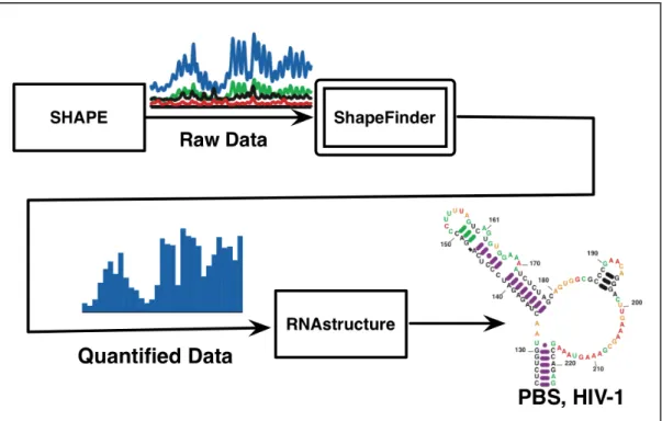
3.2 Introduction

(62)

as shown in Figure 3.1. SHAPE, as described in Chapter 2, is a chemical

modification technique which targets all four nucleotide types of an RNA to identify paired and unpaired regions [7, 8, 27]. The output of a SHAPE experiment is a spectrogram collected from DNA sequencing equipment [6]. A signal processing software suite, ShapeFinder (described in Chapter 2), was developed to process the SHAPE spectra in order to identify and quantify per nucleotide reactivity information [9, 10]_{. The per nucleotide reactivity data is used as a pseudo-free energy constraint}

in secondary structure prediction algorithms such as RNAstructure [45, 46]. From this, more accurate RNA structures are produced, in a high-throughput manner[6].

Figure 3.1. Block diagram of steps involved in determining RNA secondary structure using SHAPE. The output of SHAPE is a spectrogram whose signal is then

(63)

Before quantifying per nucleotide flexibility information, the ShapeFinder algorithm aligns the experiment to the known RNA sequence being analyzed. This step is necessary to ensure that the correct SHAPE modification is attributed to the correct nucleotide. First, the algorithm identifies the experimental sequence. The algorithm then attempts to match the experimental sequence to the RNA sequence by finding the position with the most matching nucleotides. If the experimental sequence has been incorrectly identified by mis-identifying, overlooking or including extra nucleotides, the matching algorithm will incorrectly align the sequences. A manual editing step is then required by the experimenter to manually align the experiment to the RNA sequence.