QUANTUM DYNAMICS OF EXCITED CHARGE CARRIER AT HETEROGENEOUS INTERFACE BETWEEN SEMICONDUCTOR AND ORGANIC MOLECULE
Lesheng Li
A dissertation submitted to the faculty at the University of North Carolina at Chapel Hill in partial fulfillment of the requirements for the degree of Doctor of Philosophy in the
Department of Chemistry.
Chapel Hill 2018
© 2018 Lesheng Li
ABSTRACT
Lesheng Li: Quantum Dynamics of Excited Charge Carrier at Heterogeneous Interface between Semiconductor and Organic Molecule
(Under the direction of Yosuke Kanai)
Developing a quantitative understanding of excited charge carrier dynamics at heterogeneous interfaces between semiconductor and organic molecules is of great practical importance in advanced technologically important applications. Despite great advances in this field, there remain many aspects that are yet to be understood such as the density of charge carrier, the role of defects, and the interactions with surface ligand. To this end, we aim to develop and apply a quantitative formulation based on first-principles quantum theory to elucidate how excited carrier dynamics at semiconductor-molecule interfaces depend on the atomistic details.
We then investigated how molecular details such as surface coverage and adsorbate species influence hot electron transfer. Counterintuitively, increasing surface coverage was found to suppress hot electron transfer probability because the increased delocalization of the hot electron accepting molecular states change the nonadiabatic couplings at the interface. In addition, the adsorbate species itself is an important factor in hot electron transfer not simply because of energy level alignments, but because the transfer is quite sensitive to nonadiabatic couplings.
ACKNOWLEDGEMENTS
I would first like to thank my parents, Yujiao and Anlin, for their continued support, encourage, and advice. Their guidance and whole-hearted love navigated me through numerous murky waters and ambiguous paths. I would also like to thank Jingwen who helped me in more ways than she will ever understand. Her constant support and open heart helped me through this adventure at just the right moments. I also want to acknowledge my best friends Yuanyuan Huo and Chao Wang, with whom I shared many moments with. Those moments witness our sincere friendship that keep the way it is.
I would also like to thank my advisor and most importantly, my mentor in all ways, Professor Yosuke Kanai for all of his help and support during my stay at Chapel Hill. His expertise, enthusiasm, and belief in my work allowed my research to extend far beyond what I had ever envisioned. His kindness and the countless lessons he taught me not only lead me to a qualified PhD, but also showed me the path to become a scientist.
TABLE OF CONTENTS
LIST OF TABLES ... x
LIST OF FIGURES ... xi
LIST OF ABBREVIATIONS ... xvi
CHAPTER 1: INTRODUCTION ... 1
CHAPTER 2: THEORETICAL AND NUMERICAL METHODS ... 13
2.1 Fewest-Switches Surface Hopping ... 14
2.1.1 Nonadiabatic couplings ... 16
2.1.2 Single-particle energies ... 17
2.2 Density Functional Theory and the Kohn-Sham Picture ... 18
2.3 First-Principles Molecular Dynamics ... 21
2.4 Many-Body Perturbation Theory ... 22
2.4.1 Many-body correction and quasi-particle description from GW calculations ... 22
2.4.2 One-particle Green’s function... 23
2.4.3 Lehmann representation of the one-particle Green’s function ... 25
2.4.4 Equation of motion for one-particle Green’s function ... 28
2.4.5 Hartree and Hartree-Fock approximation ... 29
2.4.6 Self-energy operator... 32
2.4.7 Dyson’s equation and quasi-particle equation ... 33
2.5 Procedure for Simulating Hot Carrier Dynamics... 39
CHAPTER 3: EXCITED ELECTRON DYNAMICS AT SEMICONDUCTOR- MOLECULE TYPE-II HETEROJUNCTION INTERFACES ... 40
3.1 Introduction ... 40
3.2 Computational Details and Interface Models ... 42
3.2.1 Computational details ... 42
3.2.2 Error introduced by classical-path approximation ... 44
3.2.3 Time step in FPMD simulation and nonadiabatic coupling calculations ... 48
3.2.4 On time dependence of many-body corrections ... 48
3.2.5 Convergence tests of the G0W0 calculation ... 49
3.2.6 Convergence of hot electron dynamics with respect to nuclear trajectory ensemble ... 52
3.2.7 Interface models ... 53
3.3 Results and Discussion ... 55
3.4 Summary ... 62
CHAPTER 4: DEPENDENCE OF HOT ELECTRON TRANSFER ON SURFACE COVERAGE AND ADSORBATE SPECIES AT SEMICONDUCTOR-MOLECULE HYBRID INTERFACES ... 63
4.1 Introduction ... 63
4.2 Computational Details and Interface Models ... 64
4.2.1 Computational details ... 64
4.2.2 Interface models ... 67
4.3 Results and Discussion ... 69
4.4 Summary ... 79 CHAPTER 5: EXAMINING THE EFFECT OF EXCHANGE-CORRELATION
INTERFACIAL CHARGE TRANSFER ... 81
5.1 Introduction ... 81
5.2 Computational Details and Interface Model ... 83
5.3 Results and Discussion ... 85
5.3.1 Energy level alignments and atomic trajectory ... 85
5.3.2 Nonadiabatic couplings ... 88
5.3.3 Interfacial charge transfer dynamics ... 91
5.4 Summary ... 95
CHAPTER 6: CONCLUSIONS ... 98
APPENDIX A: DERIVATION OF THE EQUATION OF MOTION OF THE SINGLE-PARTICLE GREEN’S FUNCTION ... 103
APPENDIX B: DERIVATION OF THE QUASI-PARTICLE EQUATION ... 108
APPENDIX C: DERIVATION OF THE HEDIN’S EQUATIONS... 109
C.1 Screened Coulomb Potential W ... 111
C.2 Self-energy Σ ... 112
C.3 Irreducible Polarizability P... 113
C.4 Vertex Function Γ ... 115
LIST OF TABLES
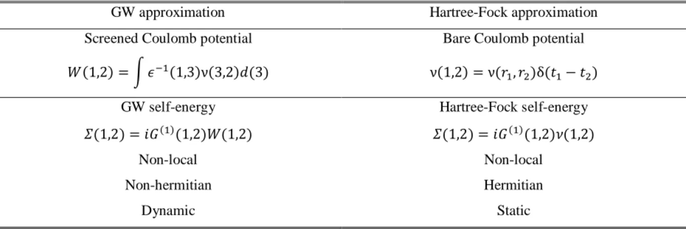
Table 2.1 | Comparison of the GW and Hartree-Fock approximations... 37 Table 3.1 | Monodentate: Standard deviation on atomic positions of the chemisorbed
cyanidin molecule in FPMD simulations of the interface structure, and displacements of atomic positions of an isolated cyanidin molecule induced by having an extra electron in a specific molecular state that corresponds to #87 in the interface case... 45
Table 3.2 | Bidentate: Standard deviation on atomic positions of the chemisorbed cyanidin molecule in FPMD simulations of the interface structure, and displacements of atomic positions of an isolated cyanidin molecule induced by having an extra electron in a
specific molecular state that corresponds to #88 in the interface case. ... 46
Table 4.1 | Peak probability and residence time of hot electron within the adsorbed
molecule at the interfaces. ... 71
Table 5.1 | Interfacial charge transfer time constant τ calculated by fitting the population
LIST OF FIGURES
Figure 1.1 | Schematic representation of hot carrier relaxation within the manifold of
semiconductor conduction/valence band electronic states. ... 1
Figure 1.2 | Schematic and band diagram of an ideal hot carrier solar cell. ... 2
Figure 1.3 | Schematic diagram of hot carrier dynamics in the context of QD-LEDs and how it could affect the performance of QD-LEDs. ... 3
Figure 1.4 | Demonstration of the electronic energy level alignments at a typical semiconductor-molecule interface and how hot carrier processes could take place at such a heterogeneous interface. ... 5
Figure 2.1 | Interpretation of the one-particle Green’s function. ... 24
Figure 2.2 | Direct term and exchange term in the interacting part of the EOM for one-particle Green’s function. ... 30
Figure 2.3 | Interpretation of the exchange term in the interacting part of the EOM for one-particle Green’s function. ... 32
Figure 2.4 | Feynman diagram interpretation of the first-order Dyson’s equation. ... 34
Figure 2.5 | Illustration of Hedin’s equations (left) and the GW approximation (right). ... 36
Figure 2.6 | Workflow of the numerical simulation for hot carrier dynamics. ... 38
Figure 3.1 | Maximum nonadiabatic couplings (NACs) of the cyanidin LUMO at H-Si(111):cyanidin interface during the FPMD simulations. Sharp peaks in the NACs are well captured with sufficient resolution with the time step of 0.48 fs used in the simulations. ... 47
Figure 3.2 | Many-body corrections (MBCs) for the equilibrium structure and a dynamical structure from the FPMD simulation (at t=500.16 fs). The diagonal line represents the equality of MBCs for the two structures. ... 49
Figure 3.3 | Convergence tests on different parameters for G0W0 calculations. The convergence of VBM-CBM energy gap, as a representative energy difference, is shown with respect to the parameters. ... 50
Figure 3.5 | Side and top views of the surface slab models with 144-Si-atom,
216-Si-atom, and 256-Si-atom (supercell). The bottom three layers were held fixed in
bulk positions. ... 52
Figure 3.6 | Spatial-resolved DOS for the conduction band states of the surface slab models with 144-Si-atom (on the left), 216-Si-atom (in the middle), and 256-Si-atom (on the right). The spatial-resolved DOS is calculated by averaging electron density in
the surface plane, and the silicon surface CBM is set to 0 eV as the reference energy. ... 53
Figure 3.7 | Population change for the excited electron using (a) 144-Si-atom, (b) 216-Si-atom, and (c) 256-Si-atom H-Si(111) surface slab models. (d) Time evolution of the averaged energy of the excited electron for the 144-Si-atom (red),
216-Si-atom (green), and 256-Si-atom (blue) H-Si(111) surface slab models. ... 54
Figure 3.8 | Interface structures of the H-Si(111):cyanidin interface in (a) monodentate and (b) bidentate adsorption modes, isosurface of the single-particle Kohn-Sham electronic wave function for the molecule’s LUMO is also shown at top. The spatial-resolved density of states (DOS) for the conduction band states of the (c) monodentate and (d) bidentate adsorption modes. The spatial-resolved DOS is calculated by averaging electron density in the surface plane, and the silicon surface
CBM is set to 0 eV as the reference energy. ... 56
Figure 3.9 | Population change for the excited electron in (a) monodentate and
(b) bidentate H-Si(111):cyanidin interface. Cyanidin’s LUMO is located energetically
below the surface CBM (E=0 eV) for both adsorption modes. ... 57
Figure 3.10 | Top: isosurface of the single-particle Kohn-Sham electronic wave function for the molecular state 87 (monodentate) and 88 (bidentate). Bottom: population change in the molecular state 87 (monodentate), state 88 (bidentate), and cyanidin LUMO. ... 57
Figure 3.11 | Time-averaged nonadiabatic couplings (NACs) matrix of the unoccupied states (in atomic units) for (a) monodentate and (b) bidentate adsorption modes. The NACs for the cyanidin LUMO and molecular state 87/88 are shown for comparison in (c) monodentate and (d) bidentate. The state index of the cyanidin LUMO is set to 1 as
the reference. NACs are particularly large close to the diagonal line. ... 58
Figure 3.12 | Population change in the cyanidin LUMO (blue), silicon states within 10 kBT above the surface CBM (red), and their sub-total (black) in the (a) monodentate and
(b) bidentate adsorption modes. ... 59
Figure 3.13 | (a) Isosurface of the defect electronic state that is induced by having a
missing hydrogen atom at the surface. Population evolution of the electronic states within 10 kBT above the surface CBM (red) and of the defect electronic state (blue) (b) when the defect state is located 1.10 eV below the surface CBM and (c) when the defect state is
Figure 4.1 | Top view of the simulation cells for the H-Si:C, H-Si:2C, H-Si:A, and H-Si:2A interfaces. The H-Si(111) surface was modeled using a 144-Si-atom slab with
eight layers. ... 67
Figure 4.2 | Side view of the interface models investigated in this work. ... 68 Figure 4.3 | Spatial-resolved density of states for (a) H-Si:C, (b) H-Si:2C, (c) H-Si:A, and
(d) H-Si:2A interfaces, where the DOS is calculated by averaging the electron density in the surface plane. Hot electron states are indicated by arrows and the surface CBM
is set as the reference energy of 0 eV in the spatial-resolved DOS figures. ... 69
Figure 4.4 | Probability of locating the excited electron at a specific energy as a function of time at the interfaces of (a) H-Si:C, (b) H-Si:2C, (c) H-Si:A, and (d) H-Si:2A. The reference energy of 0 eV corresponds to the surface CBM. The hot electron accepting state that dominantly localized on the molecule is referred to as hot electron state. The excited electron was initially populated in a semiconductor state with energy of ~3.6 eV above the surface CBM as indicated by P(t=0). ... 70
Figure 4.5 | Ensemble averaged energy for the excited electron at the interfaces. ... 71
Figure 4.6 | (a) Probability change and (b) isosurface of the single-particle Kohn-Sham electronic wave function of the hot electron states at the interfaces. Hot electron states
become delocalized over both molecules when the surface coverage is increased. ... 72
Figure 4.7 | Peak probability of the hot electron within the unoccupied electronic states as a function of state index based on time-averaged energy, together with the wave function contribution from the adsorbate for each unoccupied electronic state. Red triangle marker represents the pure molecular state with the largest hot electron
probability and is referred to as hot electron state. ... 73
Figure 4.8 | Isosurface of the single-particle Kohn-Sham electronic wave function of the molecular states for (a) isolated two Cyanidin molecules, (b) the interface between Cyanidin molecules and the H-Si(111) surface with a separation distance of 1 angstrom. The geometry of the Cyanidin molecules was taken directly from the H-Si:C interface,
where the bottom two oxygen atoms were terminated by hydrogen atoms. ... 75
Figure 4.9 | NACs (in a.u.) between the hot electron state and the unoccupied
semiconductor states at the four interfaces of (a) H-Si:C, (b) H-Si:2C, (c) H-Si:A, and (d) H-Si:2A. The positions of the hot electron states are labeled out in the matrix by
dash lines... 76
Figure 4.10 | Density of nonadiabatic coupling (NAC) as a function of NAC magnitude (in a.u.) between the hot electron state and higher-lying/lower-lying semiconductor states for the (a) Cyanidin and (b) Alizarin cases. Y-axis is shown in log scale. Bin size
Figure 4.11 | Density of NAC as a function of NAC magnitude between the hot electron state and the lower-lying semiconductor states at the H-Si:C (blue) and H-Si:A (red)
interfaces. Bin size of 5×10⁻⁴ was used for the Gaussian broadening where 2=5×10⁻⁷. ... 78
Figure 4.12 | Probability change of the hot electron state for the interfaces of
H-Si:C (blue), H-Si:A (red), and H-Si:Ashift (dashed black). H-Si:Ashift represents the case where the hot electron state was artificially shifted away to the same energy of
the H-Si:C interface. ... 79
Figure 5.1 | Top and side view of the 3×3 super cell used in our calculations. Pink, blue,
and cyan spheres represent B, N, and Li atoms, respectively. ... 83
Figure 5.2 | Convergence tests of the parameters of (a) contour grid size (grid size), (b) projective dielectric eigenpotential basis vectors (NPDEP), and (c) Lanczos steps
(NLanczos) used in the G0W0 calculations with respect to the energy gap. ... 84
Figure 5.3 | Atom-projected density of states (PDOS) calculated using (a) PBE and (b) PBE0 XC approximations. The lowest unoccupied electronic state (Li state) is set
to 0 as the reference energy. ... 86
Figure 5.4 | (a) The normalized distribution of the normal distance between the Li ion and the BN sheet in FPMD simulations with PBE (red) and PBE0 (blue) XC
approximations. The normalized distribution of the KS eigenvalues in FPMD simulations with PBE (red) and PBE0 (blue) XC approximations, for (b) Li state, (c) BN-1 state, and (d) BN-2 state. The eigenvalue of the Li state at the equilibrium
structure is set to 0 as the reference energy for the eigenvalue distribution figures. ... 87
Figure 5.5 | Time-averaged nonadiabatic (NAC) matrices for unoccupied electronic states. State indices of 1, 2, and 3 represent the Li state (the lowest unoccupied electronic state), BN-1 state, and BN-2 state, respectively. NAC calculated from PBE and PBE0
approximations are shown in the upper-triangle and lower-triangle of (a). NAC calculated from PBEPBE0 (NAC calculated with PBE functional using the FPMD trajectories based on the forces from the PBE0 functional) and PBE0PBE (NAC calculated with PBE0 functional using the FPMD trajectories based on the forces from the PBE functional) are shown in the upper-triangle and lower-triangle of (b). Time-averaged NAC values between the Li state (index of 1) and BN states (index of 2 and 3) computed from PBE, PBE0, PBEPBE0, and PBE0PBE calculations are summarized in (c). Ratio of the NAC magnitudes between PBE and PBE0
calculations (NACPBE: NACPBE0) is shown in (d). ... 89
Figure 5.6 | Red symbols show many-body corrections (MBCs) for the equilibrium structure (at t=0 ps) and the dynamical structures that are taken from the FPMD simulations at evenly spaced time intervals (at t=2, 4, 6, and 8 ps). The averaged MBCs (black dashed line) and the standard deviation (blue box) for the electronic
Figure 5.7 | Time-averaged energy levels from the FPMD simulation of the Li state (blue), BN-1 state (red), and BN-2 state (green) according to PBE, PBE0, G0W0@PBE, and G0W0@PBE0 calculations. The Li state is set to zero as the reference energy. ... 94
Figure 5.8 | Population change of the Li state calculated from the different ε: NAC
combinations. Fitting the population change of the Li state to the two-state model given by Eq. 5.2 yields the time constant of the interfacial charge transfer as 0.37, 1.05, 1.74, and 2.40 ps for εPBE: NACPBE, εG0W0@PBE: NACPBE, εPBE0: NACPBE0,
LIST OF ABBREVIATIONS
BET Back-electron transfer
BO Born-Oppenheimer
CBM Conduction band minimum CPA Classical-path approximation DFT Density functional theory DOS Density of states
DSSC Dye-sensitized solar cell EA Electron affinity
EOM Equation of motion ET Electron transfer FFT Fast Fourier transform
FPMD First-principles molecular dynamics FSSH Fewest-switches surface hopping GGA Generalized gradient approximation G0W0 One-shot GW calculation
HET Hot electron transfer
HF Hartree-Fock
HOMO Highest occupied molecular orbital
IE Ionization energy, same as ionization potential IET Interfacial electron transfer
IP Ionization potential, same as ionization energy
KS-DFT Kohn-Sham Density functional theory LHS Left-hand side
LUMO Lowest unoccupied molecular orbital MBC Many-body correction
MBPT Many-body perturbation theory
MD Molecular dynamics
NA Nonadiabatic
NAC Nonadiabatic coupling
NAMD Nonadiabatic molecular dynamics PBE Perdew-Burke-Erzerhof
PBE0 Perdew-Burke-Erzerhof with 0.25 Hartree-Fock exchange PDOS Projected density of states
PES Potential energy surface PPA Plasmon-pole approximation
QD Quantum dot
QP Quasi-particle
RHS Right-hand side
RPA Random-phase approximation sc-GW Self-consistent GW
CHAPTER 1: INTRODUCTION
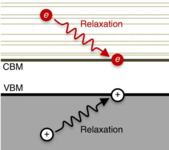
When a photon with energy ℏ𝜔 ≥ 𝐸𝑔 is first adsorbed by a semiconductor (with an energy band gap of 𝐸𝑔), the immediate aftermath is the photogeneration of an electron-hole pair.1 In the single-particle description of quantum mechanics, excited electrons with excess energy above the conduction band minimum (CBM) of a material are called hot electrons.1-2 Similarly, excited holes with energy below the valence band maximum (VBM) are called hot holes. The term hot carrier
refers to the fact that prior to any scattering with lattice phonons, the photoexcited electron/hole has energy in excess of the fundamental band gap and thus is considered to be hot. Hot carriers lose their excess energy by relaxation within the manifold of the conduction/valence band electronic states through coupling with lattice phonons (i.e. atomic vibrations) to the band edges (VBM or CBM) as shown schematically in Figure 1.1.
This hot carrier relaxation process is of great practical importance in various optical and electronic device technologies3-11 including solar energy conversion10,12-13 and light emitting diodes (LEDs).2,14-17 Also, it is a scientifically intriguing process in regard to the underlying physics associated with the coupling between the electronic and ionic degrees of freedom.
Figure 1.2 | Schematic and band diagram of an ideal hot carrier solar cell.
special class of solar cells, the idea was that one could take advantage of the photogenerated hot carriers (hot electrons and hot holes) before they have enough time to relax to the band edges (VBM for hot holes and CBM for hot electrons).1,12 Thus, the practical realization of the concept for HCSC ultimately relies on finding a way to increase the relaxation time of the hot carriers so that they can be efficiently collected via the selective energy contact (SEC) to do work before losing their excess energy.12,18
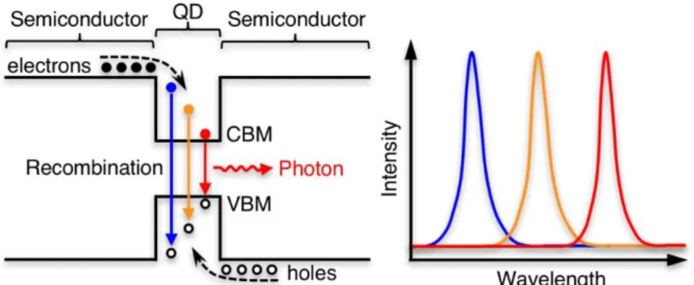
Figure 1.3 | Schematic diagram of hot carrier dynamics in the context of QD-LEDs and how it could affect the performance of QD-LEDs.
importance for QD-LEDs2,19 in order that the excess energy of hot carriers can be transferred efficiently to photons instead of being wasted by phonons as illustrated in Figure 1.3.
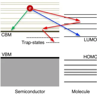
Figure 1.4 | Demonstration of the electronic energy level alignments at a typical semiconductor-molecule interface and how hot carrier processes could take place at such a heterogeneous interface.
that are specific to distinctive dynamical processes is still challenging. This is because several dynamical processes with similar time scales46 are operating simultaneously at the heterogeneous interfaces42-43 during hot carrier relaxation, as illustrated in Figure 1.4.
These dynamical processes can occur in parallel, they compete with each other and ultimately determine the efficiency of the devices. Most importantly, the interplay among these kinetic processes that hot carriers can undergo significantly obfuscate the details of hot carrier dynamics.47-48 In spite of the enormous amount of effort that researchers have devoted to semiconductor-molecule interfaces, many details of hot carrier dynamics that occur at interfaces remain unknown and are inherently challenging to uncover.44 These difficulties originate from the fact that there exist two parts of interest involved in hot carrier dynamics at the semiconductor-molecule heterogeneous interfaces: (i) the semiconductor material and (ii) the surface semiconductor-molecules. The former is usually studied by solid-state physicists, while the latter is generally investigated by chemists.49 Both aspects of these heterogeneous interfaces have their own areas of scientific interest: organic molecules have discrete localized electronic states, unique vibrational spectra, and well-defined directional bonds. Semiconductor materials, on the other hand, have continuous bands of delocalized electronic and vibrational states, can be easily modified and doped, and contain numerous defects that disrupt regular bonding patterns. In addition, the electronic structure of the semiconductor material is also affected by its size, shape, and morphology.44 Realizing all of these difficulties, developing a comprehensive knowledge of the hot carrier dynamics in complex systems (such as heterogeneous interfaces between semiconductor material and organic molecules) calls for accurate modeling of excited carrier dynamics at the atomic level.
heterogeneous interfaces depend on the atomistic details, such as the molecular chemisorption, density of states (DOS) in the semiconductor conduction band, and the surface molecule. As we have discussed above, unlike charge transfer from the molecule to the semiconductor surface or hot carrier relaxation in bulk semiconductors, several dynamical mechanisms are operating simultaneously at the semiconductor-molecule interfaces and their relative importance is at the heart of elucidating the hot carrier process thoroughly. We turn to first-principles quantum theory simulations because they are able to provide a unique perspective on the interfacial electron dynamics and most closely mimic the processes as they can occur in nature.44 First-principles simulation complements the simplified phenomenological models,50-56 which allow us to systematically investigate the influence of various interface characteristics of the hot carrier dynamics by varying model parameters. The atomistic simulation treats the interfaces in full, realistic detail, and describes the evolving geometric and electronic structure of the organic molecule, the semiconductor surface, and the electrolyte in real time. The ab initio treatment of the interfaces makes it possible to avoid fitting parameters and to build the theory starting from the fundamental laws of physics.
semiconductor-molecule heterogeneous interfaces from several aspects via first-principles quantum mechanics simulations.
First, we employ first-principles electron dynamics simulations to investigate how the molecular details influence the quantum dynamics of excited electrons at the semiconductor-molecule type-II heterojunctions. A representative interface between the hydrogen-terminated silicon (111) surface and a dye molecule cyanidin was investigated here because silicon, being the foundation of modern electronic devices, has been studied extensively in the past decade,57-59 and continues to draw attention.60 As we have discussed previously, the transfer of the injected electron back to the oxidized molecule (or to the electrolyte molecule) is of great concern in DSSCs because the transfer negatively impacts device performance.42,44-45 This so-called back-electron transfer (BET) is often described using an effective two-state model, symbolically denoted as 𝑆𝑒𝑚𝑖𝑐𝑜𝑛𝑑𝑢𝑐𝑡𝑜𝑟(𝑒−) − 𝑀𝑜𝑙𝑒𝑐𝑢𝑙𝑒+→ 𝑆𝑒𝑚𝑖𝑐𝑜𝑛𝑑𝑢𝑐𝑡𝑜𝑟 − 𝑀𝑜𝑙𝑒𝑐𝑢𝑙𝑒 . With TiO2 as the
adsorbed molecule at a typical semiconductor-molecule interface. Using first-principles dynamics simulations, we show that the electron transfer can be quite fast when no defects are present to trap the hot electron at the semiconductor surface. Hot electron transfer to the chemisorbed molecule was observed but was short-lived on the molecule. Interfacial electron transfer to the chemisorbed molecule was found to be largely decoupled from hot electron relaxation within the semiconductor surface. While the hot electron relaxation was found to take place on a time scale of several hundred femtoseconds, the subsequent interfacial electron transfer was slower by an order of magnitude. At the same time, this secondary process of picosecond electron transfer is comparable in time scale to typical electron trapping into defect states in the energy gap. Contrary to popular belief, hot electron transfer is not the mechanism responsible for the ultra-fast electron transfer to the adsorbed molecule. This work is the subject of the paper published in The Journal of Physical Chemistry Letters2016, 7, 1495.30
first-principles quantum dynamics simulation of excited electrons, the HET process from semiconductor to adsorbed molecule was indeed observed.30 This provided us with an atomistic model that we can use to study how the HET dynamics can be tuned at the atomistic level. Following this work, we went further to investigate whether or not one could manipulate the hot electron transfer process at semiconductor-molecule heterogeneous interfaces by tuning the molecular details such as surface coverage and adsorbate species. Counterintuitively, increasing surface coverage does not enhance the HET probability, but significantly suppress such a dynamical process. This is because the increased delocalization of the hot electron accepting molecular states change the nonadiabatic couplings at the interface. In addition, adsorbate species itself is an important factor in HET process not simply because of energy level alignments, but because the transfer is quite sensitive to the nonadiabatic couplings. Our work shows that controlling of nonadiabatic couplings at the molecular level, not only the energy level alignments as often assumed, is an essential factor in developing a “design principle” for enhancing hot electron transfer. This work is the subject of the paper recently submitted to Physical Chemistry Chemical Physics.
magnitude consistency for the charge transfer rate is encouraging even for this rather extreme model of heterojunction interface, continued advancement in electronic structure methods is required for quantitatively accurate determination of the transfer rate. This work is the subject of the paper published in Journal of Chemical Theory and Computation2017, 13, 2634.
The remaining dissertation is organized as follows. CHAPTER 2 provides a background to the computational methods used throughout the dissertation, including fewest-switches surface hopping, density functional theory and Kohn-Sham picture, first-principles molecular dynamics, many-body perturbation theory with GW approximation, and the workflow for numerical simulation of hot carrier dynamics. CHAPTER 3 discusses the excited electron dynamics at a representative semiconductor-molecule type-II interfaces. CHAPTER 4 provides the discussion on
CHAPTER 2: THEORETICAL AND NUMERICAL METHODS
Hot charge carrier dynamics at semiconductor-molecule heterogeneous interfaces depend ultimately on several factors, such as the energy level alignments and the extent of quantum mechanical coupling between the electronic structures of the semiconductor material and the molecule. Therefore, developing a comprehensive knowledge of hot carrier processes calls for accurate modeling of excited electron dynamics at the atomistic level because impartial interpretation of spectroscopic measurements is challenging when various dynamical processes operate with similar time scales simultaneously at the interfaces.46 To this end, nonadiabatic molecular dynamics (NAMD)43,46,79-81 has become quite popular in recent years for investigating hot carrier dynamics at semiconductor-molecule interfaces.30,43,75,82-84 While significant advancement has been made in simulating hot carrier dynamics from first-principles theory (no empirical parameters from experiments are employed) in the past few years,43,75,82-87 such as using the fewest-switches surface hopping approach as described in the following section, the approach currently suffers from the practical limitation of having inaccurate description of interfacial electronic structure. In particular, the use of Kohn-Sham density functional theory (KS-DFT) is problematic for describing the energy level alignments at the heterogeneous interfaces in practice.88-89
(1) Efficient calculation of nonadiabatic couplings, which describe the coupling of electrons to atomic vibrations, within first-principles molecular dynamics simulations.
(2) Incorporation of many-body interaction in the single-particle picture of independent electrons (i.e. quasi-particle description) through solving the Dyson’s equation using many-body perturbation theory.
2.1 Fewest-Switches Surface Hopping
unphysical dynamics outside of the electronic crossings.90 Later in 1990, Tully proposed an algorithm which minimizes the number of state switches, subject to maintaining the correct statistical distribution of state populations at all times.46 Such an algorithm is therefore named as switches surface hopping” (FSSH). Compared to the original TSH algorithm, the “fewest-switches” criterion is derived specifically to limit the electronic hops to the region of electronic crossings (i.e. with strong nonadiabatic couplings).
The FSSH approach44,46,61,76 was further extended into a formulation based on the single-particle description within the so-called classical-path approximation (CPA) as formulated by Prezhdo and co-workers.43-44 Here, instead of using many-body adiabatic states as in Tully’s original surface hopping method, Prezhdo proposed the employment of single-particle wave functions as the states where the hops could take place. In addition, the CPA assumes a classical equilibrium path that is representative of the system’s nuclei at all times and surface hops do not significantly influence the nuclear dynamics.
Within the single-particle FSSH approach, the instantaneous probability for an electron transition (hop) from state 𝑘 to state 𝑗 in time ∆𝑡 is governed by
𝑔𝑘𝑗(𝑡) = {2ℏℑ𝑚(𝜌𝑘𝑗𝐻𝑗𝑘) − 2ℜ𝑒(𝜌𝑘𝑗𝐷𝑗𝑘)} ∆𝑡/𝜌𝑘𝑘(𝑡) (2.1)
where 𝜌 is the density matrix for the excited electron, 𝐷 is the nonadiabatic coupling (NAC) matrix, and 𝐻 is the single-particle Hamiltonian matrix for the excited electron. The probability for a stochastic hop from state 𝑘 to state 𝑗 is given by
𝐵𝑘→𝑗(𝑡) = {exp (−
𝜀𝑗− 𝜀𝑘
𝑘𝐵𝑇 ) 𝑖𝑓 𝜀𝑗 ≥ 𝜀𝑘
1 𝑖𝑓 𝜀𝑗 ≤ 𝜀𝑘 (2.3) where 𝜀𝑘,𝑗 are the single-particle energies for satisfying detailed balance.
The density matrix for an excited electron can be set up with density operator
𝜌̂(𝑡) = |𝜙(𝑡)⟩⟨𝜙(𝑡)| (2.4)
where 𝜙 is the wave function of the excited electron. We can then obtain the time-evolution of the density matrix element by using the Liouville-von Neumann equation91
𝑖ℏ 𝑑
𝑑𝑡𝜌 = [𝐻, 𝜌] − 𝑖ℏ[𝐷, 𝜌]. (2.5)
The second term on the right-hand side arises because the electronic state depends on the (time-dependent) positions of classical nuclei. In the adiabatic basis, the time evolution of the density matrix element can be written as
𝑖ℏ𝜌̇𝑖𝑗 = ∑[(𝜀𝑙𝛿𝑖𝑙− 𝑖ℏ𝐷𝑖𝑙)𝜌𝑙𝑗 − 𝜌𝑖𝑙(𝜀𝑙𝛿𝑙𝑗 − 𝑖ℏ𝐷𝑙𝑗)]
𝑖
(2.6) where 𝜀𝑙 is the single-particle energies of state 𝑙, and 𝐷𝑖𝑙 is the NAC matrix element between state 𝑖 and state 𝑙. As shown in EQUATION 2.6, NACs and single-particle energies are the two essential ingredients in this approach, and they can be obtained from first-principles quantum mechanical calculations as follows.
2.1.1 Nonadiabatic couplings The NACs can be expressed as
𝐷𝑖𝑗 = ⟨𝜓𝑖(𝑅(𝑡))| 𝜕𝜕𝑡 |𝜓𝑗(𝑅(𝑡))⟩
= ⟨𝜓𝑖(𝑅(𝑡))|𝛻𝑅|𝜓𝑗(𝑅(𝑡))⟩ ∙
𝑑𝑅 𝑑𝑡
=⟨𝜓𝑖(𝑅(𝑡))|𝛻𝑅𝐻̂|𝜓𝑗(𝑅(𝑡))⟩ 𝜀𝑗(𝑅(𝑡)) − 𝜀𝑖(𝑅(𝑡)) ∙
𝑑𝑅 𝑑𝑡
where 𝐷𝑖𝑗 is the NAC between two states 𝑖 and 𝑗, 𝜓𝑖(𝑅(𝑡)) and 𝜀𝑖(𝑅(𝑡)) are the single-particle
eigenfunction and eigenvalue for state 𝑖 at the nuclear coordinate 𝑅(𝑡), and 𝐻 is the Kohn-Sham (KS) Hamiltonian. We implemented the numerical calculation of NACs using the time-derivative by enforcing the phase continuity as described in refs 30,92-93. The NACs can be calculated efficiently on-the-fly within the first-principles molecular dynamics (FPMD) simulations. We follow the prescription by Hammes-Schiffer and Tully for calculating the NACs numerically, from KS adiabatic wave functions at adjacent time steps.76 In practice, the NACs are calculated at discrete time steps, and accurate sampling is crucial because NAC becomes significant rather infrequently for heterogeneous systems such as semiconductor-molecule interfaces. Inadequate sampling of NAC therefore could qualitatively impact the electron dynamics. The on-the-fly
calculations in FPMD simulations allow us to obtain accurately sample NACs efficiently even for very large systems containing a few thousand electrons.
2.1.2 Single-particle energies
Single-particle energy level alignments at semiconductor-molecule interfaces were modeled using quasi-particle (QP) energies within the G0W0 approximation (details will be discussed in
SECTION 2.3). QP energies were obtained from
𝜀𝑖𝑄𝑃(𝑡) = 𝜀𝑖𝐾𝑆(𝑡) + [1 − ⟨𝜓
𝑖(𝑡)|𝜕Σ(𝜔)𝜕𝜔 | 𝜔=𝜀𝑖
|𝜓𝑖(𝑡)⟩]
−1
∙ ⟨𝜓𝑖(𝑡)|Σ(𝑟, 𝑟′; 𝜀
𝑖) − 𝜈𝑋𝐶(𝑟)𝛿(𝑟 − 𝑟′)|𝜓𝑖(𝑡)⟩
(2.8)
KS wave functions 𝜓𝑖(𝑡) at time 𝑡. Because of the very high computational cost associated, even within the G0W0 approximation, it is computationally impractical to take into account the time-dependence of the QP energies. Instead, we obtain the many-body corrections on top of KS energies at the equilibrium geometry, and we apply the same (time-independent) many-body corrections to correct individual time-dependent KS energies to obtain the time-dependent QP energies along the atomic trajectory, i.e. ∆𝜖𝑖(𝑡) = 𝜀𝑖𝐾𝑆(𝑡) + ∆𝜖
𝑖(𝑡 = 0). We have examined the
validity of this approximation for different interfaces as discussed in each chapter.
2.2 Density Functional Theory and the Kohn-Sham Picture
By using density functional theory (DFT), one can determine the electronic ground state and energy exactly, provided that the universal density functional 𝐹(𝜌) is known. The problem at present is practical rather than conceptual, because of the inherent difficulty in solving the full many-body problem. The main difficulty is that electrons interact among themselves via Coulomb two-body forces. As a consequence, the presence of an electron in one region of space influences the behavior of other electrons in other regions, so they cannot be considered as individual entities. This is called the quantum many-body problem. A convenient strategy is to separate the classical electrostatic energy (Hartree term) from the quantum mechanical exchange and correlation energy contributions.94 Therefore, the energy of a many-body electronic system can be written in the following way:
𝐸 = 𝑇 + 𝑉𝑒𝑥𝑡+1 2∫
𝜌(𝑟)𝜌′(𝑟′)
|𝑟 − 𝑟′| 𝑑𝑟𝑑𝑟′ + 𝐸𝑥𝑐 (2.9)
𝐸𝑥𝑐 =1 2∫
𝜌(𝑟)𝜌(𝑟′)
|𝑟 − 𝑟′| [𝑔(𝑟, 𝑟′) − 1]𝑑𝑟𝑑𝑟′ (2.10) where 𝑔(𝑟, 𝑟′) is the two-electron correlation function (which turns out to be the pair correlation
function of electrons95). Within the Kohn-Sham approach,96 a set of self-consistent independent-electron Schrödinger-like equations are solved to obtain the density and the total energy of the system, where an approximation for the exchange-correlation potential of the electrons is required for practical calculations. These equations are referred to as the Kohn-Sham (KS) equations:
𝐻̂𝐾𝑆𝜑𝑖𝐾𝑆(𝑟) = 𝜀𝑖𝐾𝑆𝜑𝑖𝐾𝑆(𝑟) (2.11)
where 𝜑𝑖𝐾𝑆(𝑟) are called KS orbitals, 𝜀
𝑖𝐾𝑆 are the eigenvalues of the KS orbitals, and 𝐻̂𝐾𝑆 is the
KS Hamiltonian which can be expressed in the following form: 𝐻̂𝐾𝑆 = −1
2∇2+ 𝜈𝑒𝑥𝑡(𝑟) + 𝜈ℎ(𝑟) + 𝜈𝑋𝐶(𝑟) (2.12) where the first term is the kinetic energy, 𝜈𝑒𝑥𝑡(𝑟) is the interaction with external field, 𝜈ℎ(𝑟) is the
Hartree term, and 𝜈𝑋𝐶(𝑟) is the exchange-correlation potential, which can be expressed as
𝜈𝑋𝐶(𝑟) = 𝛿𝐸𝑋𝐶(𝜌)
𝛿𝜌(𝑟) (2.13)
𝜌(𝑟) = 2 ∑|𝜑𝑖(𝑟)|2 𝑁𝑠
𝑖=1
(2.14)
where we have chosen the closed shell situation, with the occupation numbers 2 for 𝑖 ≤ 𝑁𝑠 and 0
for 𝑖 > 𝑁𝑠, with 𝑁𝑠 = 𝑁/2, the number of doubly occupied orbitals.
As we have discussed in previous section, the probability of a hop in the FSSH method assumes the accuracy of nonadiabatic couplings as well as energy level alignments as shown in EQUATION 2.6. In a system such as the interface between a molecule and a semiconductor surface, the energy level alignments are very important in order to accurately describe the kinetic processes such as hot carrier dynamics. However, the absolute values according to KS-DFT calculations often show large errors compared to experiments, leading to less accurate energy level alignments. Thus, KS-DFT calculations may not provide the energy level alignments that are accurate enough to perform further surface hopping calculations. Another approach is to use many-body perturbation theory (MBPT) with the GW approximation. The Green’s function represents the probability of observing an electron (or a hole) at position r, at time t given that there was an electron (a hole) at position r’ at time t’. In this sense, it constitutes a generalization of the static pair correlation function 𝑔(𝑟, 𝑟′)
2.3 First-Principles Molecular Dynamics
First-principles molecular dynamics (FPMD), also referred to as ab-initio molecular dynamics (AIMD), is an approach to simulate the same dynamics as classical MD, but instead of pre-defining the potentials used throughout the simulation, the forces acting on the nuclei are calculated on-the-fly during the simulation using electronic structure theory. In this section, we will assume that all the nuclei (together with their core electrons) can be treated as classical particles. And we only consider the systems for which a separation between the classical motion of the atoms and the quantum motion of the electrons can be achieved, i.e. under the Born-Oppenheimer (BO), or adiabatic, approximation. Such an assumption is regularly made and is generally valid for many chemical systems.
To be concise, the BO approximation assumes that the motion of the electrons is entirely decoupled from the motion of the nuclei, and they can therefore be separated. This is because the time scale associated with the motion of nuclei is usually much longer than that of the electrons. For any given ionic configuration, it is possible to calculate the self-consistent electronic ground state, and consequently the forces acting on the ions by using the Hellmann-Feynman theorem.97 The obtained ionic forces allow then to evolve the classical nuclei trajectories in time. Thus, the general approach of FPMD is to calculate the ground state electronic system based on a specific configuration of nuclei from a first-principles electronic structure calculation, and to advance the classical nuclei using Newton’s equation of motion where forces can be determined from the ground state electronic structure. The force acting on the nuclei can be expressed as
𝐹𝐼 = −∇𝐼𝐸𝐼 = −∇𝐼[⟨Ψ0|𝐻𝑒|Ψ0⟩] (2.15)
ground state KS orbital in the KS picture. Feynman showed that if the many-body wave function is an eigenfunction or a linear combination of eigenfunctions of the electronic Hamiltonian, 𝐻̂𝑒,
EQUATION 2.15 can be simplified to the following form98
𝑀𝐼𝑹̈𝐼 = −⟨Ψ0|∇𝐼𝐻̂𝑒|Ψ0⟩ (2.16)
where 𝑀𝐼 is the mass of the ion and 𝑹̈𝐼 is the acceleration of the nucleus. Within the description of KS-DFT, 𝐻̂𝑒 is the KS Hamiltonian and the forces can be determined for a specific nuclear configuration by evaluating the expression ∇𝐼𝐻̂𝑒𝐾𝑆. Therefore, a practical algorithm of FPMD could be summarized as follows:97
(1) Self-consistent solution of the KS equations for a given ionic configuration 𝑹𝐼; (2) Calculation of the forces acting on the ions via the Hellmann-Feynman theorem; (3) Integration of the Newton’s equations of motion for the nuclei;
(4) Update of the ionic configuration.
2.4 Many-Body Perturbation Theory
2.4.1 Many-body correction and quasi-particle description from GW calculations
In the context of quantum field theory, the quasi-particle energies describe the single-particle energies of the interacting excited electron/hole and they are accessible using the Green’s function formalism.99 By solving Dyson’s equation with the so-called GW approximation to the self-energy operator Σ in the context of many-body perturbation theory (MBPT), the quasi-particle (QP) energies can be obtained by applying the many-body corrections (MBCs) on top of the KS eigenvalues
𝜀𝑘𝑄𝑃 = 𝜀𝑘𝐾𝑆+⟨𝜓𝑘(𝑅(𝑡))|𝛴(𝜀) − 𝜈𝑋𝐶|𝜓𝑘(𝑅(𝑡))⟩
where the second term at the right-hand side is the MBC and vxc is the exchange-correlation potential in the KS Hamiltonian. Within GW approximation, self-energy operator Σ is obtained from the Green’s function (G) and the screened Coulomb interaction (W), and 𝑍 is the renormalization factor which is a derivative of the self-energy operator with respect to the energy.
2.4.2 One-particle Green’s function
One-particle Green’s function (also called as single-particle Green’s function)99 is an important concept in computing electronic excitations, involving both adding and removing one electron from the system. By using this concept, one is able to obtain a better fit to experimental data of photoemission or inverse photoemission. The time-ordered one-particle Green’s function is defined as
𝐺(1)(1,2) = −𝑖⟨𝛹
0𝑁|𝑇̂𝜓̂(1)𝜓̂†(2)|𝛹0𝑁⟩ (2.18)
where 1 ≡ (𝑟1, 𝑡1), and 2 ≡ (𝑟2, 𝑡2) are Hedin’s compact notations to indicate space coordinates r
and time t, and Ψ0𝑁 is the ground state many-body wave function of the system containing N
electrons, 𝑇̂ is the time-ordering operator, 𝜓̂(𝑟, 𝑡) and 𝜓̂†(𝑟, 𝑡) are field operators in the Heisenberg representation for annihilation and creation operators, which destroy or create an electron at position r and at time t. Atomic units (ℏ = 𝑚 = 𝑒 = 1) are used here. The time-ordering
operator 𝑇̂ has the following format
𝑇̂[𝐴(𝑥)𝐵(𝑦)] = {𝐴(𝑥)𝐵(𝑦) 𝑖𝑓 𝑥±𝐵(𝑦)𝐴(𝑥) 𝑖𝑓 𝑥0> 𝑦0
0 < 𝑦0 (2.19)
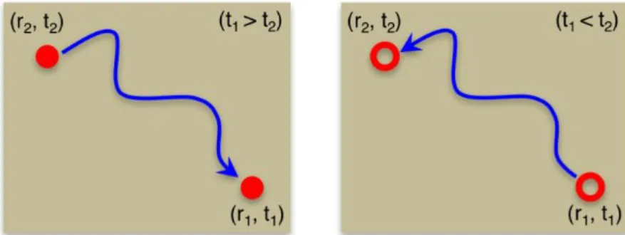
corresponding hole.100 Hence the Green’s function can be interpreted as a propagator of a state that involves adding or removing an electron or hole (as shown in Figure 2.1), which indicates that one can use the Green’s function to describe the electron affinities and ionization potentials, and to simulate photoemission or inverse photoemission experiments.
Figure 2.1 | Interpretation of the one-particle Green’s function.
If we assume that the Hamiltonian and field operator are not an explicit function of time, we can show that the time-ordered Green’s function will depend only on the time difference 𝜏 where 𝜏 = 𝑡1− 𝑡2, by using Schrödinger representation of the field operator
𝜓̂(1) = 𝑒𝑖𝐻̂𝑡𝜓̂(1)𝑒−𝑖𝐻̂𝑡 (2.20)
and the relation
𝐻̂|𝑁, 0⟩ = 𝐸𝑁,0|𝑁, 0⟩ (2.21)
where we used the short-hand notation of |𝑁, 0⟩ to represent the ground state many-body wave function of a system with 𝑁 electrons 𝛹0𝑁, we can represent the one-particle Green’s function as
𝐺(1)(𝑟
1, 𝑡1, 𝑟2, 𝑡2) = 𝐺(1)(𝑟1, 𝑟2; 𝜏)
= −𝑖𝑒𝑖𝐸𝑁,0𝜏⟨𝑁, 0|𝜓̂(𝑟
1)𝑒−𝑖𝐻̂𝜏𝜓̂†(𝑟2)|𝑁, 0⟩𝜃(𝜏)
+ 𝑖𝑒−𝑖𝐸𝑁,0𝜏⟨𝑁, 0|𝜓̂†(𝑟
2)𝑒𝑖𝐻̂𝜏𝜓̂(𝑟1)|𝑁, 0⟩𝜃(−𝜏)
EQUATION 2.22 is referred to as the Schrödinger representation of the one-particle Green’s function.
2.4.3 Lehmann representation of the one-particle Green’s function
In order to remove the time operators inside the expectation values of the Schrödinger representation of the one-particle Green’s function in EQUATION 2.22, we insert into the one-particle Green’s function a complete set of eigenstates of the system with 𝑀 particles, |𝑀, 𝑛⟩, where 𝑛 is a general label to describe the possible excited states for the system. Since the states form a complete set, we can write the closure relation
∑|𝑀, 𝑛⟩⟨𝑀, 𝑛|
𝑀,𝑛
= 1 (2.23)
and also
𝐻̂|𝑀, 𝑛⟩ = 𝐸𝑀,𝑛|𝑀, 𝑛⟩ (2.24)
Introducing the closure relationship between the pairs of exponentials in the expression of the one-particle Green’s function as in EQUATION 2.22, we have the following form:
𝐺(1)(𝑟
1, 𝑟2; 𝜏)
= −𝑖 ∑ 𝑒𝑖(𝐸𝑁,0−𝐸𝑀,𝑛)𝜏
𝑀,𝑛
⟨𝑁, 0|𝜓̂(𝑟1)|𝑀, 𝑛⟩⟨𝑀, 𝑛|𝜓̂†(𝑟
2)|𝑁, 0⟩𝜃(𝜏)
+ 𝑖 ∑ 𝑒−𝑖(𝐸𝑁,0−𝐸𝑀,𝑛)𝜏
𝑀,𝑛
⟨𝑁, 0|𝜓̂†(𝑟
2)|𝑀, 𝑛⟩⟨𝑀, 𝑛|𝜓̂(𝑟1)|𝑁, 0⟩𝜃(−𝜏)
(2.25)
Most often, it is more convenient to work with the Fourier transform of the one-particle Green’s function.
𝐺(1)(𝑟
1, 𝑟2; 𝜔) =
1
2𝜋∫ 𝐺(1)(𝑟1, 𝑟2; 𝜏)𝑒𝑖𝜔𝜋𝑑𝜏
∞
−∞
(2.26)
𝐺(1)(𝑟
1, 𝑟2; 𝜔) = ∑
⟨𝑁, 0|𝜓̂(𝑟1)|𝑀, 𝑛⟩⟨𝑀, 𝑛|𝜓̂†(𝑟2)|𝑁, 0⟩
𝜔 − (𝐸𝑀,𝑛− 𝐸𝑁,0) + 𝑖𝜂
𝑀,𝑛
+ ∑⟨𝑁, 0|𝜓̂†(𝑟2)|𝑀, 𝑛⟩⟨𝑀, 𝑛|𝜓̂(𝑟1)|𝑁, 0⟩ 𝜔 + (𝐸𝑀,𝑛− 𝐸𝑁,0) − 𝑖𝜂
𝑀,𝑛
(2.27)
where the infinitesimals ±𝑖𝜂 reflect the time ordering, i.e. 𝑖𝜂 means adding one electron and – 𝑖𝜂 means removing one electron from the system. In addition, in EQUATION 2.27, the expectation value of ⟨𝑁, 0|𝜓̂(𝑟1)|𝑀, 𝑛⟩ and ⟨𝑀, 𝑛|𝜓̂†(𝑟
2)|𝑁, 0⟩ are non-zero only when 𝑀 = 𝑁 + 1; while
⟨𝑁, 0|𝜓̂†(𝑟
2)|𝑀, 𝑛⟩ and ⟨𝑀, 𝑛|𝜓̂(𝑟1)|𝑁, 0⟩ are different from zero only if 𝑀 = 𝑁 − 1. Thus, the
one-particle Green’s function can be written as 𝐺(1)(𝑟
1, 𝑟2; 𝜔) = ∑
⟨𝑁, 0|𝜓̂(𝑟1)|𝑁 + 1, 𝑛⟩⟨𝑁 + 1, 𝑛|𝜓̂†(𝑟
2)|𝑁, 0⟩
𝜔 − (𝐸𝑁+1,𝑛− 𝐸𝑁,0) + 𝑖𝜂 𝑀,𝑛
+ ∑⟨𝑁, 0|𝜓̂
†(𝑟
2)|𝑁 − 1, 𝑛⟩⟨𝑁 − 1, 𝑛|𝜓̂(𝑟1)|𝑁, 0⟩
𝜔 + (𝐸𝑁−1,𝑛− 𝐸𝑁,0) − 𝑖𝜂 𝑀,𝑛
.
(2.28)
Let’s first consider the energy terms appearing at the denominators in EQUATION 2.28, they can be written as
(𝐸𝑁+1,𝑛− 𝐸𝑁,0) = (𝐸𝑁+1,𝑛− 𝐸𝑁+1,0) + (𝐸𝑁+1,0− 𝐸𝑁,0) (2.29) and
−(𝐸𝑁−1,𝑛− 𝐸𝑁,0) = 𝐸𝑁,0− 𝐸𝑁−1,𝑛 = (𝐸𝑁,0− 𝐸𝑁−1,0) + (𝐸𝑁−1,0− 𝐸𝑁−1,𝑛) (2.30) The energy difference 𝐸𝑁+1,𝑛− 𝐸𝑁,0 represents the minimum energy needed to add one electron to a system of N electrons. It is the electron affinity (EA):
𝐸𝐴 = 𝐸𝑁+1,𝑛− 𝐸𝑁,0 (2.31)
The energy difference 𝐸𝑁,0− 𝐸𝑁−1,𝑛 represents the minimum energy needed to remove one
𝐼𝐸 = 𝐼𝑃 = 𝐸𝑁,0− 𝐸𝑁−1,𝑛 (2.32) It can be shown that 𝐼𝐸 ≤ 𝐸𝐴 so that if we define
𝜀𝑔 = 𝐸𝐴 − 𝐼𝐸 = (𝐸𝑁+1,𝑛− 𝐸𝑁,0) − (𝐸𝑁,0− 𝐸𝑁−1,𝑛) (2.33)
The quantity of 𝜀𝑔 is positive. Actually, for an atomic or molecular system, we have 𝐼𝐸 (𝑒𝑛𝑒𝑟𝑔𝑦 𝑜𝑓 𝐻𝑂𝑀𝑂) < 𝐸𝐴 (𝑒𝑛𝑒𝑟𝑔𝑦 𝑜𝑓 𝐿𝑈𝑀𝑂); in a solid, we define the chemical potential 𝜇 such that 𝐼𝐸 ≤ 𝜇 ≤ 𝐸𝐴. Therefore, EQUATION 2.33 is always true. Now, coming back to the denominators in EQUATION 2.28, the first term at the right-hand side of EQUATION 2.29 is always positive or zero, and the second term at the right-hand side of EQUATION 2.29 is 𝐸𝐴; the first term
at the right-hand side of EQUATION 2.30 is 𝐼𝐸, and the second term at the right-hand side of
EQUATION 2.30 is always negative or zero. Here, we define a very useful term, the excitation energy
of the system
𝜀𝑛 = {
𝐸𝑁,0− 𝐸𝑁−1,𝑛, 𝑤ℎ𝑒𝑛 𝜀𝑛 < 𝜇
𝐸𝑁+1,𝑛− 𝐸𝑁,0, 𝑤ℎ𝑒𝑛 𝜀𝑛 > 𝜇 (2.34)
Now, let’s consider the numerators in the one-particle Green’s function. If we define the Lehman amplitudes as
𝜙𝑛(𝑟) = {⟨𝑁 − 1, 𝑛|𝜓̂(𝑟)|𝑁, 0⟩, 𝑤ℎ𝑒𝑛 𝜀𝑛 < 𝜇
⟨𝑁, 0|𝜓̂(𝑟)|𝑁 + 1, 𝑛⟩, 𝑤ℎ𝑒𝑛 𝜀𝑛 > 𝜇 (2.35) the numerators of the one-particle Green’s function as in EQUATION 2.28 can be re-written as
⟨𝑁, 0|𝜓̂†(𝑟
2)|𝑁 − 1, 𝑛⟩⟨𝑁 − 1, 𝑛|𝜓̂(𝑟1)|𝑁, 0⟩ = 𝜙𝑛∗(𝑟2)𝜙𝑛(𝑟1) (2.36)
⟨𝑁, 0|𝜓̂(𝑟1)|𝑁 + 1, 𝑛⟩⟨𝑁 + 1, 𝑛|𝜓̂†(𝑟
2)|𝑁, 0⟩ = 𝜙𝑛(𝑟1)𝜙𝑛∗(𝑟2) (2.37)
Therefore, the one-particle Green’s function in EQUATION 2.28 can be written as the following form 𝐺(1)(𝑟
1, 𝑟2, 𝜔) = ∑
𝜙𝑛(𝑟1)𝜙𝑛∗(𝑟2)
𝜔 − 𝜀𝑛+ 𝑖𝜂𝑠𝑔𝑛(𝜀𝑛− 𝜇)
𝑛
EQUATION 2.38 is referred to as the Lehmann representation of Green’s function. Here, 𝜂 is a positive infinitesimal that is introduced to perform the Fourier transform, and 𝑠𝑔𝑛 is the sign function. Within the Lehmann representation, the poles of the time-ordered single-particle Green’s function represent the energies necessary to add or remove an electron. In general, these calculated energies are far from trivial, because when one electron is added to or removed from the system, all the other electrons will re-adjust accordingly. Therefore, Green’s function 𝐺(1) can be used to
represent all of these correlation effects.100
2.4.4 Equation of motion for one-particle Green’s function
Starting from the equation of motion (EOM) for the Heisenberg annihilation and creation field operators (𝜓̂† and 𝜓̂), a hierarchy of EOM for one-particle Green’s function can be derived. The
detailed derivation of EOM for one-particle Green’s function is given in APPENDIX A. For the one-particle Green’s function, it gives
[𝑖 𝜕
𝜕𝑡1− 𝐻0(𝑟1)] 𝐺(1)(1, 2) + 𝑖 ∫ 𝑑3 ∙ 𝜈(1+, 3)𝐺(2)(1, 3; 2, 3+) = 𝛿(1, 2) (2.39) where
𝐻0(𝑟1) = −
1
2∇2+ 𝑉𝑒𝑥𝑡 (2.40)
and
𝑣(1, 2) = 1
|𝑟1− 𝑟2|𝛿(𝑡1 − 𝑡2). (2.41)
Note that we have adopted Hedin’s simplified notation 1 ≡ (𝑟1, 𝑡1) and 1+ ≡ (𝑟
1, 𝑡1+ 𝜂), where
𝜂 is a positive infinitesimal. The 𝐺(2) term in EQUATION 2.39 is the two-particle Green’s function
𝐺(2)(1, 2; 3, 4) = (𝑖)2⟨𝑁, 0|𝑇[𝜓̂(𝑟
1, 𝑡1)𝜓̂(𝑟2, 𝑡2)𝜓̂†(𝑟3, 𝑡3)𝜓̂†(𝑟4, 𝑡4)]|𝑁, 0⟩. (2.42)
The existence of two-particle Green’s function in EQUATION 2.39 indicates that the one-particle Green’s function depends ultimately on the two-particle Green’s function. If we have a close look at the structure of the EOM for the one-particle Green’s function, we can distinguish the first and second term in EQUATION 2.39 as the non-interacting and interacting terms, respectively. We assume that the non-interacting part can be always be solved exactly by
[𝑖 𝜕
𝜕𝑡1− 𝐻̂0(𝑟1)] 𝐺0
(1)(1, 2) = 𝛿(1, 2)
(2.43) which defines the independent-particle (non-interacting) Green’s function 𝐺0.
2.4.5 Hartree and Hartree-Fock approximation
Because we are only interested in the interacting term in the expression of EOM for the one-particle Green’s function, let’s look at it in details. Using EQUATION 2.41 and EQUATION 2.42, we can have the expression for the interacting term 𝛿(𝑡1+− 𝑡3)𝐺(2)(1, 3; 2, 3+)
𝛿(𝑡1+− 𝑡3)𝐺(2)(1, 3; 2, 3+)
= (𝑖)2⟨𝑁, 0|𝑇[𝜓̂(𝑟
1, 𝑡1)𝜓̂(𝑟3, 𝑡1+)𝜓̂†(𝑟2, 𝑡2)𝜓̂†(𝑟3, 𝑡1++)]|𝑁, 0⟩
(2.44)
We can arrive at EQUATION 2.44 because if 𝛿(𝑡1+− 𝑡3) ≠ 0, then 𝑡1+ = 𝑡3, thus we have
𝜓̂(𝑟3, 𝑡3) = 𝜓̂(𝑟3, 𝑡1+) (2.45)
and
𝜓̂†(𝑟
3, 𝑡3+) = 𝜓̂†(𝑟3, 𝑡1++) (2.46)
Now, the question is how to understand the interacting part 𝛿(𝑡1+− 𝑡3)𝐺(2)(1, 3; 2, 3+). Actually,
𝛿(𝑡1+− 𝑡3)𝐺(2)(1, 3; 2, 3+)
= 𝛿(𝑡1+− 𝑡
3)[𝐺(1)(1, 2)𝐺(1)(3, 3+) + 𝐺(1)(1, 3+)𝐺(1)(3, 2)]
(2.47)
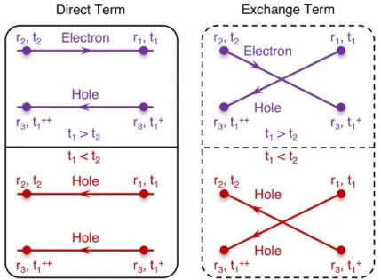
where the first and second term in the bracket on the right-hand side is the direct term and exchange term, respectively. Finally, we can easily use Figure 2.2 to interpret this interacting part, which indicates that each particle is allowed to propagate independently according to the one-particle Green’s function.
Figure 2.2 | Direct term and exchange term in the interacting part of the EOM for one-particle Green’s function.
Let’s first consider the direct term in the EOM for the one-particle Green’s function as an approximation to the two-particle Green’s function, i.e. just consider the direct part:
𝛿(𝑡1+− 𝑡
3)𝐺(2)(1, 3; 2, 3+) = 𝛿(𝑡1+− 𝑡3)[𝐺(1)(1, 2)𝐺(1)(3, 3+)] (2.48)
By doing so, we can have the EOM for the one-particle Green’s function as the following form {[𝑖 𝜕
Note that the above expression is a simple independent-particle like equation, which is similar to the independent-particle Green’s function 𝐺0 that we had already discussed in EQUATION 2.43, but with an additional potential term, 𝑖 ∫ 𝑑3 ∙ 𝜈(1+, 3)𝐺(1)(3, 3+), which is nothing but a Hartree potential with the following formation
𝑉𝐻(1) = 𝑖 ∫ 𝑑3 ∙ 𝜈(1+, 3)𝐺(1)(3, 3+) = ∫𝑛(𝑟3, 𝑡1)
𝑟1− 𝑟3 𝑑𝑟3 (2.50) Then we can have the EOM for one-particle Green’s function as:
[𝑖 𝜕
𝜕𝑡1 − 𝐻0(𝑟1) − 𝑉𝐻(1)] 𝐺(1)(1, 2) = 𝛿(1, 2). (2.51) The next step is to take both the direct and exchange terms as an approximation to the two-particle Green’s function as shown in EQUATION 2.47. Inserting EQUATION 2.47 into EQUATION 2.39, we can have the EOM for one-particle Green’s function as:
[𝑖 𝜕
𝜕𝑡1− 𝐻0(𝑟1) − 𝑉𝐻(1)] 𝐺(1)(1, 2) + 𝑖 ∫ 𝑑3 ∙ 𝜈(1+, 3)𝐺(1)(1, 3+)𝐺(1)(3, 2) = 𝛿(1, 2)
(2.52)
where the interaction term is now a non-local operator. It can be shown that it is the Green’s function variation of the exchange interaction appearing in the Hartree-Fock approximation.100
In order to have a good understanding of the direct and exchange terms, let’s first have a look at the 𝑉𝐻(1) term in EQUATION 2.51. 𝛿(1, 2) is non-zero only if 1 ≡ 2. Thus, the particle
(electron/hole) is not going anywhere. This is actually a static state. The electron density at position 𝑟3 at time 𝑡1, 𝑛(𝑟3, 𝑡1) will affect the particle propagation from 2 → 1. Therefore, we can arrive at the expression for 𝑉𝐻(1) as in EQUATION 2.50.
electron density at position 𝑟3 at time 𝑡1+, 𝑛(𝑟
3, 𝑡1+) will affect the propagation from 3+ to 1. Thus,
we have the expression of 𝜈(1+, 3) in EQUATION 2.52.
Figure 2.3 | Interpretation of the exchange term in the interacting part of the EOM for one-particle Green’s function.
2.4.6 Self-energy operator
When we consider both the direct and exchange terms in the two-particle Green’s function, we have the EOM of the one-particle Green’s function as shown in EQUATION 2.52, now let’s reform
EQUATION 2.52 to the following form
[𝑖 𝜕
𝜕𝑡1 − 𝐻0(𝑟1) − 𝑉(1)] 𝐺(1)(1, 2) − 𝑖 ∫ 𝑑3 ∙ Σ(1, 3)𝐺(1)(3, 2) = 𝛿(1, 2) (2.53) where Σ is the self-energy operator, and 𝑉(1) can be expressed as
𝑉(1) = 𝜙(1) + 𝑉𝐻(1) (2.54)
where 𝜙(1) is any external potential (such as an experimental probe) that will vanish in the end. By comparing EQUATION 2.52 and EQUATION 2.53, one notices that we have used the self-energy operator Σ to approximate the 𝜈(1+, 3)𝐺(1)(1, 3+) term. Thus, the particle is considered to move
By using Fourier transform, we can re-write EQUATION 2.53 into the following form within energy domain
[𝜔 − 𝐻0(𝑟1) − 𝑉(𝑟, 𝜔)]𝐺(1)(𝑟
1, 𝑟2; 𝜔) − ∫ Σ(𝑟1, 𝑟3; 𝜔)G(𝑟3, 𝑟2; 𝜔)𝑑𝑟3
= 𝛿(𝑟1− 𝑟2)
(2.55)
or adopting a matrix notation
(𝜔 − 𝐻0− 𝑉)𝐺 − Σ𝐺 = 1 (2.56)
Right multiply EQUATION 2.56 by 𝐺−1, we can have the following relationship 𝐺−1= 𝜔1 − 𝐻
0− 𝑉 − Σ (2.57)
By comparing with the non-interacting expression as in EQUATION 2.49, we can further have 𝐺−1= 𝐺
0−1− Σ (2.58)
2.4.7 Dyson’s equation and quasi-particle equation
From EQUATION 2.58, we can have the following expressions via left-multiply by 𝐺0 and
right-multiply by 𝐺:
𝐺0𝐺−1𝐺 = 𝐺
0𝐺0−1𝐺 − 𝐺0ΣG (2.59)
𝐺0 = 𝐺 − 𝐺0ΣG (2.60)
𝐺 = 𝐺0+ 𝐺0ΣG (2.61)
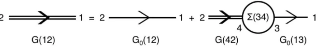
Here, EQUATION 2.61 is called the first-order Dyson’s equation. We can also have Dyson’s equation in a higher-order expansion from the second-order to the fourth-order:
𝐺(1)(𝑟
1, 𝑟2; 𝜔) = 𝐺0(1)(𝑟1, 𝑟2; 𝜔)
+ ∫ 𝐺0(1)(𝑟1, 𝑟3; 𝜔)𝛴(𝑟3, 𝑟4; 𝜔)𝐺(1)(𝑟4, 𝑟2; 𝜔)𝑑(34)
(2.65)
We can also write it within the time domain as 𝐺(1)(1,2) = 𝐺
0(1)(1,2) + ∫ 𝐺0(1)(1,3)𝛴(3,4)𝐺(1)(4,2)𝑑(34) (2.66)
Here, 𝐺0(1) is the Green’s function of a mean-field system (that we have discussed in SECTION 2.4.6) defined by the single-particle Hamiltonian ℎ̂0 with the following expression
ℎ̂0 = 𝐻0+ 𝑉𝐻 (2.67)
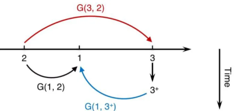
where 𝐻0 and 𝑉𝐻 are given in EQUATION 2.40 and EQUATION 2.50, respectively. We can understand this first-order Dyson’s equation easily through the Feynman diagram101 as shown in Figure 2.4.
Figure 2.4 | Feynman diagram interpretation of the first-order Dyson’s equation.
By inserting the Lehmann representation of Green’s function as in EQUATION 2.38 into
EQUATION 2.65, we see that the wave functions 𝜙𝑛(𝑟) and energies 𝜀𝑛 obey the quasi-particle
equation with the following form (derivation of quasi-particle equation is detailed in APPENDIX B) ℎ̂0(𝑟1)𝜙𝑛(𝑟1) + ∫ Σ(𝑟1, 𝑟2; 𝜀𝑛)𝜙𝑛(𝑟2)𝑑𝑟2 = 𝜀𝑛𝜙𝑛(𝑟1) (2.68)
𝜙𝑛(𝑟) and energies 𝜀𝑛 must not be understood as single-particle quantities. In fact, they are nothing but Lehmann amplitudes and excitation energies as defined in EQUATION 2.34 and
EQUATION 2.35.
2.4.8 Hedin’s equations and the GW approximation to the self-energy
Based on the Dyson’s equation, we have already established a connection between the fully interacting propagator 𝐺(1) and the propagator 𝐺0(1), where the latter is the non-interacting system through the self-energy. Through this connection, we reduced the problem of solving the Green’s function 𝐺(1) to the calculation of the self-energy. However, as mentioned above, in the
Hartree-Fock approximation of the self-energy Σ, no correlation effects have been taken into account. Thus, in order to introduce correlation effects, Hedin expressed the self-energy Σ in terms of the dynamically screened Coulomb potential 𝑊 instead of the bare Coulomb potential ν. 𝑊 is given by:
𝑊(1,2) = ∫ 𝜖−1(1,3)𝜈(3,2)𝑑(3) (2.69)
where 𝜖−1 is defined as the inverse dielectric matrix, which describes the screening of the bare
Coulomb potential due to all other electrons in the system. In 1965, Hedin102-103 showed how to derive a set of coupled integral-differential equations whose self-consistent solution, in principle, gives the exact self-energy of the system. Therefore, one can use that self-energy to calculate the Green’s function 𝐺(1). The following equations are Hedin’s equations (a detailed derivation of
Hedin’s equations is given in APPENDIX C):
𝐺(1,2) = 𝐺0(1,2) + ∫ 𝐺0(1,3)𝛴(3,4)𝐺(4,2)𝑑(3,4) (2.71)
𝛤(1,2; 3) = 𝛿(1,2)𝛿(1,3) + ∫𝛿𝛴(1,2)
𝛿𝐺(4,5)𝐺(4,6)𝐺(7,5)𝛤(6,7; 3)𝑑(4,5,6,7) (2.72) 𝑃 = −𝑖 ∫ 𝐺(2,3)𝛤(3,4; 1)𝐺(4,2)𝑑(3,4) (2.73)
𝑊(1,2) = 𝜈(1,2) + ∫ 𝜈(1,3)𝑃(3,4)𝑊(4,2)𝑑(3,4) (2.74) Here ν(1,2) = ν(𝑟1, 𝑟2)δ(𝑡1− 𝑡2) is the bare Coulomb potential, 𝛤 is the vertex function, 𝑃 is the irreducible polarizability, and 𝑊 is the screened Coulomb potential. We can easily use the diagram illustrated in Figure 2.5 to understand the relationship among these parameters in Hedin’s equations.
Figure 2.5 | Illustration of Hedin’s equations (left) and the GW approximation (right).