Identifying Local Dependence with a Score Test Statistic
Based on the Bifactor 2-Parameter Logistic Model
Yang Liu
A thesis submitted to the faculty of the University of North Carolina at Chapel Hill in partial fulfillment of the requirements for the degree of Master of Arts in the Department of Psychology
Chapel Hill 2011
Approved by:
David M. Thissen
Robert C. MacCallum
Abstract
Yang Liu: Identifying Local Dependence with a Score Test Statistic Based on the Bifactor2-Parameter
Logistic Model
(Under the direction of Dr. David M. Thissen)
Local dependence (LD) refers to the violation of the local independence assumption of most item
re-sponse models. Statistics that indicate LD between a pair of items on a test or questionnaire that is being
fitted with an item response model can play a useful diagnostic role in applications of item response
the-ory. In this paper a new score test statistic,Sb, for underlying LD (ULD) is proposed based on the bifactor
2-parameter logistic model. To compare the performance of Sb with the score test statistic (St) based on a
threshold shift model for surface LD (SLD), and the LDX2
statistic, we simulated data under null, ULD,
and SLD conditions, and evaluated the null distribution and power of each of these test statistics. The
re-sults summarize the null distributions of all three diagnostic statistics, and their power for approximately
matched degrees of ULD and SLD. Future research directions are discussed, including the straightforward
generalization ofSbfor polytomous item response models, and the challenges involved in the corresponding
Acknowledgement
I would like to show my gratitude to my advisor Dr. David M. Thissen, former and current members of
his lab, and committee members–Dr. Robert C. MacCallum and Dr. Abigail T. Panter–for their advices in
developing the idea and programming. Also this thesis would not have been possible without my parents
and my fiancée “Flora” Meng Xu’s encouragement and support.
Table of Contents
Page
List of Tables . . . vi
List of Figures . . . vii
i. Introduction . . . 1
1. Local dependence . . . 1
2. Existing methods to identify LD . . . 2
3. Theory of score test . . . 5
ii. Method . . . 8
1. Simulation design . . . 8
2. Evaluation of LD statistics . . . 10
iii. Results . . . 10
1. Locally independent data . . . 10
2. Surface LD data . . . 12
3. Underlying LD data . . . 15
iv. Discussion . . . 18
Appendices . . . 20
List of Tables
Page
1 Two-way marginal tables for itemspandq . . . 4
2 Conditions under the null case . . . 9
3 Conditions under the ULD and SLD cases . . . 9
4 Empirical quantiles of the null distribution of the three statistics . . . 11
List of Figures
Page
1 Path diagrams: (a) Bifactor model; (b) Threshold-shift model . . . 2
2 Bivariate profile log-likelihood surfaces . . . 8
3 Empirical cdf plots . . . 12
4 ROC curves for weak SLD (δpq=0.16) . . . 13
5 ROC curves for medium SLD (δpq=0.34) . . . 14
6 ROC curves for strong SLD (δpq=0.66) . . . 15
7 ROC curves for weak ULD (apq=0.54) . . . 16
8 ROC curves for medium ULD (apq=0.96) . . . 17
Introduction
1
.
Local dependence
Item response theory (IRT) provides a collection of latent variable models and statistical procedures
(in-cluding parameter estimation techniques, model evaluation methods and diagnostics) used for item analysis
and test scoring (Thissen & Steinberg, 2009). One basic assumption of IRT models is local independence
(LI), which requires that responses to different items are independent conditional on the latent variable of
interest1
. Formally, LI implies the probability of observing responsesx={x1, . . . ,xj}to allJitems givenθto
be the product of each item’s trace line functionTj(·):
L(θ;x)=
J
Y
j=1
Tj(xj|θ) (1)
Equation1formalizes the strong version of LI (SLI; McDonald,1982). SLI serves as the basis for both
estimating item parameters and scoring, where the likelihood function of the overall response pattern for a
givenθis usually treated as though the contribution of each item is independent. Although SLI is important,
there is no feasible statistical procedure to test it, for there must be no interaction among item responses in all
marginal tables (from two-way toJ-way). Consequently, only violations of pairwise independence in certain
parametric forms, that will be introduced in the next section, are tested in practice.
Thissen et al. (1992) distinguished two substantive types of local dependence: underlying local
depen-dence (ULD) and surface local dependepen-dence (SLD). ULD refers to the scenario where an additional latent
variable can be employed to explain the error covariance within each locally dependent set of items. A
read-ing comprehension test is a typical example of ULD: Responses to items followread-ing the same text will be more
correlated due to context similarity. In contrast, SLD arises when the response to an item is fostered (i.e.
positive SLD) or hampered (i.e. negative SLD) by responses to previous items. One frequently cited example
of positive SLD involves redundant items: that is, (nearly) the same question asked more than once in a test.
Negative SLD, on the other hand, is in general less common and may be difficult to explain.
1
2
.
Existing methods to identify LD
2.1 Models
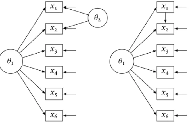
The difference between underlying and surface LD can be described using a path diagram2
. The path
diagram in Figure1illustrates the bifactor model (left), which implies ULD, and the threshold shift model
(right), which implies SLD.
θ1
x1
x2
x3
x4
x5
x6
θ2
θ1
x1
x2
x3
x4
x5
x6
Figure1: Path diagrams: (a) Bifactor model; (b) Threshold-shift model
The bifactor model is a special multidimensional factor analysis model (Gibbons & Hedeker,1992, for
the more general two-tier model, see Cai (2010)). The specification of the item bifactor model parallels the
notion of ULD in the sense that an extra latent variableθ2produces residual covariances (for a certain subset
of items) when the data are fitted with a unidimensional model. A two-parameter logistic (2PL) version of
the bifactor model for item pairpandqis:
( Tp(1|θ1, θ2)=
1
1+exp(−apθ1−apqθ2−cp)
Tq(1|θ1, θ2)=
1
1+exp(−aqθ1±apqθ2−cq)
(2)
In order to identify the model when the LD subset comprises only two items, some constraint must be
imposed on the two secondary dimension slope parameters. A convenient restriction may be equality of
the absolute value of bifactor slopes. The negativity/positivity of theapqθ2 term in the second formula is
determined by positive/negative LD to be modeled.
The2PL model is a special case of bifactor model obtained by settingapq=0in Equation2. In addition,
it can be proved (see Appendix A) that the bifactor model is equivalent to the error covariance model (see
below) in the continuous and probit case. Another parameterization of a restricted bifactor model was given
2
by Bradlow, Wainer & Wang (1999), in which bifactor slopes are fixed to be equal to their corresponding
primary slope, and the variance of the secondary factor is estimated.
The development ofa threshold shift modelmay be traced back to the work of Kelderman (1984) and
Jannarone (1986) on the Rasch model. It also appeared later in work by Hoskens & De Boeck (1997), where
it was called an “ordered-constant” interaction model, among four types of item response models employing
additional pairwise interaction parameters. Glas & Suárez Falcón (2003) derived a score test for this model’s
interaction term (see also vanaderaLinden & Glas,2010).
In the2PL case, for example, the trace line function of the second item in a locally dependent item pair
pandq(p<q) may be written as:
Tq(1|θ1;xp)=
1
1+exp(−aqθ1−cq−δpqxp) (
3)
whereδpqcan be considered a “threshold shift” for the second item when the first item response is positive,
which is in accordance with the scenario of SLD.δpqis also an ANOVA-like interaction term when the log
odds of the pairwise response pattern is considered3
. Notice that ifδpq=0, the threshold shift model reduces
to2PL model as well.
Apart from these models, there are other limited or full information parametric models for LD. For
example, both LISREL and Mplus can handle error covariances in a factor analysis model with ordered
categorical indicators based on the polychoric correlation matrix (Christoffersson,1975; Muthén,1978; see
Wirth & Edwards (2007) for a review); Braeken, Tuerlinckx, and De Boeck (2007) proposed to estimate the
dependency parameter of the bivariate logistic distribution constructed with copula functions.
2.2 Statistical procedures
Asymptotic tests: Letη=(η0,η1)be the model parameters defined in some parameter spaceΘwhich
can be factored into the direct product of subspacesΘ0×Θ1such thatη0 ∈ Θ0 andη1 ∈Θ1. Consider the
hypothesis testing problem based on a partition of the subspaceΘ1={ϑ1}∪{ϑ1}c, in which{ϑ1}cis the relative
complement of{ϑ1}inΘ1.
H0:η1 =ϑ1 (Null model)
H1:η1 ,ϑ1 (Alternative model)
Three asymptotic test statistics are commonly used for this testing problem. The likelihood ratio statistic
3
This is Hoskens & De Boeck’s interpretation; however, it is less intuitive. So I will call it the “threshold shift model” for the rest of this paper.
(Neyman & Pearson,1928) is defined as
Λ(ˆη)=
supη0∈Θ0L(η0,ϑ1;x) sup(η
0,η1)∈ΘL(η0,η1;x)
= LΘ0(η˜0,ϑ1;x) LΘ0×Θ1(ηˆ0,ηˆ1;x)
(4)
where(ηˆ0,ηˆ1) = ηˆ is the maximum likelihood estimate (MLE) inΘ, while(˜η0,ϑ1) = η˜ is the conditional
MLE obtained under the restrictionη1=ϑ1. The Wald statistic is (Wald,1943)
W(ˆη1)=(ηˆ1−ϑ1) 0H
Θ1(ηˆ1,ηˆ1)(ˆη1−ϑ1) (5)
whereHΘ1(ηˆ1,ηˆ1)is the lower-right block of the Hessian matrix of the log-likelihood. Finally, the score test
statistic (Rao,1948) is
S(η)=∇0Θ(˜η;x)H−Θ1(η˜,η˜)∇Θ(˜η;x) (6)
where∇Θ(η˜;x)is the Fisher’s score function
∇Θ(˜η;x)=∂`Θ(η;x)
∂η
η=η˜ =
∂logLΘ(η;x)
∂η
η=η˜
(7)
andH−1
Θ(η˜,η˜)is the inverse of the Hessian matrix (evaluated atη˜). It can be proved (see Buse,1982) that
like-lihood ratio, Wald, and score statistics are all asymptoticallyχ2
distributed with degrees of freedom equal to
the number of constraints imposed byH0. However, the score test statistic does not require the computation
of the MLE which is an advantage over the other two tests when applied to LD models. Because in practice
we need to test the hypotheses for each pair of items, the process of obtaining MLEs based on each LD model
can be very time consuming for long tests.
Residual measures: In this class of procedures, the IRT model with the desired number of dimensions is
fitted first, and then diagnostic statistics for residual association are calculated. One popular residual measure
uses the LDχ2
statistics for two-way marginal tables (Chen & Thissen,1997). Using the dichotomous case as
an example, for each pair of items the2×2tables as shown in Table1can be constructed for observed and
expected frequencies:
Table1: Two-way marginal tables for itemspandq
Itemq
0 1
Itemp 0 O00 O01
1 O10 O11
Itemq
0 1
Itemp 0 E00 E01
Here, Odenotes the observed frequencies andEthe expected ones. Expected cell counts are calculated according to the locally independent item response model:
Expxq=N
Z
Tp(xp|θ)Tq(xq|θ)φ(θ)dθ (8)
Basically, LDχ2
statistics reflect the discrepancy between the observed and the model-implied expected
counts. Chen and Thissen proposed the PearsonX2
and likelihood ratioG2
for this purpose:
X2 =
1 X
xp=0 1 X
xq=0
(Oxpxq−Expxq)
2 Expxq
(9)
G2 =−2
1 X
xp=0 1 X
xq=0
Oxpxqlog
Ex
pxq
Oxpxq
(10)
The theoretical null distributions for bothX2
andG2
remain unclear so far. Chen and Thissen suggested
using theχ2
-distribution with one degree of freedom as an approximation (for dichotomous items) based on
their simulation results. They claimed that the degree of freedom is one for test of independence, whereas
estimating slope parameters from the relationships among items could be regarded as imposing fractional
loss of the one degree of freedom.
There are other residual diagnostics. For example, Yen’sQ3(1984) is defined as the sample Pearson
correla-tion between paired residuals. However, it has the same problem as LDX2
andG2
, that the null distribution
of the residual correlation is not clear for categorical data4
. Another residual diagnostic, the DIMTESTT
statistic, was proposed by Stout (1987) for testing unidimensionality. As compared to Yen’sQ3, DIMTEST is
a nonparametric procedure testing whether the average residual covariance in a given item subset is
signifi-cantly larger than zero.
The research described here investigates the feasibility and usefulness of a score test for ULD, and
com-pares its performance to the score test for SLD proposed by Glas & Suárez Falcón (2003) and LDX2statistics
(Chen & Thissen,1997).
3
.
Theory of score test
3.1 Derivatives in general form
Let the response for each item be dichotomous (xij∈ {0,1}). Bock (unpublished) gave the general form of
first order derivatives taken on the marginal loglikelihood function with respect to a general item parameter
4
Yen (1984) suggested to use Fisherr-to-ztransformation, and then use standard normal distribution as an approximation. However,
subsequent studies suggested that it is actually not a good approximation (see Chen & Thissen,1997; Ip,2001).
ηs:
∂`
∂ηs =
N
X
i=1
1
Pr(xi)
∂Pr(xi)
∂ηs
=XN
i=1
1
Pr(xi)
Z
θ
∂L(xi|θ)
∂ηs
φ(θ)dθ
=
N
X
i=1
1
Pr(xi) Z
θ
XJ
j=1 xij
Tj(xij|θ)
∂Tj(xij|θ)
∂ηs
L(xi|θ)φ(θ)dθ (11)
whereL(xi|θ)=QJj=1Tj(xij|θ), andPr(xi)= R
θL(xi|θ)φ(θ)dθ. The analytical expression of the Hessian is quite
convoluted; in practice, however, the calculation of second order derivatives can be avoided by invoking the
cross-product approximation (Bock & Lieberman,1970; Kendall & Stuart,1961):
∂2`
∂ηs∂ηt ≈ −N
X
{xi}
1
Pr(xi)
∂Pr(xi)
∂ηs
∂Pr(xi)
∂ηt (12)
in which the summation is over all2J possible response patterns. This is often further approximated by
limiting the summation to observed response patterns.
3.2 Multidimensional2PL model
For2PL model, the trace line functions for binary responses can be written as (subscripti’s for subjects
are dropped):
Tj(xj|θ)=
1
1+exp[(−1)xj(a0 jθ+cj)]
(13)
The first derivatives of trace line with respect to slope and intercept parameters are listed respectively as:
∂Tj(xj|θ)
∂aj =
θTj(xj|θ)[xj−Tj(1|θ)] (14)
∂Tj(xj|θ)
∂cj =
Tj(xj|θ)[xj−Tj(1|θ)] (15)
3.3 Glas’ score statistic for threshold shift
In Glas’ threshold shift model, the trace line for the second item in an item pair is:
Tq(xq|θ,xp)=
1
1+exp[(−1)xj(a0
qθ+cq+δpqxp)] (
and the corresponding first order derivative with respect toδpqis:
∂Tq(xq|θ,xp)
∂δpq =
xpTq(xq|θ)[xq−Tq(1|θ)] (17)
3.4 The score statistic for bifactor slope
The bifactor model is a special case of multidimensional IRT model, so the derivatives of the trace line
function are described by Equation14and15.
First, we note that we cannot compute the score test from exactlyapq =0. Let(θ1, θ2)be a partition ofθ
whereθ1represents the primary factor(s)
5
andθ2the specific factor to itempandq. To evaluate
∂`
∂apq atapq=0,
notice that whenapq=0,Tj(·)and thusL(xi|θ)are constant with respect toθ2; additionally,φ(θ)=φ(θ1)φ(θ2)
due to the fact thatθ1andθ2are orthogonal. Therefore, we can write the joint integral as successive integrals
according to Fubini’s theorem6
:
∂`
∂apq
0=
N
X
i=1
1
Pr(xi) Z
θ2
θ2φ(θ2)dθ2 Z
θ1
[xip−Tp(apq|θ,xip=1)
±xiq−Tq(apq|θ,xiq=1)]L(xi|θ1)φ(θ1)dθ1
=0 (18)
It zeros out due to the fact that the first integral is the expectation of standard normal distribution, which
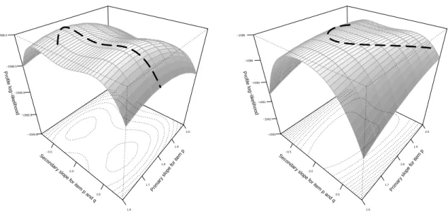
further indicates thatapq =0is either a global maximum or a saddle point. To illustrate this, the bivariate
profile log-likelihood surfaces7
of both the positive and the negative LD models as functions of(apq,ap)are
plotted as Figure2.
5
For the proofs and derivations in this section, we consider a more generic situation where there can be more than one primary factors.
6
To check the prerequisite of Fubini’s theorem, defineD(apq)=θ2[xip−Tp(apq|θ,xip)]±θ2[xiq−Tq(apq|θ,xiq)]. Then|D(apq)| ≤2|θ2|
implies the integrand is dominated.
7
The profile log-likelihood at a certain point(s,t)shown in the graphs is obtained as the restricted maximum log-likelihood after fixingapq=sandap=t.
Secondar
y slope f
or item p and q
−0.5
0.0
0.5
Primar y slope f
or item p
1.6 1.7
1.8 1.9
2.0
Profile log−lik
elihood
−1590.0 −1589.5 −1589.0 −1588.5 −1588.0
Secondar
y slope f
or item p and q
−0.5
0.0
0.5
Primar y slope f
or item p
1.6 1.7
1.8 1.9
2.0
Profile log−lik
elihood
−1593 −1592 −1591 −1590 −1589 −1588
Figure2: Bivariate profile log-likelihood surfaces for positive LD model (left; correct model for the data used
here) and negative LD model (right; wrong model for the data used here): contours (i.e. dotted lines) and
univariate profile log-likelihood curves (as a function ofapqonly; i.e. thick broken lines) are superimposed
As a result, we test the null hypothesisapq =εinstead ofapq=0, withεsome small value (0.0001in this
research). Due to the symmetry of the likelihood function with respect toapq=0, we only consider the part
thatapq > 0(which can be visualized in Figure2 as the part of log-likelihood surface on the right side of
the thick solid line) when we compute the score statistics for both positive and negative LD models. After
the two statistics associated with these two models are obtained, we check the sign of∂∂`a
pq
0.0001
to determine
which model to keep: the model with a positive value of the first derivative will be kept; if both models
produce negative value, then we consider the local independence model as the correct model.
Method
1
.
Simulation design
To investigate the performance of bifactor LD score statistics, dichotomous item response data were
gen-erated using R (R Development Core Team,2010) in three scenarios: the null case (i.e. local independence),
a ULD case, and an SLD case.
For the locally independent case, we generated test data with10,25, and50items for the sample sizes of
200,500, and1000. Item parameters were sampled from the same distributions as Chen and Thissen (1997)
are drawn from log-normal distributionloga ∼ N(0,0.5), and the thresholds (b = −c/a) are drawn from
N(0,1.5). The data generation procedure was replicated1000times for each condition; LD statistics (i.e.
bifactor score statisticSb, threshold shift score statisticSt, LDX2) were extracted only for the first item pair of
each replication.
Table2: Conditions under the null case
No. of items Sample sizes
10 200,500,1000
25 200,500,1000
50 200,500,1000
Design: No. of items×Sample sizes
ULD data were simulated using a bifactor version of the 2PL model, with only one LD pair for each
replication. Apart from sample size and number of items, we also introduced variations of the strength and
direction of LD (as shown in Table3). The strength of LD was manipulated by changing the magnitude of
secondary slopes sampled after being transformed to loadings (see Wirth & Edwards,2007):
λpq= p apq/1.702
1+(apq/1.702)2
; (19)
λpq∼ N(µλ,0.01)whereµλ=0.3,0.5,0.7, indicating low, moderate, and strong LD, respectively. In order to
obtain valid values for loadings and control the dispersion of item parameters, all these sampling
distribu-tions were truncated to the interval(µλ−0.2, µλ+0.2). As for direction, although negative LD does not have
the same substantive interpretation as positive LD, they are mathematically the same. Thus, we generate500
negative LD pairs out of the total1000replications under each simulated condition.
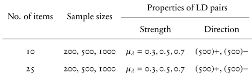
Table3: Conditions under the ULD and SLD cases
No. of items Sample sizes Properties of LD pairs
Strength Direction
10 200,500,1000 µλ=0.3,0.5,0.7 (500)+,(500)−
25 200,500,1000 µλ=0.3,0.5,0.7 (500)+,(500)−
50 200,500,1000 µλ=0.3,0.5,0.7 (500)+,(500)−
Design: No. of items×Sample sizes×Strength
Simulated conditions for SLD data are the same as ULD; however, the transformation betweenδpqand
λpq are not exact because no apparently equivalent factor analysis model is defined for the threshold shift
model. One approximation is to use the result proved (in Appendix A) with continuous indicators:
λpq= q
δpq(1−λ2
p) (20)
whereλpis the primary slope for the first item in each LD pair.
A modified version of the computational engine of the software IRTPRO was used for estimating item
parameters and computing LD statistics.
2
.
Evaluation of LD statistics
The distribution of Sb,St, andX2 under the null hypothesis can be obtained by pooling over all
repli-cations within each cell. For the locally independent case, we compare the empirical distributions to the
χ2
1 distribution
8
by means of quantiles. This shows the Type I error rates and empiricalp-values of the LD
statistics.
The receiver operating characteristic (ROC) curves of all three statistics for all conditions are presented to
provide information about the power of these tests. The horizontal axis of each of ROC curve represents the
false positive rate, or the alpha level in the setting of hypothesis testing; the vertical axis represents the true
positive rate which is the power of the statistics.
Results
1
.
Locally independent data
Several important quantiles (i.e. 0.25,0.5,0.75,0.9,0.95, and 0.999) of the empirical distributions are
tabulated for each condition of the simulation in Table4; the corresponding quantiles of theχ2
1distribution
are included in the footnote of the table.
8χ2
1is the asymptotic distribution ofSbandStaccording to the large-sample theory, as well as the approximate distribution of LDX 2
(Chen & Thissen,1997).
9
A general trend is that bothSb andSt tend to be liberal while LDX2 is conservative if the χ21 cutoffs
are used. Both increasing test length and decreasing sample size result in larger statistics, which makes the
distribution of LDX2
closer toχ2
1, but which further exacerbates the liberality of both score test statistics. The
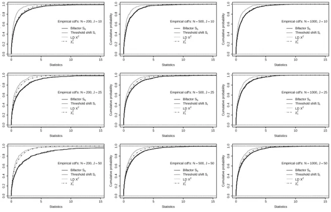
empirical quantiles ofSb andSt are nearly identical; that can be seen more clearly in empirical cumulative
density function (cdf) plots in Figure3.
0 5 10 15
0.0 0.2 0.4 0.6 0.8 1.0 Statistics Cum ulativ e probability
Empirical cdf's: N=200, J=10
Bifactor Sb Threshold shift St LD X2 χ1
2
0 5 10 15
0.0 0.2 0.4 0.6 0.8 1.0 Statistics Cum ulativ e probability
Empirical cdf's: N=500, J=10
Bifactor Sb Threshold shift St LD X2 χ1
2
0 5 10 15
0.0 0.2 0.4 0.6 0.8 1.0 Statistics Cum ulativ e probability
Empirical cdf's: N=1000, J=10
Bifactor Sb Threshold shift St LD X2 χ1
2
0 5 10 15
0.0 0.2 0.4 0.6 0.8 1.0 Statistics Cum ulativ e probability
Empirical cdf's: N=200, J=25
Bifactor Sb Threshold shift St LD X2 χ1
2
0 5 10 15
0.0 0.2 0.4 0.6 0.8 1.0 Statistics Cum ulativ e probability
Empirical cdf's: N=500, J=25
Bifactor Sb Threshold shift St LD X2 χ1
2
0 5 10 15
0.0 0.2 0.4 0.6 0.8 1.0 Statistics Cum ulativ e probability
Empirical cdf's: N=1000, J=25
Bifactor Sb Threshold shift St LD X2 χ1
2
0 5 10 15
0.0 0.2 0.4 0.6 0.8 1.0 Statistics Cum ulativ e probability
Empirical cdf's: N=200, J=50
Bifactor Sb Threshold shift St LD X2 χ1
2
0 5 10 15
0.0 0.2 0.4 0.6 0.8 1.0 Statistics Cum ulativ e probability
Empirical cdf's: N=500, J=50
Bifactor Sb Threshold shift St LD X2 χ1
2
0 5 10 15
0.0 0.2 0.4 0.6 0.8 1.0 Statistics Cum ulativ e probability
Empirical cdf's: N=1000, J=50
Bifactor Sb Threshold shift St LD X2 χ1
2
Figure3: Empirical cdf plots
From Figure3, it can be concluded thatχ2
1serves as a good approximation of the null distribution for the
score statisticsSbandStin a short test (i.e. 10items) with medium (i.e. N =500) or large (i.e. N =1000)
samples, as well as a medium length test (i.e. 25items) with large samples. Otherwise, both score statistics
are liberal. In all the conditions of this study, the empirical distributions of LDX2
are always stochastically
smaller thanχ2
1, which indicates conservativeness.
2
.
Surface LD data
0.0 0.2 0.4 0.6 0.8 1.0 0.0 0.2 0.4 0.6 0.8 1.0
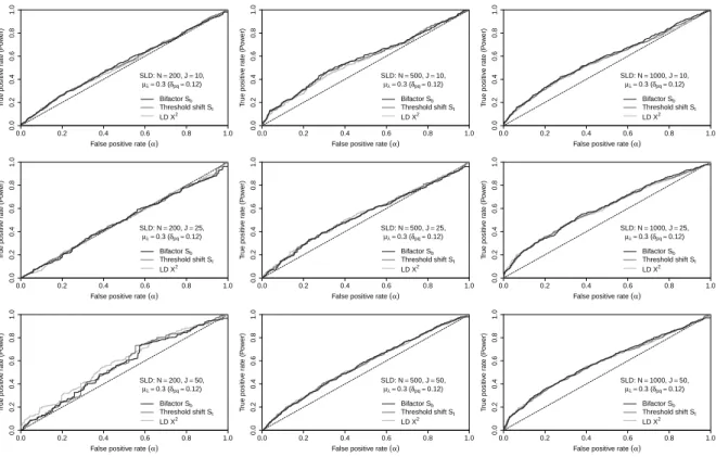
False positive rate (α)
T rue positiv e r ate (P o w er)
SLD: N=200, J=10, µλ=0.3 (δpq≈0.12)
Bifactor Sb Threshold shift St LD X2
0.0 0.2 0.4 0.6 0.8 1.0
0.0 0.2 0.4 0.6 0.8 1.0
False positive rate (α)
T rue positiv e r ate (P o w er)
SLD: N=500, J=10, µλ=0.3 (δpq≈0.12)
Bifactor Sb Threshold shift St LD X2
0.0 0.2 0.4 0.6 0.8 1.0
0.0 0.2 0.4 0.6 0.8 1.0
False positive rate (α)
T rue positiv e r ate (P o w er)
SLD: N=1000, J=10, µλ=0.3 (δpq≈0.12)
Bifactor Sb Threshold shift St LD X2
0.0 0.2 0.4 0.6 0.8 1.0
0.0 0.2 0.4 0.6 0.8 1.0
False positive rate (α)
T rue positiv e r ate (P o w er)
SLD: N=200, J=25, µλ=0.3 (δpq≈0.12)
Bifactor Sb Threshold shift St LD X2
0.0 0.2 0.4 0.6 0.8 1.0
0.0 0.2 0.4 0.6 0.8 1.0
False positive rate (α)
T rue positiv e r ate (P o w er)
SLD: N=500, J=25, µλ=0.3 (δpq≈0.12)
Bifactor Sb Threshold shift St LD X2
0.0 0.2 0.4 0.6 0.8 1.0
0.0 0.2 0.4 0.6 0.8 1.0
False positive rate (α)
T rue positiv e r ate (P o w er)
SLD: N=1000, J=25, µλ=0.3 (δpq≈0.12)
Bifactor Sb Threshold shift St LD X2
0.0 0.2 0.4 0.6 0.8 1.0
0.0 0.2 0.4 0.6 0.8 1.0
False positive rate (α)
T rue positiv e r ate (P o w er)
SLD: N=200, J=50, µλ=0.3 (δpq≈0.12)
Bifactor Sb Threshold shift St LD X2
0.0 0.2 0.4 0.6 0.8 1.0
0.0 0.2 0.4 0.6 0.8 1.0
False positive rate (α)
T rue positiv e r ate (P o w er)
SLD: N=500, J=50, µλ=0.3 (δpq≈0.12)
Bifactor Sb Threshold shift St LD X2
0.0 0.2 0.4 0.6 0.8 1.0
0.0 0.2 0.4 0.6 0.8 1.0
False positive rate (α)
T rue positiv e r ate (P o w er)
SLD: N=1000, J=50, µλ=0.3 (δpq≈0.12)
Bifactor Sb Threshold shift St LD X2
Figure4: ROC curves for weak SLD (δpq=0.16)
In Figure4, the results for weak SLD, with a threshold shift of only0.16standard units, show that there
is very little difference between the empirical curves and the diagonal line of the ROC plots (i.e. random
guess at rejecting null hypothesis) for any of the statistics, which indicates low power. Even though we gain
some power with increasing sample size, it is no more than0.2with1000observations if0.05is used as the
nominal level.
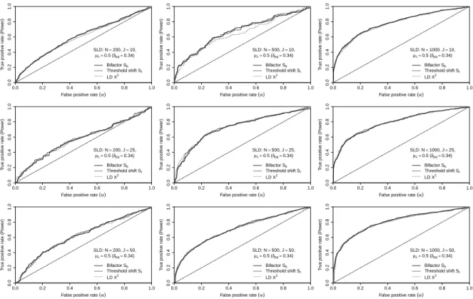
0.0 0.2 0.4 0.6 0.8 1.0 0.0 0.2 0.4 0.6 0.8 1.0
False positive rate (α)
T rue positiv e r ate (P o w er)
SLD: N=200, J=10, µλ=0.5 (δpq≈0.34)
Bifactor Sb Threshold shift St LD X2
0.0 0.2 0.4 0.6 0.8 1.0
0.0 0.2 0.4 0.6 0.8 1.0
False positive rate (α)
T rue positiv e r ate (P o w er)
SLD: N=500, J=10, µλ=0.5 (δpq≈0.34)
Bifactor Sb Threshold shift St LD X2
0.0 0.2 0.4 0.6 0.8 1.0
0.0 0.2 0.4 0.6 0.8 1.0
False positive rate (α)
T rue positiv e r ate (P o w er)
SLD: N=1000, J=10, µλ=0.5 (δpq≈0.34)
Bifactor Sb Threshold shift St LD X2
0.0 0.2 0.4 0.6 0.8 1.0
0.0 0.2 0.4 0.6 0.8 1.0
False positive rate (α)
T rue positiv e r ate (P o w er)
SLD: N=200, J=25, µλ=0.5 (δpq≈0.34)
Bifactor Sb Threshold shift St LD X2
0.0 0.2 0.4 0.6 0.8 1.0
0.0 0.2 0.4 0.6 0.8 1.0
False positive rate (α)
T rue positiv e r ate (P o w er)
SLD: N=500, J=25, µλ=0.5 (δpq≈0.34)
Bifactor Sb Threshold shift St LD X2
0.0 0.2 0.4 0.6 0.8 1.0
0.0 0.2 0.4 0.6 0.8 1.0
False positive rate (α)
T rue positiv e r ate (P o w er)
SLD: N=1000, J=25, µλ=0.5 (δpq≈0.34)
Bifactor Sb Threshold shift St LD X2
0.0 0.2 0.4 0.6 0.8 1.0
0.0 0.2 0.4 0.6 0.8 1.0
False positive rate (α)
T rue positiv e r ate (P o w er)
SLD: N=200, J=50, µλ=0.5 (δpq≈0.34)
Bifactor Sb Threshold shift St LD X2
0.0 0.2 0.4 0.6 0.8 1.0
0.0 0.2 0.4 0.6 0.8 1.0
False positive rate (α)
T rue positiv e r ate (P o w er)
SLD: N=500, J=50, µλ=0.5 (δpq≈0.34)
Bifactor Sb Threshold shift St LD X2
0.0 0.2 0.4 0.6 0.8 1.0
0.0 0.2 0.4 0.6 0.8 1.0
False positive rate (α)
T rue positiv e r ate (P o w er)
SLD: N=1000, J=50, µλ=0.5 (δpq≈0.34)
Bifactor Sb Threshold shift St LD X2
Figure5: ROC curves for medium SLD (δpq=0.34)
Figure5shows that whenδpq=0.34, there is, again, more power to detect LD in larger samples; the power
is affected very little by test length. To illustrate, choosing0.05as the nominal level and only considering
50-item tests, the power of bifactor statistics is0.11for sample size200,0.28for sample size500, and0.43for
0.0 0.2 0.4 0.6 0.8 1.0 0.0 0.2 0.4 0.6 0.8 1.0
False positive rate (α)
T rue positiv e r ate (P o w er)
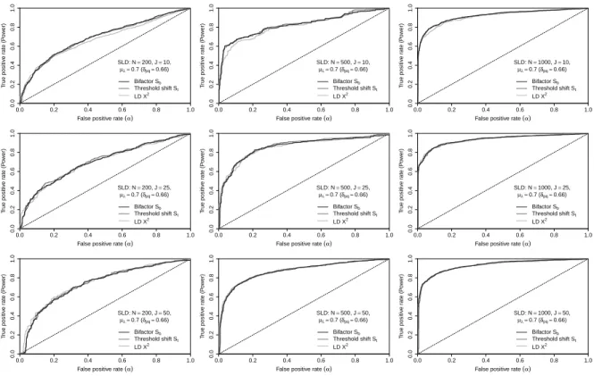
SLD: N=200, J=10, µλ=0.7 (δpq≈0.66)
Bifactor Sb Threshold shift St LD X2
0.0 0.2 0.4 0.6 0.8 1.0
0.0 0.2 0.4 0.6 0.8 1.0
False positive rate (α)
T rue positiv e r ate (P o w er)
SLD: N=500, J=10, µλ=0.7 (δpq≈0.66)
Bifactor Sb Threshold shift St LD X2
0.0 0.2 0.4 0.6 0.8 1.0
0.0 0.2 0.4 0.6 0.8 1.0
False positive rate (α)
T rue positiv e r ate (P o w er)
SLD: N=1000, J=10, µλ=0.7 (δpq≈0.66)
Bifactor Sb Threshold shift St LD X2
0.0 0.2 0.4 0.6 0.8 1.0
0.0 0.2 0.4 0.6 0.8 1.0
False positive rate (α)
T rue positiv e r ate (P o w er)
SLD: N=200, J=25, µλ=0.7 (δpq≈0.66)
Bifactor Sb Threshold shift St LD X2
0.0 0.2 0.4 0.6 0.8 1.0
0.0 0.2 0.4 0.6 0.8 1.0
False positive rate (α)
T rue positiv e r ate (P o w er)
SLD: N=500, J=25, µλ=0.7 (δpq≈0.66)
Bifactor Sb Threshold shift St LD X2
0.0 0.2 0.4 0.6 0.8 1.0
0.0 0.2 0.4 0.6 0.8 1.0
False positive rate (α)
T rue positiv e r ate (P o w er)
SLD: N=1000, J=25, µλ=0.7 (δpq≈0.66)
Bifactor Sb Threshold shift St LD X2
0.0 0.2 0.4 0.6 0.8 1.0
0.0 0.2 0.4 0.6 0.8 1.0
False positive rate (α)
T rue positiv e r ate (P o w er)
SLD: N=200, J=50, µλ=0.7 (δpq≈0.66)
Bifactor Sb Threshold shift St LD X2
0.0 0.2 0.4 0.6 0.8 1.0
0.0 0.2 0.4 0.6 0.8 1.0
False positive rate (α)
T rue positiv e r ate (P o w er)
SLD: N=500, J=50, µλ=0.7 (δpq≈0.66)
Bifactor Sb Threshold shift St LD X2
0.0 0.2 0.4 0.6 0.8 1.0
0.0 0.2 0.4 0.6 0.8 1.0
False positive rate (α)
T rue positiv e r ate (P o w er)
SLD: N=1000, J=50, µλ=0.7 (δpq≈0.66)
Bifactor Sb Threshold shift St LD X2
Figure6: ROC curves for strong SLD (δpq=0.66)
Figure6shows that as the threshold shift parameter increases to0.66, the power of all statistics becomes
higher (i.e. greater than0.6) if sample size is500or1000, but remains low/moderate (i.e. about0.25) for
small samples.
To summarize, the ROC curves of all three statistics are roughly identical, which reflects their similar
performance in all the SLD conditions. The power increases when sample size increases, but remains about
the same when test length changes.
3
.
Underlying LD data
Figures7to9show the ROC curves for the three statistics with data generated by underlying LD model.
0.0 0.2 0.4 0.6 0.8 1.0 0.0 0.2 0.4 0.6 0.8 1.0
False positive rate (α)
T rue positiv e r ate (P o w er)
ULD: N=200, J=10, µλ=0.3 (apq=0.54)
Bifactor Sb Threshold shift St LD X2
0.0 0.2 0.4 0.6 0.8 1.0
0.0 0.2 0.4 0.6 0.8 1.0
False positive rate (α)
T rue positiv e r ate (P o w er)
ULD: N=500, J=10, µλ=0.3 (apq=0.54)
Bifactor Sb Threshold shift St LD X2
0.0 0.2 0.4 0.6 0.8 1.0
0.0 0.2 0.4 0.6 0.8 1.0
False positive rate (α)
T rue positiv e r ate (P o w er)
ULD: N=1000, J=10, µλ=0.3 (apq=0.54)
Bifactor Sb Threshold shift St LD X2
0.0 0.2 0.4 0.6 0.8 1.0
0.0 0.2 0.4 0.6 0.8 1.0
False positive rate (α)
T rue positiv e r ate (P o w er)
ULD: N=200, J=25, µλ=0.3 (apq=0.54)
Bifactor Sb Threshold shift St LD X2
0.0 0.2 0.4 0.6 0.8 1.0
0.0 0.2 0.4 0.6 0.8 1.0
False positive rate (α)
T rue positiv e r ate (P o w er)
ULD: N=500, J=25, µλ=0.3 (apq=0.54)
Bifactor Sb Threshold shift St LD X2
0.0 0.2 0.4 0.6 0.8 1.0
0.0 0.2 0.4 0.6 0.8 1.0
False positive rate (α)
T rue positiv e r ate (P o w er)
ULD: N=1000, J=25, µλ=0.3 (apq=0.54)
Bifactor Sb Threshold shift St LD X2
0.0 0.2 0.4 0.6 0.8 1.0
0.0 0.2 0.4 0.6 0.8 1.0
False positive rate (α)
T rue positiv e r ate (P o w er)
ULD: N=200, J=50, µλ=0.3 (apq=0.54)
Bifactor Sb Threshold shift St LD X2
0.0 0.2 0.4 0.6 0.8 1.0
0.0 0.2 0.4 0.6 0.8 1.0
False positive rate (α)
T rue positiv e r ate (P o w er)
ULD: N=500, J=50, µλ=0.3 (apq=0.54)
Bifactor Sb Threshold shift St LD X2
0.0 0.2 0.4 0.6 0.8 1.0
0.0 0.2 0.4 0.6 0.8 1.0
False positive rate (α)
T rue positiv e r ate (P o w er)
ULD: N=1000, J=50, µλ=0.3 (apq=0.54)
Bifactor Sb Threshold shift St LD X2
Figure7: ROC curves for weak ULD (apq=0.54)
Figure 7 shows that for the weak ULD condition (apq = 0.54; error covariance is 0.09), the power is
relatively low or moderate for all cells; the power atα=0.05ranges from (approximately)0.1to0.3.
How-ever, the pattern of results is similar: Power increases as the number of observations increases, and is not
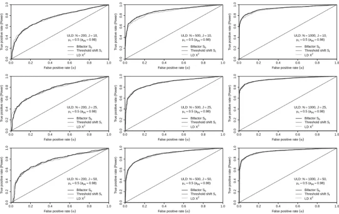
0.0 0.2 0.4 0.6 0.8 1.0 0.0 0.2 0.4 0.6 0.8 1.0
False positive rate (α)
T rue positiv e r ate (P o w er)
ULD: N=200, J=10, µλ=0.5 (apq=0.98)
Bifactor Sb Threshold shift St LD X2
0.0 0.2 0.4 0.6 0.8 1.0
0.0 0.2 0.4 0.6 0.8 1.0
False positive rate (α)
T rue positiv e r ate (P o w er)
ULD: N=500, J=10, µλ=0.5 (apq=0.98)
Bifactor Sb Threshold shift St LD X2
0.0 0.2 0.4 0.6 0.8 1.0
0.0 0.2 0.4 0.6 0.8 1.0
False positive rate (α)
T rue positiv e r ate (P o w er)
ULD: N=1000, J=10, µλ=0.5 (apq=0.98)
Bifactor Sb Threshold shift St LD X2
0.0 0.2 0.4 0.6 0.8 1.0
0.0 0.2 0.4 0.6 0.8 1.0
False positive rate (α)
T rue positiv e r ate (P o w er)
ULD: N=200, J=25, µλ=0.5 (apq=0.98)
Bifactor Sb Threshold shift St LD X2
0.0 0.2 0.4 0.6 0.8 1.0
0.0 0.2 0.4 0.6 0.8 1.0
False positive rate (α)
T rue positiv e r ate (P o w er)
ULD: N=500, J=25, µλ=0.5 (apq=0.98)
Bifactor Sb Threshold shift St LD X2
0.0 0.2 0.4 0.6 0.8 1.0
0.0 0.2 0.4 0.6 0.8 1.0
False positive rate (α)
T rue positiv e r ate (P o w er)
ULD: N=1000, J=25, µλ=0.5 (apq=0.98)
Bifactor Sb Threshold shift St LD X2
0.0 0.2 0.4 0.6 0.8 1.0
0.0 0.2 0.4 0.6 0.8 1.0
False positive rate (α)
T rue positiv e r ate (P o w er)
ULD: N=200, J=50, µλ=0.5 (apq=0.98)
Bifactor Sb Threshold shift St LD X2
0.0 0.2 0.4 0.6 0.8 1.0
0.0 0.2 0.4 0.6 0.8 1.0
False positive rate (α)
T rue positiv e r ate (P o w er)
ULD: N=500, J=50, µλ=0.5 (apq=0.98)
Bifactor Sb Threshold shift St LD X2
0.0 0.2 0.4 0.6 0.8 1.0
0.0 0.2 0.4 0.6 0.8 1.0
False positive rate (α)
T rue positiv e r ate (P o w er)
ULD: N=1000, J=50, µλ=0.5 (apq=0.98)
Bifactor Sb Threshold shift St LD X2
Figure8: ROC curves for medium ULD (apq=0.96)
Figure 8 shows that the power at nominal level 0.05 falls between0.4 to 0.8 when apq = 0.96 (error
covariance is0.25) for all the statistics, which is high compared to the medium SLD conditions. Again, all
three statistics yield similar results.
0.0 0.2 0.4 0.6 0.8 1.0 0.0 0.2 0.4 0.6 0.8 1.0
False positive rate (α)
T rue positiv e r ate (P o w er)
ULD: N=200, J=10, µλ=0.7 (apq=1.67)
Bifactor Sb Threshold shift St LD X2
0.0 0.2 0.4 0.6 0.8 1.0
0.0 0.2 0.4 0.6 0.8 1.0
False positive rate (α)
T rue positiv e r ate (P o w er)
ULD: N=500, J=10, µλ=0.7 (apq=1.67)
Bifactor Sb Threshold shift St LD X2
0.0 0.2 0.4 0.6 0.8 1.0
0.0 0.2 0.4 0.6 0.8 1.0
False positive rate (α)
T rue positiv e r ate (P o w er)
ULD: N=1000, J=10, µλ=0.7 (apq=1.67)
Bifactor Sb Threshold shift St LD X2
0.0 0.2 0.4 0.6 0.8 1.0
0.0 0.2 0.4 0.6 0.8 1.0
False positive rate (α)
T rue positiv e r ate (P o w er)
ULD: N=200, J=25, µλ=0.7 (apq=1.67)
Bifactor Sb Threshold shift St LD X2
0.0 0.2 0.4 0.6 0.8 1.0
0.0 0.2 0.4 0.6 0.8 1.0
False positive rate (α)
T rue positiv e r ate (P o w er)
ULD: N=500, J=25, µλ=0.7 (apq=1.67)
Bifactor Sb Threshold shift St LD X2
0.0 0.2 0.4 0.6 0.8 1.0
0.0 0.2 0.4 0.6 0.8 1.0
False positive rate (α)
T rue positiv e r ate (P o w er)
ULD: N=1000, J=25, µλ=0.7 (apq=1.67)
Bifactor Sb Threshold shift St LD X2
0.0 0.2 0.4 0.6 0.8 1.0
0.0 0.2 0.4 0.6 0.8 1.0
False positive rate (α)
T rue positiv e r ate (P o w er)
ULD: N=200, J=50, µλ=0.7 (apq=1.67)
Bifactor Sb Threshold shift St LD X2
0.0 0.2 0.4 0.6 0.8 1.0
0.0 0.2 0.4 0.6 0.8 1.0
False positive rate (α)
T rue positiv e r ate (P o w er)
ULD: N=500, J=50, µλ=0.7 (apq=1.67)
Bifactor Sb Threshold shift St LD X2
0.0 0.2 0.4 0.6 0.8 1.0
0.0 0.2 0.4 0.6 0.8 1.0
False positive rate (α)
T rue positiv e r ate (P o w er)
ULD: N=1000, J=50, µλ=0.7 (apq=1.67)
Bifactor Sb Threshold shift St LD X2
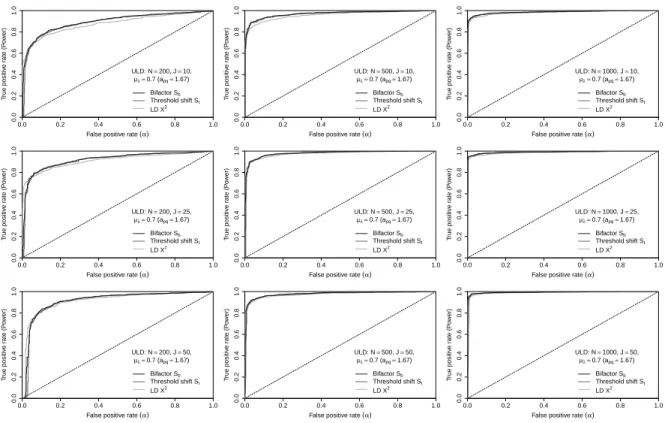
Figure9: ROC curves for strong ULD (apq=1.67)
Figure9shows that whenapqincreases to1.67(error covariance is0.49), the power for all statistics is high
for all cells; especially with large samples, all three procedures have nearly perfect power to detect underlying
LD, which is shown by their extremely steep ROC curves.
In all, the results for ULD data are similar to those obtained for SLD data; the only difference is that all
statistics seem to be more powerful here than in the corresponding SLD conditions. That may be attributed
to the approximate formula (i.e. Equation20) used to transform loadings to threshold shift parameters,
which may lead to the unmatched LD levels between the SLD and ULD data generating models.
Discussion
For locally independent data, the empirical distribution of both score test statistics closely resembles
χ2
1, especially when sample size is large and the number of items is small (which means fewer parameters are
estimated). However, we should be cautious when usingχ2
1as the null distribution in smaller samples and/or
with longer tests, because the results suggest that both score test statistics tend to be liberal. In contrast, LD
X2
is conservative if treated asχ2
however, it might be a good alternative for small samples and/or long tests.
With respect to power, all three statistics exhibit similar patterns in terms of receiver operating
character-istics, whether SLD or ULD is the data generating model. Together with the similarity of their empirical null
distributions, we conclude that both score test statistics are very close numerically. This calls the theoretical
difference between surface and underlying local dependence into question; however, further investigation is
required before reaching any conclusion about that.
In summary, all three statistics considered in this study provide useful diagnostic information about local
dependence. LDX2
is the easiest to compute and works well; its power is comparable to the score statistics,
although it is conservative whenχ2
1is used as its approximate null distribution. Both score statistics behave
similarly; however, the computation of the bifactor statisticSb requires numerically integrating over one
more dimension which makes it computationally more expensive than the threshold shift statisticSt.
In future research, it would be interesting to generalize both score test statistics to polytomous IRT
mod-els, e.g. the graded response model (Samejima,1969). The generalization of bifactor statistic is
straightfor-ward; that involves adding another dimension to the original model. In contrast, because graded response
model has more than one threshold, there are complications in generalizing the threshold shift statistic.
Sup-pose the item pair hasKresponse categories; one possibility is to incorporate different shift parameters for
each ofK−1 non-zero responses of the first item on each ofK−1 thresholds of the second item, which
leads the number of additional parameters to increase from one to(K−1)2. It might be unwieldy to explain
each of these shift parameters; nevertheless, it is acceptable to compute a multivariate score test statistic (i.e.
with limiting distributionχ2
(K−1)2) without actually obtaining parameter estimates. Other possible extensions
involve imposing constraints on the(K−1)2 shift parameters; for example, shift parameters on the same
threshold of the second item may be constrained to be equal, which results in aK−1dimensional score test
statistic. Further simulation studies are needed to evaluate these possible alternatives.
Based on all the results of the current study, we conclude that (1) LDX2is the easiest to compute, performs
well, and has been implemented in commercial software; (2) Score test statisticsSt based on the threshold
shift model is also easy to compute, and works better than LDX2
in larger samples and shorter tests; (3) Score
test statisticsSbbased on the bifactor model is the hardest to compute, and provides no advantage overStfor
dichotomous data.
Appendix 1:
Model equivalence
The equivalence of the bifactor model and the error covariance model can be established by comparing
their covariance structures. Here we only prove the simplest case in which there is only one primary
dimen-sion and one secondary dimendimen-sion (the proof can be easily generalized to multiple primary dimendimen-sions).
Consider the bifactor model:
( x∗
1=λ11θ1+λ12θ2+ε1 x∗
2=λ21θ1±λ12θ2+ε2
(21)
which has covariance structure:
Var(x∗1)=λ2 11+λ
2
12+Var(ε1) Var(x∗2)=λ2
21+λ 2
12+Var(ε2) Cov(x∗
1,x ∗
2)=λ11λ21±λ 2 12
(22)
Similarly, the error covariance model:
( x∗ 1=λ
0 11θ1+ε
0 1 x∗
2=λ 0 21θ1+ε
0 2
(23)
has covariance structure:
Var(x∗1)=λ02
11+Var(ε 0 1) Var(x∗2)=λ02
21+Var(ε 0 2) Cov(x∗
1,x ∗ 2)=λ0
11λ 0
21+Cov(ε 0 1, ε
0 2)
(24)
By equating the covariance structures (that is, Equation sets24and22), we have:
λ0
11 =λ11
λ0
21 =λ21 Var(ε01)=λ2
12+Var(ε1) Var(ε02)=λ2
12+Var(ε2) Cov(ε01, ε
0 2)=±λ2
12
(25)
The same procedure can be applied to prove the equivalence between the error covariance model and the
other than the item pair of interest. The threshold shift model is: x∗ 1=λ
00 11θ1+ε
00 1 x∗
2=λ 00
21θ1+β21x ∗ 1+ε
00 2 x∗
1=λ 00 31θ1+ε
00 3
(26)
with covariance structure:
Var(x∗1)=λ002 11 +Var(ε
00 1) Var(x∗2)=λ002
21 +β 2 21λ
002
11 +2β21λ 00 11λ
00 21+β
2 21Var(ε
00
1)+Var(ε 00 2) Cov(x∗
1,x ∗ 2)=λ00
11λ 00 21+β21λ
002
11 +β21Var(ε 00 1) Cov(x∗
2,x ∗
3)=λ0021λ 00 31+β21λ
00 11λ31
(27)
Augmenting Equation set24with
Cov(x∗ 2,x
∗
3)=λ021λ 0
31 (28)
and then comparing them with Equation set27yields:
λ0
11 =λ 00 11
λ0
21 =λ 00 21+β21λ
00 11
λ0
31 =λ 00 31 Var(ε01)=Var(ε00
1) Var(ε02)=β21Var(ε00
1)+Var(ε 00 2) Cov(ε0
1, ε 0
2)=β21Var(ε00 1)
(29)
The last equation above together with Equation set 25justifies the transformation between threshold
shift parameter (i.e.β21) and the error covariance, then the secondary loading.
References
Bock, R. D. Notes on parameter estimation for polytomous item responses models. Unpublished manuscript.
Bock, R. D. & Lieberman, M. (1970). Fitting a response model for N dichotomously scored items.
Psychome-trika,35,179–197.
Bradlow, E., Wainer, H. & Wang, X. (1999). A Bayesian random effects model for testlets. Psychometrika,64,
153–168.
Braeken, J., Tuerlinckx, F. & De Boeck, P. (2007). Copula functions for residual dependency. Psychometrika,
72,393–411.
Buse, A. (1982). The likelihood ratio, wald, and lagrange multiplier tests: An expository note. The American
Statistician,36(3),153–157.
Cai, L. (2010). A two-tier full-information item factor analysis model with¢aapplications.Psychometrika,75,
581–612.
Chen, W.-H. & Thissen, D. (1997). Local dependence indexes for item pairs using item response theory.
Journal of Educational and Behavioral Statistics,22(3),265–289.
Christoffersson, A. (1975). Factor analysis of dichotomized variables. Psychometrika,40,5–32.
Gibbons, R. & Hedeker, D. (1992). Full-information item bi-factor analysis.Psychometrika,57,423–436.
Glas, C. A. & Suárez Falcón, J. C. (2003). A comparison of item-fit statistics for the three-parameter logistic
model.Applied Psychological Measurement,27(2),87–106.
Hoskens, M. & De Boeck, P. (1997). A parametric model for local dependence among test items.Psychological
Methods,2(3),261–277.
Ip, E. (2001). Testing for local dependency in dichotomous and polytomous item response models.
Psychome-trika,66(1),109–132.
Jannarone, R. (1986). Conjunctive item response theory kernels.Psychometrika,51,357–373.
Kelderman, H. (1984). Loglinear Rasch model tests. Psychometrika,49,223–245.
Kendall, M. & Stuart, A. (1961).The advanced theory of statistics. Vol. II. London: Griffin.
McDonald, R. P. (1982). Linear versus nonlinear models in item response theory. Applied Psychological
Muthén, B. (1978). Contributions to factor analysis of dichotomous variables.Psychometrika,43,551–560.
Neyman, J. & Pearson, E. S. (1928). On the use and interpretation of certain test criteria for purposes of
statistical inference: Part i.Biometrika,20A(1/2), pp.175–240.
R Development Core Team (2010).R: A Language and Environment for Statistical Computing. Vienna, Austria:
R Foundation for Statistical Computing. ISBN3-900051-07-0.
Rao, C. R. (1948). Large sample tests of statistical hypotheses concerning several parameters with application
to problems of estimation.Proceedings of the Cambridge Philosophical Society,44,50–57.
Samejima, F. (1969). Estimation of ability using a response pattern of graded scores.Psychometrika Monograph,
No.17.
Stout, W. (1987). A nonparametric approach for assessing latent trait unidimensionality. Psychometrika,52,
589–617.
Thissen, D., Bender, R., Chen, W., Hayashi, K. & Wiesen, C. A. (1992). Item response theory and local
dependence: A preliminary report. Research memorandum, L. L. Thurstone Psychometric Lab, the
University of North Carolina at Chapel Hill, Chapel Hill.
Thissen, D. & Steinberg, L. (2009). Item response theory. In R. Millsap & A. Maydeu-Olivares (Eds.),The
Sage handbook of quantitative methods in psychology(pp.148–177). London: Sage Publications.
vanaderaLinden, W. & Glas, C. (2010). Statistical tests of conditional independence between responses
and/or response times on test items.Psychometrika,75,120–139.
Wald, A. (1943). Tests of statistical hypotheses concerning several parameters when the number of
observa-tions is large. Transactions of the American Mathematical Society,54(3),426–482.
Wirth, R. & Edwards, M. C. (2007). Item factor analysis: Current approaches and future directions.
Psycho-logical Methods,12(1),58–79.
Yen, W. M. (1984). Effects of local item dependence on the fit and equating performance of the
three-parameter logistic model.Applied Psychological Measurement,8(2),125–145.