MapReduce and Big Data: an overview

(1)

MapReduce and Big Data: an overview

Tobia Tesan

Abstract

In this document we discuss the MapReduce paradigm and its relationship with Big Data.

In Section 1 we give a general idea of what Big Data is and discuss its challenges and potential; in particular, in subsection 1.2 we give reasons why IoT should be considered closely related to Big Data.

In Section 2 we introduce the MapReduce programming paradigm and discuss its applicability, advantages and limitations; particularly, in 2.3.1 we highlight its relationship with parallel relational databases.

Finally, in Section 3, we briefly discuss the Hadoop implementation of MapRe-duce and give an example of a MapReMapRe-duce program.

List of Figures

1 Basic flow of a MapReduce computation . . . 5

2 The YARN stack of technologies (from [Whi12]) . . . 8

3 Architecture of a multi-node Hadoop cluster . . . 9

4 Snippet of input file, with fields removed . . . 13

(2)

List of Listings

1 RankDegrees class with main method . . . 10

2 CountMapper class . . . 11

3 CountReducer class . . . 11

4 RankMapper class . . . 12

(3)

1 Big Data

Ronald Fisher is famously quoted as stating, in his Presidential Address to the First Indian Statistical Congress, that “to consult the statistician after an experiment is finished is often merely to ask him to conduct a post mortem examination”, as he can at best “say what the experiment died of”.

Yet the premise of big data is that valuable information can be extracted from data which is not the result of a carefully designed experiment – and it’s the “bigness” of the data that makes this approach at once possible, necessary and challenging.

Big Data is a naturally emerging byproduct of digital interaction and not the result of a purposeful experiment – web server logs, clinical databases and in general large corpi (or corpuses) of text can be examples of big data.

As such, another key characteristic of big data is its being only partially structured. It can also be characterized [LJ12] as noisy, dynamic, heterogeneous, interrelated, untrustworthy – and, of course, big in terms of sheer size.

1.1 The challenges of Big Data: Volume, Variety and Velocity

Famously, [GP11] summarizes the challenges of big data as “volume, variety and velocity”. It’s indeed its size, or volume, that makes it valuable, potentially more than a true statistical sample of small size: as [LJ12] put it, “general statistics obtained from frequent patterns and correlation analysis usually overpower individual fluctuations and often disclose more reliable hidden patterns and knowledge”.

Yet, its volume is a challenge – more precisely, its increasing volume in the face of non-increasing compute resources at the single core level [LJ12].

It’s worth noting that the “end of Moore’s law” is happening at the same time as the shift towards cloud storage and the third, simultaneus shift towards flash storage.

This requires that algorithms and computing models used to process big data be able to exploit parallelism and are fit to be deployed in an heterogeneous environment char-acterized by multi-tenancy and where elastic scalability is a requirement – this privileges high level, declarative approaches that lend themselves well to automatic balancing and optimization.

The variety of big data – i.e. heterogeneity of formats and potential incompleteness of records – makes designing appropriate algorithms harder than in the presence of well-structured, regular data.

Finally, its velocity requires a high acquisition rate and appropriate indexing tech-niques, so that the data can be queried in real time even when it is continuosly growing. Filtering, indexing and pre-processing at the acquisition stage can help dealing with incompleteness and velocity, but engineers must find ways to do so while guaranteeing lack of information loss; the danger is real as, after all, the notion of aggregate data is fundamentally at odds with the one, given above, of big data.

1.2 Big Data and the Internet of Things

The nature of big data and IoT makes them ideal partners in a symbiotic relationship – one that is already flourishing.

(4)

IoT applications generate precisely the kind of digital data we have described in the preceding section, but on an unprecedented scale, as devices are ubiquitous and applica-tions are potentially endless: data is no longer just a byproduct of “online” interaction and is instead continuously generated as things happen in the physical world: we could go as far as saying that IoT generates the quintessential form of big data.

To give an idea of the relevance of the phenomenon, 12 million RFID tags (used to capture data and track movement of objects in the physical world) were sold in 2011 [Dul] and Gartner estimates more than 8 billion IoT devices will be in use in 2017 [vdM17].

A consequence of this is an unprecedented potential to query data and uncover rela-tionships not only in the digital domain, but among “real life” phenomena as well.

(5)

map(1) map(2) .. . map(n) reduce(1) .. . reduce(n) input output hk, vi hk0 , v0_i h_k00 , v00 i

Figure 1: Basic flow of a MapReduce computation

2 MapReduce

MapReduce is a programming model that, for reasons that will soon be apparent, is extremely popular to process big data: its most popular implementations are by far Apache Hadoop, Disco and Spark, along – in terms of services powered and, likely, sheer number of nodes deployed – with the one internally used by Google.

MapReduce did in fact come to prominence in the late 2000s in the wake of the work of Dean and Ghemaway at Google [DG08]; the authors’ purpose was to devise a mechanism to easily process and generate large data sets on commodity hardware for the company’s internal needs; the main contribution of MapReduce was a simple interface in a functional programming style – inspired, in fact, bymapandreduceprimitives in LISP – that could be automatically parallelized.

The rationale that motivated the authors was the observation that the company’s workloads were conceptually simple computations (often no more complex than an ele-mentary SQL query) made cumbersome by the need to handle large input data, parallelize and distribute the computation.

With MapReduce, the run-time system takes care of partitioning input data, schedul-ing execution, handlschedul-ing failures and managschedul-ing communication.

The MapReduce paradigm fits naturally well with distributed file systems, and is in fact often cited in conjunction with the work on the Google File System by the same authors [GGL03].

2.1 How MapReduce works

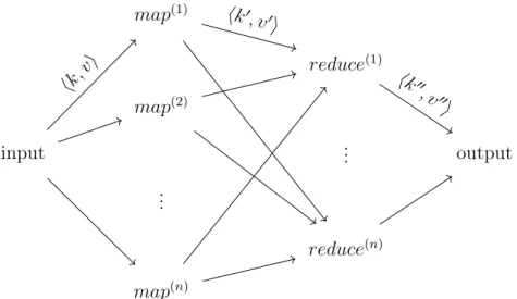
A MapReduce program is defined in terms of two functions map : hk, vi → hk0, v0i and reduce : hk0, v0i → hk00, v00i.

The MapReduce process is initated by a master node.

The input data, stored on a distributed filesystem, is first partitioned intomm-splits for processing by m map instances.

(6)

The master node maps each m-splittommap instances map(1...m) _{that yield} _m_sets of hk0, v0i pairs, each with arbitrary cardinality; the output is buffered to a local disk upon completion.

Each set is then mapped on n reduce instances reduce(1...n) _{, which the master node} initiates on worker nodes.

The reduce worker first readsall the intermediate data, it sorts the data and iteratively applies reduce : hk0, v0i → hk00, v00i over every sorted hk0, v0i pair.

Finally, the output from the various reduce jobs is written to a single output file. This computation flow is summed up in Figure 1.

Its worth noting that the algorithm described above does not require defining a schema for the input data, which can partitioned, for example, on a per-line basis, and is thus well-suited to the kind of semi-structured big data that we’ve discussed in the preceding section.

2.2 Benefits of MapReduce

MapReduce operates well in environments where bandwidth is a relatively scarce resource, as scheduling can be optimized for locality, i.e. the master node can try to initiate each worker instance on a node containing – or in the proximitiy of a node containing – a replica of the input data.

MapReduce offers a high level of resiliency to large-scale worker failures: upon failure of a node that causes loss of the intermediate map output or failure to carry a reduce job to completion, additional copies of the computations can be rescheduled on surviving nodes.

The loss of a master node is handled in the original paper through the “ostrich algo-rithm” – i.e. the possibility is ignored due to its improbability [DG08].

However, an implementation of MapReduce can easily include some form of backup or redundancy for the master node.

A distributed, non-faulting execution of a MapReduce program yields the same output as a local, sequential execution of the composition of themapandreduce function, which makes it easy to reason about Mapreduce programs, debug and test them locally.

2.3 Limitations of MapReduce

In the previous section we have detailed how declarative, high level approaches are to be favoured for deployment in the cloud; moreover, high level primitives are also essential for composing and building complex anaytical pipelines [LJ12].

MapReduce is still a relatively low level idiom that requires developers to write custom programs which – while devoid of the complexity of handling distribution and file access manually – are hard to maintain and reuse [TSJ+09].

In this respect high level languages like Hive or Pig Latin, used by Apache Pig, appear very promising: Pig Latin is a higher level procedural language, whereas Hive provides a SQL-like query language called HiveQL which supports many familiar forms of SQL statements, including SELECT, PROJECT, JOIN, AGGREGATE, UNION as well as sub-queries in the FROMclause.

(7)

RDBMS MapReduce

Volume Gigabytes Petabytes

Mode of operation Interactive and batch Batch

Mode of access R/W-many WORM

Transaction ACID No transaction support Table 1: Comparison of RDBMSs and MapReduce, from [Whi12]

Another potentially significant drawback is that deploying MapReduce on commodity nodes used for processingand storage has potentially serious consequences on the energy efficiency of MapReduce clusters.

Leverich and Kozyrakis [LK10] have highlighted how the filesystem component of MapReduce frameworks effectively precludes scale-down of clusters, as even idle nodes remain powered on all the time to ensure data availablility.

The authors have experimented modifications to the Hadoop scheduler and data lay-out that enabled them to achieve up to 50% energy savings in trade for performance, and suggested that an energy-efficient Hadoop cluster should contain a dynamic power controller which is able to intelligently optimize usage in order to assign and guarantee different service level agreements for different jobs.

2.3.1 MapReduce and parallel DBMSs

MapReduce finds itself competing in areas that, until the early 2000s, were the domain of traditional (i.e. SQL) parallel DBMSs.

However, MapReduce and SQL-based products are best considered complementary technologies suited for complementary classes of problems [SAD+10].

MapReduce is a fundamentally batch paradigm [Whi12], best suited to implement an extract-transform-load system for enormous quantities of unstructured or semistructured data rather than for fast querying of data.

Besides the edge that MapReduce has in handling semistructured data – which could be, for example, represented in traditional database systems with a wide table with many nullable attributes to accommodate multiple record types [SAD+10] – not having to define a schema makes MapReduced better suited for one-off complex data transformations.

PDBMSs also exhibit significantly higher TOC and setup costs that make MapReduce-based systems attractive [SAD+10] for users with limited budgets.

Stonebraker [SAD+_{10] however notes that PDBMSs are still the appropriate choice} for query-intensive, interactive applications.

(8)

Pig Hive

Application layer MapReduce Spark tez ...

Compute layer YARN

Storage layer HDFS HiBase

Figure 2: The YARN stack of technologies (from [Whi12])

3 Hadoop

Hadoop is an extremely popular implementation of MapReduce that was originally imple-mented as a component of Apache Nutch, directly inspired by the GFS and MapReduce papers soon after they were published by Google engineers; Hadoop was spun off Apache Nutch and became its own project in 2006 [Whi12].

Since its beginnings, Hadoop has incorporated a MapReduce implementation and a distributed filesystem called HDFS [Whi12];

Moreover, since its second version, Hadoop incorporates Apache YARN for cluster management; YARN provides low-level APIs for requesting and working with cluster resources.

In turn, these APIs are leveraged by higher level distributed computing frameworks – such as MapReduce, Spark... – that run as YARN applications on top of the YARN cluster [Whi12]; the MapReduce implementation running on YARN in Hadoop ≥ 2.x

mantains API compatibility with so-called Mapreduce 1 API.

Three layers – Application Layer, Cluster Compute Layer and Storage Layer – are thus determined, visible in Figure 2.

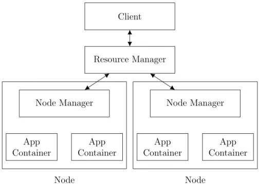
The participants in a YARN compute cluster are the Resource Manager that exposes the computing resources to clients and coordinates several Node Managers, one per cluster node; several containerized application processes are run under each Node Manager, as illustrated in Figure 3.

Application processes are not necessarily symmetrical nor independent from each other – for example, in MapReduce jobs, there is a so-called “application master” process, which has coordination responsibilities towards other processes in the same job.

3.1 An example MapReduce program: education in Italy

We will now give an example of a MapReduce program using Hadoop.

Let us note that the data we will manipulate are indeed distant from the definition of “big data” and the operations we will carry out on them are equivalent to a one-line SQL query – however, they shall make for a relatively straightfoward example.

More complex programs that processactual big data will not deviate from the paradigm that the example serves to illustrate – since, naturally, they will be subject to the same flow of control imposed by the framework – but may include more complex logic in their reduce and map functions.

(9)

Client

Resource Manager

Node Manager Node Manager

App Container App Container App Container App Container Node Node

Figure 3: Architecture of a multi-node Hadoop cluster

We have retrieved from the i.Stat datawarehouse [IST], made available by ISTAT, a 112.7MB dataset containing the census of individuals per type and level of degree obtained1_{, per gender, per age group in each geographical region.}

We will extract the total, nation-wide number of individuals for each type of degree and rank the various types of degrees by numerosity, with the aim of gaining some insight on what are the most represented specializations2_.

The dataset is in CSV format, uncommonly using a pipe (|) as separator. A snippet of the dataset is visible in Figure 4.

We will use, in fact, two jobs for a total of 2 mappers and 2 reducers: one job (Listings 2 and 3) counts the number of individuals per degree, using the degree as output key3, while the second one (Listings 4 and 5) ranks degrees by popularity.

The jobs are chained together rather crudely in the main method (Listing 1) – the first job writes its output to a temporary output directory which is then used as input for the second one.

A more sophisticated way of daisy-chaining jobs is offered by JobControl; alternately, Apache Oozie can be used, which runs as a service in the cluster [Whi12].

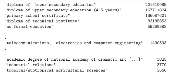
In Figure 5 we can see the resulting output, trimmed for length.

From it we can take away the reassuring notion that telecommunications engineers outnumber specialists in subtropical agriculture.

1_{Only the highest degree obtained by each individual is counted in the census}

2_{In practice, we will find that the results are inconclusive due to irregular input data – particularly, in}

some regions large numbers of individuals are simply reported to have a “Master’s Degree” or “Laurea” with no mention of the field.

3_{Note that the degree is the 13th field of a record, whereas the number of recorded individuals holding}

(10)

1 p u b l i c c l a s s RankDegrees {

2 p u b l i c s t a t i c v o i d main(String[ ] args) t h r o w s Exception {

3 i f (args.length != 2 ) {

4 System.err.println(” Usage : RankDegrees <i n p u t path> <o u t p u t ←

-path>”) ;

5 System.exit(−1) ;

6 }

7

8 Job job = new Job( ) ;

9

10 job.setJarByClass(RankDegrees.c l a s s) ;

11 job.setJobName(”Compute t o t a l c o u n t f o r e a c h d e g r e e ”) ;

12

13 FileInputFormat.addInputPath(job, new Path(args[ 0 ] ) ) ;

14 java.nio.file.Path tempnio = Files.createTempDirectory(” t o p ”) ;

15 Path temp = new Path(tempnio.toString( ) + ” / o u t p u t ”) ;

16 FileOutputFormat.setOutputPath(job, temp) ;

17

18 job.setMapperClass(CountMapper.c l a s s) ;

19 job.setReducerClass(CountReducer.c l a s s) ;

20

21 job.setOutputKeyClass(Text.c l a s s) ;

22 job.setOutputValueClass(IntWritable.c l a s s) ;

23

24 Boolean status = job.waitForCompletion(t r u e) ;

25

26 // T h i s i s a r a t h e r c r u d e way o f c h a i n i n g j o b s

27 i f (status) {

28 Job job2 = new Job( ) ;

29

30 job2.setJarByClass(RankDegrees.c l a s s) ;

31 job2.setJobName(”Rank d e g r e e s by t o t a l c o u n t ”) ;

32

33 FileInputFormat.addInputPath(job2, temp) ;

34 FileOutputFormat.setOutputPath(job2, new Path(args[ 1 ] ) ) ;

35

36 job2.setMapperClass(RankMapper.c l a s s) ;

37 job2.setReducerClass(RankReducer.c l a s s) ;

38

39 job2.setMapOutputKeyClass(IntWritable.c l a s s) ;

40 job2.setMapOutputValueClass(Text.c l a s s) ;

41

42 job2.setOutputKeyClass(Text.c l a s s) ;

43 job2.setOutputValueClass(IntWritable.c l a s s) ;

44 System.exit(job2.waitForCompletion(t r u e) ? 0 : 1 ) ;

45 } e l s e {

46 System.exit( 1 ) ;

47 }

48 }

49 }

(11)

1 p u b l i c c l a s s CountMapper

2 e x t e n d s

3 Mapper<LongWritable, Text, Text, IntWritable> {

4 @Override

5 p u b l i c v o i d map(LongWritable key, Text value, Context context) 6 t h r o w s IOException, InterruptedException {

7

8 i f (key.get( ) > 0 ) {

9 String line = value.toString( ) ;

10 String[ ] parts = line.split(Pattern.quote(”|”) ) ;

11 i f (parts.length >= 1 8 ) {

12 String degree = parts[ 1 3 ] .trim( ) ;

13 i n t number = Integer.parseInt(parts[ 1 8 ] .trim( ) ) ;

14 i f ( !degree.equals(”\” t o t a l\” ”) )

15 context.write(new Text(degree) , new IntWritable(←

-number) ) ;

16 }

17 }

18 }

19 }

Listing 2: CountMapper class

1 p u b l i c c l a s s CountReducer 2 e x t e n d s

3 Reducer<Text, IntWritable, Text, IntWritable> {

4 @Override

5 p u b l i c v o i d reduce(Text key, Iterable<IntWritable> values,

6 Context context)

7 t h r o w s IOException, InterruptedException {

8 i n t total = 0 ;

9 f o r (IntWritable value : values) {

10 total = total + value.get( ) ;

11 }

12 context.write(key, new IntWritable(total) ) ;

13 }

14 }

(12)

1 p u b l i c c l a s s RankMapper 2 e x t e n d s

3 Mapper<LongWritable, Text, IntWritable, Text> {

4 @Override

5 p u b l i c v o i d map(LongWritable key, Text value, Context context) 6 t h r o w s IOException, InterruptedException {

7 context.write(new IntWritable( 1 ) , value) ;

8 }

9 }

Listing 4: RankMapper class

1 p u b l i c c l a s s RankReducer

2 e x t e n d s

3 Reducer<IntWritable, Text, Text, IntWritable> {

4 @Override

5 p u b l i c v o i d reduce(IntWritable key, Iterable<Text> values,

6 Context context) 7 t h r o w s IOException, InterruptedException { 8 9 c l a s s Pair { 10 p u b l i c String _s; 11 p u b l i c i n t _n; 12 Pair(String s, i n t n) { 13 _s = s; 14 _n = n; 15 } 16 } 17

18 TreeMap<Integer, Pair> map = new TreeMap<Integer, Pair>() ;

19

20 f o r (Text value : values) {

21 String line = value.toString( ) ;

22 String[ ] parts = line.split(Pattern.quote(”\t ”) ) ;

23 i f (parts.length >= 2 ) {

24 Integer number = Integer.parseInt(parts[ 1 ] .trim( ) ) ;

25 String stuff = parts[ 0 ] .trim( ) ;

26 map.put(number, new Pair(stuff, number) ) ;

27 }

28 }

29

30 f o r (Pair pair : map.descendingMap( ) .values( ) ) {

31 context.write(new Text(pair._s) , new IntWritable(pair._n) ) ;

32 }

33 }

34 }

(13)

"ITTER107"|"Territory"|...|"Gen der"|...|"Certificate or degree obtained"|...|Va lue| "ITG"|"Isole"|...|"males"|...|" diploma of v ocational institute for marketing, tourism and advertising" \ |...|12235| "ITG"|"Isole"|...|"males"|...|" enterostomal therapy for professional nurses"|...|395| "ITG"|"Isole"|...|"males"|...|" laboratory technician of agricultural and food industries"|...|16| "ITG"|"Isole"|...|"males"|...|" sociopolitical field"|...|525| "ITG"|"Isole"|...|"males"|...|" other degrees of the spo rts field"|...||1321| "ITG"|"Isole"|...|"males"|...|" herbal sciences"|...|103| "ITG"|"Isole"|...|"males"|...|" environmental sciences"|...|54| "ITG"|"Isole"|...|"males"|...|" occupational therapy (qualifying course for occupational therapist healt h c\ are profession)"|...|72| "ITG"|"Isole"|...|"males"|...|" electrical engineering"|...|280| "ITG"|"Isole"|...|"males"|...|" agricultural field"|...||1245| "ITG"|"Isole"|...|"males"|...|" business and economics tele-teacher"|...|56| "ITG"|"Isole"|...|"males"|...|" diploma of v ocational institute for trade and industry"|...|49150| "ITG"|"Isole"|...|"males"|...|" science of l egal services for employment"|...|45| "ITG"|"Isole"|...|"females"|... |"degree in interpretation and translation advanced school"|...|23| "ITG"|"Isole"|...|"females"|... |"academic degree of school of fine arts (afam f irst level)"|...|441| "ITG"|"Isole"|...|"females"|... |"environmental sciences"|...|16| "ITG"|"Isole"|...|"total"|...|" total"|...|3033984| Figure 4: Snipp et of input file, with fields remo v ed

(14)

"diploma of lower secondary education" 201610085 "diploma of upper secondary education (4-5 years)" 167711824 "primary school certificate" 136087601 "diploma of technical institute" 83185853

"no formal education" 59288383

. .

"telecommunications, electronics and computer engineering" 1490593 .

.

"academic degree of national academy of dramatic art [...]" 3825

"industrial relations" 3770

"tropical/subtropical agricultural sciences" 3666

(15)

References

[DG08] Jeffrey Dean and Sanjay Ghemawat. Mapreduce: simplified data processing on large clusters. Communications of the ACM, 51(1):107–113, 2008.

[Dul] Tamara Dull. Big data and the internet of things: Two sides of the same coin? [Online].

[GGL03] Sanjay Ghemawat, Howard Gobioff, and Shun-Tak Leung. The google file system. In ACM SIGOPS operating systems review, volume 37, pages 29–43. ACM, 2003.

[GP11] Yvonne Genovese and S Prentice. Pattern-based strategy: getting value from big data. Gartner Special Report G, 214032:2011, 2011.

[IST] ISTAT. Banca Dati i.Stat. http://dati.istat.it/. Accessed: 2017-05-10. [LJ12] Alexandros Labrinidis and Hosagrahar V Jagadish. Challenges and

opportu-nities with big data. Proceedings of the VLDB Endowment, 5(12):2032–2033, 2012.

[LK10] Jacob Leverich and Christos Kozyrakis. On the energy (in) efficiency of hadoop clusters. ACM SIGOPS Operating Systems Review, 44(1):61–65, 2010.

[SAD+10] Michael Stonebraker, Daniel Abadi, David J DeWitt, Sam Madden, Erik Paul-son, Andrew Pavlo, and Alexander Rasin. MapReduce and parallel DBMSs: friends or foes? Communications of the ACM, 53(1):64–71, 2010.

[TSJ+09] Ashish Thusoo, Joydeep Sen Sarma, Namit Jain, Zheng Shao, Prasad Chakka, Suresh Anthony, Hao Liu, Pete Wyckoff, and Raghotham Murthy. Hive: a warehousing solution over a map-reduce framework. Proceedings of the VLDB Endowment, 2(2):1626–1629, 2009.

[vdM17] Rob van der Meulen. Gartner says 8.4 billion connected ”things” will be in use in 2017, up 31 percent from 2016, February 2017. [Online; posted 7-February-2017].