CHAPTER 4:
Getting adhesion force maps with an
amplitude-modulation AFM in tapping
mode
Laboratory for Energy and NanoScience
COMPENDIUM
2 LENS: Laboratory for Energy and Nano Science
LENS COMPENDIUM
Published July 2020
Authors: Matteo Chiesa1,2
Sergio Santos1,3
Chia Yun Lai1
Tuza Olukan1
Corresponding author: Matteo Chiesa -
[email protected]
,
[email protected] Affiliations:1. Department of Physics and Technology, UiT The Arctic University of Norway, Tromso, Norway
2. Laboratory for Energy and NanoScience (LENS), Khalifa University of Science and Technology, Masdar Campus, Abu Dhabi, UAE
3. Future Synthesis, Skien, Norway Design and layout: Maritsa Kissamitaki1
3 LENS: Laboratory for Energy and Nano Science
CONTENTS
Getting adhesion force maps with an amplitude-modulation AFM in tapping mode... 4
Monomodal SASS techniques
Brief introduction of Bimodal SASS techniques ... 4
Steps to collect the raw data to reconstruct force profiles ... 5
Steps to process the raw data ... 9
Examples of SASS and bimodal SASS imaging…….……….10
Bibliography ... 12
Getting adhesion force maps with an
amplitude-modulation AFM in tapping mode
4 LENS: Laboratory for Energy and Nano Science
Here we demonstrate how to get adhesion force maps with an amplitude-modulation AFM in tapping mode. Our method is tapping mode but it is carried out at ultra-small amplitudes in the presence of surface water layers. The tip is made to vibrated under the water layer in what we call Small Amplitude Small Set-point AM AFM. We show how this is done with an example based on the Cypher scanning probe microscope from Asylum Research. We also show that the elastic modulus can be simultaneously estimated while scanning by performing bimodal SASS. On top of being a quantitative method, it might enhance resolution.
Monomodal SASS techniques
Monomodal SASS can be operated in the same way as bimodal SASS by simply driving
the second mode at 0 force. In the next section we detail how to capture bimodal SASS
images taking this into consideration.
Brief introduction of Bimodal SASS techniques
A recent development in the field of Atomic Force Microscopy (AFM) relates to externally exciting multiple frequencies simultaneously while monitoring the perturbed amplitudes, phases and/or resonant frequencies1. Arguably, the most common operation mode of the family
of multifrequency AFM modes is the so-called bimodal AFM mode whereby the AFM cantilever is excited at its first and second modes. Nevertheless, while the excitation of two frequencies only is also arguably the most basic form of multifrequency AFM, the mathematical formulations involved in the derivation of simple expressions to map physical parameters2,3 is still challenging
and the proposed approximations reduce the range of valid operational parameter space4. A
more physical approach has been recently employed by two groups independently5,6 to enhance
resolution in monomodal AFM by forcing the tip of the AFM to oscillate under the nanometric water layers adsorbed on surfaces in ambient conditions. In a nutshell, the point of contact with
5 LENS: Laboratory for Energy and Nano Science
the surface is reached by immersing the tip into the water layers while maintaining the oscillations small enough that quasi-perpetual contact is achieved7. Because such mode of
operation typically involves minute oscillation amplitudes we might term it small amplitude small set-point (SASS) AFM. More recently the possibility of operating the AFM in the bimodal mode while simultaneously exploiting the advantages of SASS has been introduced theoretically8. This extension can be termed bimodal SASS (AFM). Here we set to explore the
whole small oscillation parameter space in ambient and employ bimodal SASS to enhance resolution, produce multiparametric maps and transform some of these maps into physically relevant and intuitive maps general enough to be recognized by the broader community9-14.
Steps to collect the raw data to reconstruct force profiles
1. First, insert the cantilever and fixed the cantilever holder on the Cypher head as described in the previous article.
2. Click on the BimodalDualAC tab (Figure 1). This indicates that we will operate the AFM with 2 frequencies.
Figure 1
3. Use the Igor software to put the laser spot, find the focus of the tip and the focus of the sample as described in the previous article and click the “Move to pre-engage” button.
6 LENS: Laboratory for Energy and Nano Science
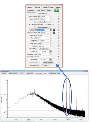
4. The cantilever should be driven at the resonance frequency. To find the natural frequency, you need to perform the Thermal test (Figure 2). After the thermal test, copy the frequency on the thermal tab and paste it in the main tab of the master panel (Figure 3) and set the drive amplitude for the 2nd mode to 0.
Figure 2: Fit the first peak in the blue oval shape.
Figure3: Paste the Thermal test result in the frequency field (red outline). Remember to set the amplitude for second mode (yellow outline) to 0.
5.
Approach the tip in the same way as described in the previous article.7 LENS: Laboratory for Energy and Nano Science
6. Perform a force-distance curve once while setting the force distance to 30 - 50 nm.
7. Perform the Thermal test again. After the thermal test, calibrate the 2nd mode first: copy the
frequency (the peak position should be around 6 times of the 1st mode) on the thermal tab
and paste it in the main tab of the master panel (Figure 3). Divide the amplitude in volts reading by 3.473 and fit the peak again to get spring constant and Q.
8. Calibrate the 1st mode: fit the
1st mode peak in the spectrum
and copy the frequency on the thermal tab and paste it in the main tab of the master panel (Figure 4). Set back to the original amplitude in volts reading and fit the peak again to get spring constant and Q.
Figure 1: Amp InvOLS during first calibration in red outline. Amp invOLS during second calibration (yellow outline) is derived by dividing value in red outline by 3.473.
9. Then, find the AC as discussed in the previous article.
8 LENS: Laboratory for Energy and Nano Science
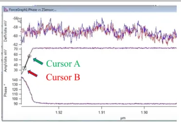
10. Find the positive slop in 1st mode amplitude versus distance curve (Figure 5) through setting the trigger point sufficiently small.
Figure 2: Find the slope by placing two cursors in the middle part of the amplitude curve. Use Ctrl + I to access the cursors and place them with the mouse.
11. Set the free amplitude to ~0.7-0.8 times of AC, and the
set-point to ~ 0.7-0.8 times of the free amplitude for the 1st
mode. For the 2nd mode, set
the free amplitude to ~0.1 times of 1st mode free
amplitude.
12. Set the phase lag in both channels to 90°.
13. Set the scan size, scan rate and gain, and start scanning. 14. Slowly decreasing the setpoint
until both 1st mode and 2nd
mode phase channel fall in repulsive regime (< 90°, Figure 6).
Figure 3: Both phase channels are below 90º.
Cursor A
9 LENS: Laboratory for Energy and Nano Science
Steps to process the raw data
Note: R studio needs to be installed and add to the path. All the source codes can be found here
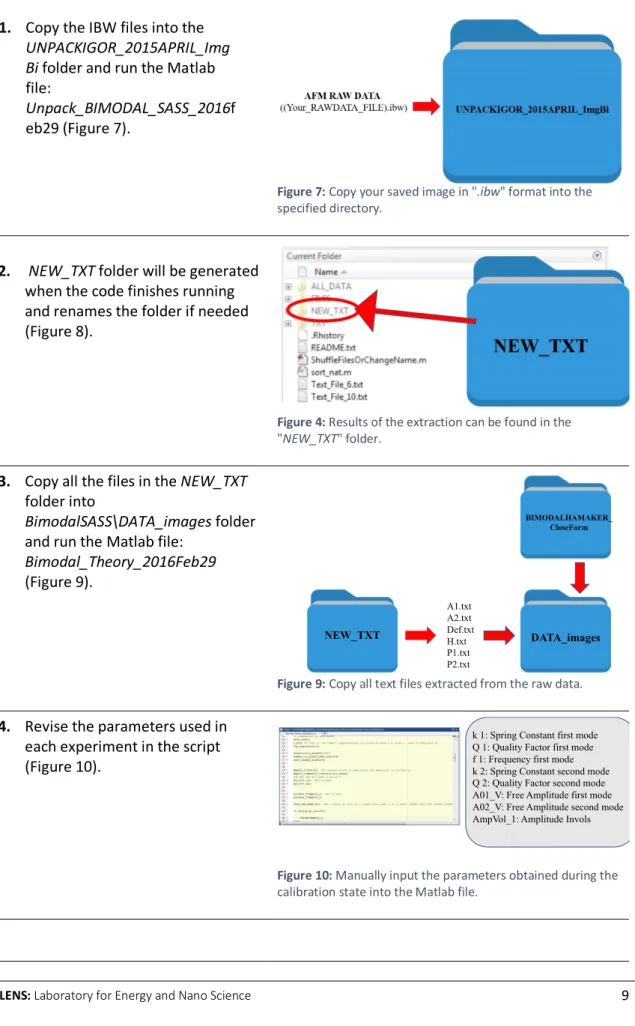
1. Copy the IBW files into the UNPACKIGOR_2015APRIL_Img Bi folder and run the Matlab file:
Unpack_BIMODAL_SASS_2016f eb29 (Figure 7).
Figure 7: Copy your saved image in ".ibw" format into the specified directory.
2. NEW_TXT folder will be generated when the code finishes running and renames the folder if needed (Figure 8).
Figure 4: Results of the extraction can be found in the "NEW_TXT" folder.
3. Copy all the files in the NEW_TXT folder into
BimodalSASS\DATA_images folder and run the Matlab file:
Bimodal_Theory_2016Feb29 (Figure 9).
Figure 9: Copy all text files extracted from the raw data.
4. Revise the parameters used in each experiment in the script (Figure 10).
Figure 10: Manually input the parameters obtained during the calibration state into the Matlab file.
A1.txt A2.txt Def.txt H.txt P1.txt P2.txt NEW_TXT DATA_images BIMODALHAMAKER_ CloseForm
k 1: Spring Constant first mode Q 1: Quality Factor first mode f 1: Frequency first mode k 2: Spring Constant second mode Q 2: Quality Factor second mode A01_V: Free Amplitude first mode A02_V: Free Amplitude second mode AmpVol_1: Amplitude Invols
10 LENS: Laboratory for Energy and Nano Science
5.
BimodalSASS\DATA_images\P rocessedData folder will be generated when the code finishes running (Figure 11).Figure 11: Generated results can be found in the "ProcessedData."
Examples of SASS and bimodal SASS imaging
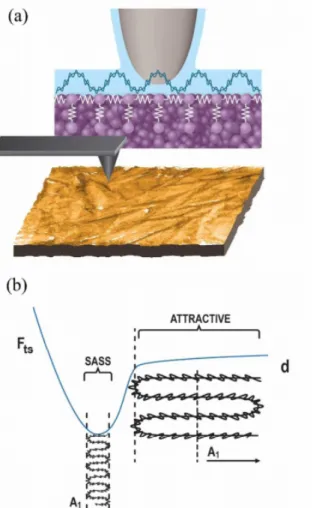
In Figure 12 we reproduce from Ref. 13 an illustration of SASS versus standard attractive
AM AFM operation.
Figure 12. (a) Illustration of an AFM tip oscillating with small amplitudes. (b) The
different operating modes when an AFM tip is oscillating in attractive and SASS regime.
11 LENS: Laboratory for Energy and Nano Science
Figure 11 illustrates why we can approximate the adhesion force to the mean deflection
of the cantilever times the spring constant Fts=kz0. Another key concept however is that
the cantilever is not in the equivalent state to quasi-static or DC AFM. This is because in
DC AFM one cannot know the adhesion force and then set a trigger force. The trigger
force is static in DC AFM and it is the feedback. In SASS the amplitude is small but not
zero so the cantilever still carries some energy in order to reach dynamic stability. Small
amplitude here means simply that the amplitude of oscillation is smaller than the range
of interest for measuring the forces, i.e. A≈0.1-0.3 nm while the force profile might be
in the order of 1 or 1 nm. Secondly, the cantilever is driven to the well by the water layer.
This was shown in simulations
8.
In SASS we can obtain both the adhesion force as shown in the well in Figure 12b and
the effective elastic modulus of the sample’s surface by applying correlating it with the
tip radius and the kinetic energy of the second mode as discussed in Ref. 13. The first
mode is sufficient to map the adhesion as one maps the topography. The second mode
is necessary to map the elastic modulus since the kinetic energy of the second mode is
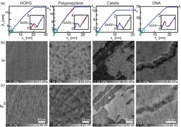
needed. An example of such maps is shown in Figure 13 as reproduced from Ref. 13 for
HOPG, polypropylene, calcite and a single DNS molecule on mica.
12 LENS: Laboratory for Energy and Nano Science
Figure 13. (a) The amplitude-distance curves obtained on HOPG, polypropylene, calcite
and DNA showing the SASS regime for AFM experiments. The calculated E* (b) and FAD
(c) maps for the four samples.
Bibliography
1
Garcia, R. & Herruzo, E. T. The emergence of multifrequency force microscopy.
Nat Nano
7, 217-226 (2012).
2
Kawai, S.
et al.
Systematic Achievement of Improved Atomic-Scale Contrast via
Bimodal Dynamic Force Microscopy.
Phys. Rev. Lett.
103, 220801 (2009).
3
Herruzo, E. T. & Garcia, R. Theoretical study of the frequency shift in bimodal
FM-AFM by fractional calculus.
Beilstein journal of nanotechnology
3, 198-206,
doi:10.3762/bjnano.3.22 (2012).
4
Aksoy, M. D. & Atalar, A. Force spectroscopy using bimodal frequency
modulation atomic force microscopy.
Physical Review B
83, 075416 (2011).
5
Wastl, D. S., Weymouth, A. J. & Giessibl, F. J. Optimizing atomic resolution of
force microscopy in ambient conditions.
Physical Review B
87, 245415 (2013).
6
Santos, S.
et al.
Stability, resolution, and ultra-low wear amplitude modulation
atomic force microscopy of DNA: Small amplitude small set-point imaging.
Appl.
Phys. Lett.
103, 063702, doi:doi:
http://dx.doi.org/10.1063/1.4817906
(2013).
13 LENS: Laboratory for Energy and Nano Science