CAS: Sequential Testing for Full Credibility

by Michael Baron and Rui Xu

ABSTRACT

This paper introduces sequential statistical methods in actuarial

science. As an example of sequential decision making that is

based on the data accrued in real time, it focuses on

sequen-tial testing for full credibility. Classical statistical tools are used

to determine the stopping time and the terminal decision that

controls the overall error rate and power of the procedure. As

a result, a set of conditions is obtained under which an insured

cohort becomes fully credible.

KEYWORDS

are deemed sufficient for decision making, without referring to other sources of information. When the real data are not sufficient,partial credibility is used according to (1.1). Compromise estimators of type (1.1) are widely used for the estimation ofpure premium, a part of the total premium, the expected amount that the insurer will have to pay to cover the policyholder’s losses during the next insured period. The resulting estimator is also called credibility pre-mium. Let us further refer to Bühlmann (1970), Bühlmann and Gisler (2005), and Herzog (2004) for foundations of credibility; and Klugman, Panjer, and Willmot (2012) and Venter (1990) for the current sta-tus of credibility theory and practice.

When does a cohort deserve full credibility? This can be determined, among other methods, by the classical limited fluctuation credibility approach. According to that approach, the cohort is fully cred-ible if its total lossS is likely to fall within a desired margin from its expected value E(S), the pure pre-mium, namely,

P S

{

−E( )S ≤cE( )S

}

≥ −1 q. (1.2)

Under theaggregate loss frequency-severity model

(Klugman, Panjer, and Willmot 2012), widely used in actuarial science, condition (1.2) for full credibil-ity can take a simple form of hypothesis testing. The model assumes X losses during the insured period, and thus the total loss amountSis the sum of a ran-dom numberX of losses with severitiesY₁, . . . ,Y_X,

.

1

∑

=

=

S Yi i

X

Assumptions.We assume a Poisson number of losses

X with the frequency parameter l = E(X). For the Poisson distribution,l also equals Var (X). The loss amounts are assumed independent of each other and independent of the number of losses, with expected value and varianceE(Y_i)= µand Var(Y_i)= s2_{. Under}

this model, E(S) = lµ, Var(S)= l(s2+ µ2_{), and the}

standardized total loss (S –E(S))/Std(S) has approxi-mately standard normal distribution, provided that

1. Introduction

Sequential statistical methods refer to data that are collected in real time. The sample size is not fixed in advance. At any moment, either a decision is taken, or it is deferred until more data become available. For example, when a statistical hypothesis is tested sequentially, after each new observation, either the null hypothesis is rejected, or it is accepted, or no decision is made at this point and sampling continues (e.g., Wald 1947; Govindarajulu 2004; Tartakovsky, Nikiforov, and Basseville 2014).

Actuaries routinely make decisions that are sequen-tial in nature (e.g., Tse 2009). During each insured period, the new claims and losses data are collected, and together with the new economic and financial situ-ation and other factors, they are taken into account for the calculation of revised premiums and risks. For all the policyholders, several decisions are made regu-larly, at least once per each insured period: whether the coverage should continue, whether the coverage should be changed, and what premium should be charged.

Conventional methods tend to ignore the facts of sequentially developing data and recurrence of actu-arial decisions. They use nonsequential statistical procedures that are based on the assumption of only one statistical inference that will not be repeated. This leads to lower than nominal confidence levels and higher than nominal probabilities of Type I and Type II errors. That is, the probability of committing an error at least once during repeated tests is substan-tially higher than the nominal level of each test. Con-trolling these errors at the specified levels is one of the benefits of the proposed sequential methodology. One important sequential problem is testing an insured cohort forfull credibility. Credibility estima-tion combines the real data R and the hypothetical prior informationH and uses acompromise estimator

(1 ) , (1.1)

= + −

C ZR Z H

methods to credibility theory. Examples of using the new tool under the popular loss models are shown in Section 3. Proposed methods are then applied to the data generated by the Actuarial Loss Simulator in Sec-tion 4. SecSec-tion 5 contains summary and conclusions, and all the lengthy proofs are found in Section 6.

2. Derivation of the sequential test

In this section, a levelα sequential test for full cred-ibility is derived. As shown in Section 1, the limited fluctuation condition for full credibility is equivalent to inequality (1.3), and thus, when deciding between the full and partial credibility, an actuary needs to conduct a test of

H c0: η ≤zq/2− δ vs H cA: η ≥zq/2, (2.1)

where

1 2

η = λ

+ γ is the tested parameter of interest,

and aregion of indifference of lengthd separates the null and alternative hypotheses. An insured cohort is consideredfully credible when there is sufficient evi-dence in the data that condition (1.3), equivalent to

H_A, is satisfied.

The sequential test of (2.1) is derived through a series of steps. First, parameterh is estimated by a statisticT_n that is based on the firstn time periods of observation. This statistic is shown to have an asymp-totically normal distribution for anyn. For most of the loss models, the distribution ofT_n contains unknown nuisance parameters which affect its variance only. In this case, the problem reduces to testing the loca-tion parameter of a normal distribuloca-tion with unknown variance, and the sequential t-test (Govindarajulu 2004, sec. 3.2; Tartakovsky, Nikiforov, and Basseville 2014, sec. 3.6.2) is applied.

2.1. Test statistic and its distribution

We assume that the claim and loss data are col-lected for a large insured cohort over a sequence of days (weeks, months). During dayk, a random number of claims X_k is observed, with random loss amounts

Y1, . . . ,YkXk. The typical actuarialfrequency-severity the number of losses is sufficient for normal

approxi-mation (Herzog 2004; Klugman, Panjer, and Willmot 2012; also see Hossak, Pollard, and Zehnwirth 1983; Longley-Cook 1962).

In view of this standardization, condition (1.2) becomes equivalent to inequality

1 2 /2, (1.3)

λ

+ γ ≥

c

zq

where γ = s/µ is thecoefficient of variation of indi-vidual losses (severity parameter), and z_q/2 is the (1 –q/2)th standard normal quantile.

Condition (1.3) is a statistical hypothesis that is being tested every insured period in order to decide on the full credibility. Conducting this test each time at a nominal level of 5% does not guarantee that the prob-ability of at least one wrong decision is within 5%. For example, there is a probability of 1 – (1 – 0.05)10

≈ 40% that a Type I error is made at least once during the course of 10 independent periods, when the prob-ability of Type I error during each period is only 5%. For this reason, we develop a sequential method

for testing for full credibility. It specifies a stop-ping time, when full credibility can be awarded to a cohort, simultaneously controlling for the probability of Type I error (assigning full credibility to a cohort that does not deserve it) and the probability of Type II error (assigning only a partial credibility whereas the full credibility should be given). As a practical result, precise criteria are derived under which an insured cohort becomes fully credible.

For some cohorts, full credibility can be granted at an early stage; for others, at a later stage. But regard-less of the time, the proposed sequential tests control the probability of Type I error at a specified level

α and the probability of Type II error at a specified levelβ. In other words, the probability that a cohort with insufficient credentials is (by a sampling error) considered fully credible is controlled at the desired level throughout the entire time of data collection and decision making.

and µm = E(Ymkj) are non-central moments of the

severity distribution form= 2, 3, 4.

The proof of this result is deferred to the Appendix. Two important conclusions follow from the form ofT_n and its asymptotic variance.

Corollary 1.The distribution of T_nis free of a scale parameter of the loss distribution.

One can see that by noticing that each fraction in (2.3) has its numerator and denominator of the same dimension. This is expected because parameter h, estimated byT_n, depends on the loss distribution only through its coefficient of variation γ. In particular, Corollary 1 implies that our decision on full credibil-ity is independent of the currency in which the losses

Y_kj are valuated.

The second conclusion is important for the prac-tical implementation of the proposed sequential scheme. In typical actuarial data, a large portion of loss amounts are entered as zeros (Sect. 8.6 of Klugman, Panjer, and Willmot 2012). In particular, this phenomenon is observed in the data obtained from the Actuarial Loss Simulator in Section 4. Zero payments are often caused by the claims exceeding policy limits or not meeting deductibles, and also by wrong coding or repeatedly submitted claims.

Allowing for a considerable probability of a zero loss clearly affects the modeling of both severities and frequencies. None of the common actuarial loss models (gamma, Pareto, log-gamma, log-normal, Burr, etc.) accounts for such a large number of zeros. Fortunately, the introduced test statisticT_n is independent of the inclusion of zero losses. Accord-ing to the next corollary, these losses can simply be deleted from the data when the test for full credibility is conducted.

Corollary 2. Let X˜_k be the actual number of claims during the k-th time period and X_k be the number of claims excluding zero losses(Y_kj= 0)for all k.Consider statistics Tn= Xn

(

1+ γ2n

)

and Tn= Xn

(

1 ˆ+ γn2

)

,

whereγ˜_nandγˆ_nare the sample coefficients of variation model assumes that the claims occur at random times,

according to a Poisson process with intensityl =E(X_k) claims per day, whereas the lossesY_kj are independent variables that follow distributionF_Y(y) with expected valueµ =E(Y_kj), variances2_{= Var(Y}

kj), and coefficient

of variationγ = s/µ, independently of claim times. Based on the observed claim frequenciesX₁, . . . ,X_n

and severitiesY₁₁, . . . , Y_1X1; . . . ;Y_n1, . . . ,Y_nX

n over

n days, parameterh is estimated by

T X

s Y

n n

n

n n n

ˆ

1 ˆ2 1 2 2 . (2.2)

= λ

+ γ = +

Here parametersl,µ, ands are estimated at timen

by the corresponding sample statistics available by that time, namely, X–_n, the average frequency or the average number of claims per time period; Y–_n and

s_n, the sample mean and sample standard deviation of severity.

This yields a sequence of statisticsT₁,T₂. . . . Besides their main purpose of testing (2.1), they can also be used for estimating the partial credibility factor

Z =ch/z_q/2 byZˆ_n=cT_n/z_q/2. This factor is applied to the compromise estimation of the pure premium whenH₀ is not rejected, and only partial credibility is assigned.

Next, we show that statisticT_n has asymptotically normal distribution under mild assumptions on the frequency and severity distributions.

Theorem 1.Suppose that the frequency variables X_k and the severity variables Y_kj are not degenerate for k= 1, . . . ,n and j= 1, . . . ,X_k;Y_kjis not a multiple of a Bernoulli random variable;E(X_k2_{)< ∞;andE(Y}

kj4)< ∞.

Then, asn→ ∞, statisticT_n is asymptotically nor-mal, and

n Tn Normal V as n

d

T

(

− η →

)

(0, ), → ∞,

where

VT

4

( )

4 , (2.3)

2

2 2 2

3

2 2

2

4 22

2 3 = µ

asLn≤(b,a). WhenLn≥a, sampling stops, andH0 is

rejected in favor of H_A. WhenLn≤b, sampling stops,

andH0 is not rejected. For a test of simple hypotheses,

whenLn does not contain unknown parameters, this

SPRT guarantees the Type I and Type II error prob-abilities ofα andβ.

Suppose for a moment that the distribution ofT_n is free of nuisance parameters. It happens, for example, when the loss model is parameterized only by a scale parameter, according to Corollary 1. In this case, the SPRT statistic for testing (2.1) is

n t f t H

f t H

n

V t

z

c t

z c

n Tn

A Tn T

q q

, , ln

2 , (2.5)

0

/2 2

( )

/2 2

(

)

(_{( )})

Λ = Λ δ =

= __ − − δ_{ − −}



  

wheret is the value ofT_n observed at timen.

Now turn to the general case of an arbitrary loss dis-tribution. As seen in Theorem 1, additional param-eters can affect the asymptotic variance but not the mean of T_n. To handle nuisance parameters, Wald (1947) proposed the method of weight functions w(q), integrating both components of the likelihood ratio with respect to the unknown parameterq,

f H w d

f H w d

n

n A n

∫

∫

( )

( )

( ) ( )

Λ = θ θ

θ θ

x

x 0 .

Then, the same stopping boundariesa andb (Fig. 1) control theintegratedType I and Type II error prob-abilities, namely,

H H w d

H HA w d

∫

∫

{

}

{

}

( ) ( )

θ θ θ = α

θ θ θ = β

P P

reject , ,

do not reject , (2.6)

0 0

0

Applying this approach to our case of a normally distributed statistic with an unknown variance, a

sequential t-test is detailed in Govindarajulu (2004, Sect. 3.2). This method essentially follows Wald’s SPRT with a special choice of a constant weight functionw(q)= 1 onq ∈(0,h). Lettingh→ ∞ yields the test statistic

based on all the observed severities and based on the no-zero severities only. Then P{T˜_n=T_n}=1 for all n.

This result follows immediately from an alterna-tive expression for statisticT_n given below.

Lemma 1. Statistic Tn= Xn

(

1 ˆ+ γn2

)

can also be

expressed as

T

n Y n Y

n k

n

j Xk

kj k

n

j Xk

kj

1 1

, (2.4)

1 1 1 1

2

∑∑

∑∑

=

= = = =

the average loss per day normalized by the root of the total of squared losses per day.

The proof is given in the Appendix. Clearly, all

Y_kj=0 can be simply dropped in (2.4) without affect-ing any sums, and Corollary 2 follows. Lemma 1 is also used in the proof of Theorem 1.

2.2. Sequential scheme

Based on the asymptotically normal distribution of test statisticT_n, a sequential test for full credibility is developed in this section. The proposed procedure follows the ideas of Wald’s sequential probability ratio test, or SPRT (Wald 1947; Govindarajulu 2004; Tartakovsky, Nikiforov, and Basseville 2014). This test is based on the log-likelihood ratio lnf(xn|HA)/

f(xn|H0), wherexn represents a vector of all the data

collected by the timen.To attain theType I error proba-bilityα and theType II error probabilityβ, the stopping boundariesa= ln((1 –β)/α) andb= ln(β/(1 –α)) are then introduced, with the following sequential decision-making strategy (Fig. 1). Sampling continues as long

Figure 1. Example of an SPRT. Stop whenLn

exceeds one of the boundaries

0

b a

n Stop, reject H0

Continue sampling

the time it will take to reach a decision. For example, choosing smaller α and/or β results in lower prob-abilities of making a Type I or a Type II error. At the same time, smallerαand β result in wider stopping boundariesa andb, according to (2.8), expanding the continue-sampling region. Thus, it will generally take longer for the statisticT_n to reach the boundaries. Then, a decision will be based on a larger sample, increasing its accuracy, in terms of lower error probabilities.

When the method of weight functions is used in the presence of nuisance parameters, the probabili-ties in the right-hand sides of (2.9) are understood in the integral form (2.6), which can also be interpreted as probabilities under the joint distribution of data and nuisance parameters.

3. Implementation for common

loss distributions

In this section, the introduced sequential testing scheme is elaborated for commonly used loss mod-els (Klugman, Panjer, and Willmot 2012)—Poisson number of losses X_k and exponential, gamma, log-normal, Pareto, or Weibull loss amounts Y_kj. Each example requires calculating the asymptotic variance

V_T according to Theorem 1, using it in the likelihood ratio statistic (2.5) or (2.7), and stating the sequential decision rule in terms ofLk orTn statistics, according

to (2.8).

3.1. Example 1: Exponential and Weibull

loss models

As a special and simple case, consider the exponen-tial loss distribution. It is special because the asymp-totic varianceV_T appears free of nuisance parameters (by Corollary 1). Indeed, whenY_kj∼ exponential (q), the moments are E(Y_kjm₎ = _m!qm_{. Substituting them}

into (2.3), we obtainV_T= 1/4 for anyq. By (2.5), the SPRT statistic in this case is

= 2

4 4 2

,

/2 2 /2 2

/2 2

2

2

n T z

c T z c n c T n z c n c n n q n q n q

(

)

Λ _ − − δ_{ −} −



 

= δ − δ + δ

f t H d f t H d

V

t z c

V n d

V

t z c

V n d

n h h Tn A h Tn h h T q T h T q T

∫

∫

∫

∫

( )

(

)

(

)

( ) ( ) ( ) ( )

Λ = θ θ

θ θ = θ − − θ         θ θ −

− − δ

   θ         θ →∞ →∞

ln lim ,

, ln lim 1 exp 2 1 exp 2 . (2.7) 0 0 0 0 /2 2 0 /2 2

As we shall see in Section 3, the limit in (2.7) can often be taken by the L’Hoˆpital’s Rule, erasing both integrals. Multiple integrals appear in the case of a multidimensional nuisance parameterq.

Based onLn, one makes a decision according to the

rule,

Reject in favor of _{if ln}1

and assign full credibility,

Accept and assign _{if ln}

1 partial credibility,

Continue observation and if ,

defer decision.

(2.8)

0

0

H H _a

H _b

b a

A

n

n

n

(

)

Λ ≥ = − β

α

Λ ≤ = _{− α}β

Λ ∈           

UntilLn exits from the interval (b,a) (which

even-tually happens with probability 1), the null hypoth-esis (2.1) is neither rejected nor accepted. During this time, the final decision is deferred, and the partial credibility factor estimated by Zˆ = cTn/zq/2 is used.

The same factor is applied ifH0 is finally accepted,

and the partial credibility is assigned.

According to Wald (1947), testing scheme (2.8) attains c z c z q q

{

}

{

}

η = − δ = α

η = = β

P P

Type I error

and Type II error (2.9)

/2

/2

Here the Type I error occurs when full credibility is given to a cohort that does not deserve it, and the Type II error means not giving full credibility where it is deserved.

nuisance shape parameterr. It can be seen that both integrals in (2.7) diverge to∞ ash → ∞, justifying application of the L’Hoˆpital’s Rule. Then, taking the limit ash→ ∞, we obtain the same formula as for the exponential distribution,

n c T

n z c

n c

n n q

4 4 2

,

/2 2

2

2

Λ = δ − δ + δ

and again,H0is rejected and full credibility is given

aftern insured periods if

T ac n

z

c c

n q

4 2 .

/2 ≥

δ + − δ

3.3. Example 3: Log-normal loss model

For Y_kj∼ log-normal (µ, s), the mth moment is

µm= exp(mµ +m2s2/2), and from (2.3),

VT 1 e e

1

4 .

2 _{3 2}

= − σ + σ

In this case, both integrals in (2.7) converge as

h→ ∞, so that the nuisance parameterq = s2 _{is being}

integrated out with the improper priorP_s2(q)= 1_(0,∞). Then the sequential probability ratio test statistic is

i

i

e e n

t z c

e e d

e e n

t z c

e e d

n

∫

∫

( )

(

)

(

)

Λ =

− + − −

− + 

  

    θ

− + − − − δ



 

− + 

 



  

 θ

∞ _{θ θ} −

θ θ

∞ _{θ θ} −

θ θ

1 4 exp

2 1 4

1 4 exp

2 1 4

0

3 1/2

2

3

0

3 1/2

2

3

In this case, there is no simple closed form for the stopping boundary forT_n; however, the inequalityb < Ln<a can be solved forTn numerically.

3.4. Example 4: Pareto loss model

For the Pareto (r, q) loss distribution, the mth moment isµm= qmG(m+ 1)G(r –m)/G(r). Substituting

into (2.3), we obtain the asymptotic variance

V r r

r r

T 1

3 4

2 6

3 4 ,

( )( )

( )( )

= − − −

− −

with stopping boundaries {b, a}. That is, sampling continues while

b n

c T

n z c

n

c a

n q

< 4 4 /2 2 < .

2

2

2 δ − δ + δ

Solving forT_n, we obtain the stopping boundaries for the statisticT_n,

bc n

z

c c

ac n

z

c c

q q

4 2 ,4 2 .

/2 /2

{

δ+ − δ δ+ − δ

}

When T_n attains the upper stopping boundary, the cohort is considered fully credible. If it attains the lower boundary, only partial credibility is assigned. Between the boundaries, the decision about the full credibility is deferred until one of the boundaries is crossed.

Similarly, the asymptotic variance V_T is constant for any Weibull distribution with a known shape parameter. For example, whenY_kj∼ Weibull (q, 1/2), themth moment isµm= qmG(1+ 2m), which leads to

V_T= 17/12 and the SPRT statistic

n c T

n z c

n c

n n q

12 17

12 17

6

17 .

/2 2

2

2

Λ = δ − δ + δ

Reject H₀ and give full credibility aftern insured periods whenLn≥a, or, equivalently,

T ac

n z

c c

n q

17

12 2 .

/2 ≥

δ + − δ

3.2. Example 2: Gamma loss model

Extending the exponential model, letY_kj∼ gamma (r,q), with themth momentµm=E(Ym)=qmG(r+m)/G(r).

Substituting these moments into (2.3) and simplifying, we obtain

V r r r

T

2

4 1 .

2

2

( )

= + +

+

As stated by Corollary 1, the asymptotic variance of

from Corollary 2, the test is independent of the appear-ance of zero losses in the data. The simulated insured records start on 01/01/2000 and continue for the next 12 years, with the insurance contract being renewed and premium being revised once a year. At these times of renewal, the credibility decisions are to be made.

Claim frequencies X_k are Poisson, and the non-zero loss amountsY_kj are generated from gamma and Pareto distributions. The limited fluctuation criterion (1.2) for full credibility is applied with the relative precision c = 0.1 and probability q = 0.05, and the corresponding hypothesis is tested with the indiffer-ence margin d = 0.02. With these parameters, test (2.1) reduces to testing

H z

c vs H

z c

q

A q

: 19.4 : 19.6.

(4.1)

0 η ≤ /2 /2

− δ _{= η ≥ =}

Thus, whether a cohort deserves full credibility is

determined by the unknown parameter

1 2

η = λ

+ γ .

Its sequential estimator T_n and the corresponding stopping boundaries are calculated according to Equation (2.2) and Table 1, and the sequential test is conducted for each data sequence resulting in a defi-nite decision on full credibility.

4.1. Gamma loss model

We start by generating a 12-year record of gamma distributed losses with shape parameterr= 20, scale parameterq = 10 (average claimµ = $200), and the frequency ofl = 600 claims per year, 20% of which are not covered. This results inh = 21.4, high enough to support full credibility, according to the limited fluctuation credibility approach.

The histogram of observed losses is on Fig. 2, where a tall column on the left reflects a large portion of uncovered claims (Y_kj= 0). As we anticipated, the null hypothesis is rejected, claiming full credibility. The test statisticT_n converges to the true value ofh = 21.4, supporting the result of Theorem 1, and quickly exceeds the upper rejection boundary. At this time (in 2001, two years after signing the first contract), the null hypothesis is rejected, and full credibility is assigned. and by the L’Hoˆpital’s Rule, the same test statistic

n c t

n z c

n c

n

q

4 4 /2 2

2

2

2

Λ = δ − δ + δ

as in the gamma case. Thus, full credibility should again be assigned as soon as

T ac n

z

c c

n

q

4 2 .

/2 ≥

δ+ − δ

Table 1 summarizes the stopping boundaries for test statisticT_n (the stopping boundary forT_n does not have a closed form in the case of a log-normal distri-bution). These are conditions that allow to assign full credibility.

4. Analysis of actuarial data

In this section, we apply the developed sequential techniques to the actuarial data generated by theCAS Public Loss Simulator. This simulator was written by Goouon under a research agreement with the Casu-alty Actuarial Society (CAS) and was made publicly available at http://www.goouon.com/loss_simulator_ project.html. It generates data sets close to the real data by simulating all the features usually observed in actu-arial records.

Below, we discuss four data sets that are generated in order to illustrate situations leading to different deci-sions on the full credibility. In these examples, we con-sider a single-payment model, where each loss event is shortly followed by valuation that results in either no payment or one payment. The probability of no payment is set top₀= 0.2, which means that roughly 20% of submitted claims are denied. As we know

Table 1. Rejection boundary (condition for full credibility) for some loss distributions

Loss distribution family Rejection boundary forcredibility when the inequality holds)Tn (Assign full Gamma (r,q)

Pareto(r,q) Tn≥₄ac_n zq_c/ 2 _2c

δ+ − δ

Weibull ,1 2

θ 

  T acn z

c c

n 17 q

12 2

/ 2 ≥

frequency of claims. Partial credibility will then be assigned with the credibility factor estimated by

Zˆ2003=cT2003/zq/2= 0.949.

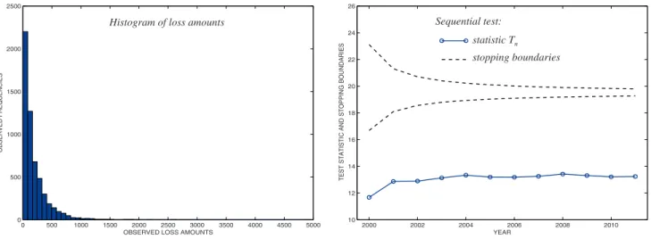
4.2. Pareto loss model, heavy tail

How will the test results of Section 4.1 change if we replace the gamma loss model with a heavy-tail distribution, say, Pareto? In this section, we again generate 12 years of claims, 01/01/2000 through 12/31/2011. As in our first example (Fig. 2), the fre-quency of claims isl = 600 per year, 20% of them are not covered, and the average covered claim amount is µ = $200. The only difference is that now the loss distribution isPareto(r = 5,q = 800) instead of gamma. Notice that under this model,E(Ykj)= q/(r – 1)

matching the gamma(20,10) expected value; how-ever, the standard deviation is much higher due

to the heavy tail,

r

r r

1 2 258.2

σ = θ

− − = compared

to gamma’sσ = θ r =44.7.

The heavy-tail loss distribution implies a higher variability of the real data, so the limited fluctuation criterion for full credibility is no longer satisfied with the same frequency of claims. Parameterh = 13.4 is much lower than the tested value in (4.1). As a result, full credibility is denied at the first opportunity (Fig. 4), and partial credibility is applied with the credibility factorZˆ₂₀₀₀=cT₂₀₀₀/z_q/2=0.60. Due to high variability Should fewer claims occur per year, their

fre-quency may be insufficient for the full credibility even if the loss distribution is the same. In the next simulation, the loss model is still gamma(r = 20,

q =10), however, the frequency is onlyl =450 claims per year, of which 20% are not covered.

Based on this data, the test statisticTn converges

to the new value ofh = 18.5, crossing the lower stop-ping boundary, as on Fig. 3. Hence, after three years of no decision, the full credibility is finally denied in 2003 due to a significance evidence of insufficient

Figure 2. Generated gamma distributed losses withk= 600 claims per year andp0= 20% of claims not

covered. Full credibility is awarded in 2001, at the first policy renewal.

0 50 100 150 200 250 300 350 400 450 0

500 1000 1500

OBSERVED LOSS AMOUNTS

OBSERV

ED

FR

EQUENCIES

2000 2002 2004 2006 2008 2010

16 17 18 19 20 21 22 23 24 25 26

YEAR

TEST

STATISTIC

A

ND

STOPPING

BOUNDARIES

Histogram of loss amounts Sequential test: statistic Tn

stopping boundaries

Figure 3. Generated gamma distributed losses withk = 450 claims per year andp0= 20%

of claims not covered. Full credibility is denied in 2003, after four years of observation.

2000 2002 2004 2006 2008 2010

16 17 18 19 20 21 22 23 24 25 26

YEAR

TE

ST S

TAT

ISTI

C A

ND S

TOP

PING

BO

UNDA

RIE

S

Sequential test: statistic Tn

l = 1300 claims per year, and again 20% of claims are denied. This is almost the minimuml required for full credibility, as the parameterh = 19.75 barely agrees with the alternative hypothesisH_A. As a result of this borderline h, it takes ten years until 2009 before the decision is made and full credibility is finally applied.

In all the considered examples, our scheme, with sequentially estimated parameters and sequentially re-tested hypotheses (2.1), eventually agreed with the standard limited fluctuation credibility approach that assumes known parameters. However, since the fre-quency and severity parameters are in practice esti-mated from the data, results can differ, and a Type I or a Type II error can occur. Probabilities of that are controlled by (2.9).

5. Conclusion

This paper introduces sequential methods in actu-arial science. It is motivated by a number of routine decisions that actuaries make at regular time inter-vals, based on sequentially collected data. Using elementary statistical tools without accounting for multiple tests, the error rate increases with the num-ber of decisions made and considerably exceeds the nominal significance level of each test. On the other hand, applying properly designed sequential tech-of loss amounts, only 60% tech-of the compromise

esti-mator of the pure premium is based on the actually observed data, and the remaining 40% have to come from other sources such as the prior distribution.

Recall that with the same frequency of claims and the same average loss, the full credibility was quickly awarded in the example on Fig. 2, where losses had gamma distribution.

With Pareto losses, the frequency of claims should be more than twice higher in order to satisfy the con-dition for full credibility. In Fig. 5, the frequency is

Figure 4. Generated Pareto distributed losses withk = 600 claims per year,p0= 20% of claims not

covered, and the average covered loss amountl = $200. Full credibility is denied after the first year of observation.

0 500 1000 1500 2000 2500 3000 3500 4000 4500 5000 0

500 1000 1500 2000 2500

OBSERVED LOSS AMOUNTS

OBSERV

ED

FR

EQUENCIES

2000 2002 2004 2006 2008 2010

10 12 14 16 18 20 22 24 26

YEAR

TE

ST

ST

AT

IS

TI

C

A

ND

S

TO

PP

IN

G

B

OU

ND

AR

IE

S

Histogram of loss amounts Sequential test: statistic Tn

stopping boundaries

Figure 5. Borderline case of Pareto loss model withk = 1300 claims per year. Full credibility is awarded in 2009, after ten years of observation.

Sequential test: statistic Tn

stopping boundaries

2000 2002 2004 2006 2008 2010

16 17 18 19 20 21 22 23 24 25 26

YEAR

TE

ST S

TAT

ISTI

C A

ND S

TOP

PING

BO

UNDA

RIE

6.2. Proof of theorem 1

This proof of asymptotic normality ofT_n is based on the multivariate central limit theorem (Lehmann 1999, theorem 5.4.4), representingT_n in terms of the sums of independent random variables.

From lemma 1, Tn=Sn Un, where Sk =

S

Xkj=1Ykj,

U_k=

S

X k j=1Y2kj,S

–

n=n–1

S

n

1Sk, andU

–

n=n–1

S

n

1Uk.

The last expression shows that statistic T_n is a smooth function of two sample means, S–_n and U–_n, that are based on i.i.d. variablesS₁,S₂, . . . and i.i.d. variablesU1,U2, . . . with

Sk Y X X

j Xk

kj k k

∑

(

)

( )= _       

 = µ = λµ,

=1

E E E E

Uk Y X X

j Xk

kj k k

∑

(

)

( )= _       

 = µ = λµ ,

=1 2

2 2

E E E E

S Y X Y X

X X k j Xk kj k j Xk kj k k k

∑

∑

( )=    +          

= σ + µ = λσ + τ µ

Var Var Var

Var( ) ,

=1 =1

2 2 2 2

E E

E

U Y X Y X

X X k j Xk kj k j Xk kj k k k

∑

∑

(

)

(

)

(

)

( ) _ _+         

µ − µ + µ

λ µ − µ + τ µ

E E

E

Var = Var Var

= Var = , =1 2 =1 2

4 22 2

4 22 2 22

and

S U S U X

S X U X

Y Y X

Y X Y X

X X X

k k k k k

k k k k

j Xk kj j Xk kj k j Xk kj k j Xk kj k

k k k

∑ ∑

∑

∑

(

)

(

)

(

)

(

)

( ) { } { } = + =     + _              

= µ − µµ + µ µ

λ µ − µµ + τ µµ

E

E E

E

E E

E

Cov( , ) Cov ,

Cov , Cov , Cov , Cov , = , =1 =1 2 =1 =1 2

3 2 2

3 2 2 2

fork= 1, 2, . . . , provided that the frequency distribu-tion has two finite moments, and the severity distri-bution has four finite moments.

niques, one can control the error rate at the specified level. Levelα and power (1 –β) sequential tests for full credibility are derived in this paper. As a result, conditions are determined under which an insured cohort becomes fully credible, according to the lim-ited fluctuation credibility approach. A stopping rule is derived when the sequential test for full credibility rejects the null hypothesis, in which case full cred-ibility can be assigned.

Although the introduced method is elaborated for credibility assessment, sequential methods in gen-eral and the proposed method of handling nuisance parameters can be applied to other areas. In any situ-ation when a decision is made as soon as the data collected to the moment shows significant evidence, one should be looking for proper sequential methods in order to control the overall error rate.

6. Appendix

6.1. Proof of lemma 1

Estimating parameter _{η = λ}

(

1_{+ γ}2

)

_with

Tn= Xn

(

1+s Yn2 n2

)

, we use the mean frequency

X–_n=n–1

S

1

n

X_kto estimate the frequency parameterln,

and the severity sample meanY–_n=

S

n

k=1

S

Xkj=1Ykj/

S

n k=1Xk

and the severity sample variance

s

Y Y

X

X Y Y

X n k n j Xk kj n k n k k n k k n j Xk kj k n j Xk kj k n k

2 =1 =1

2

=1

=1 =1 =1

2 =1 =1 2 =1 2

∑∑

∑

∑ ∑∑

∑∑

∑

(

)

= − = −       

to estimate the sample coefficient of variationγ = s/µ. Substituting this version of the sample variance intoT_n and simplifying, we obtain

T

n X

X Y Y Y

n Y Y

n k n k k n k k n j Xk kj k n j Xk kj k n j Xk kj k n j Xk kj k n j Xk kj

∑

∑ ∑∑

∑∑

∑∑

∑∑

∑∑

= + − _ _      _ _ = _ _ − − 1 , (6.1) 2 1 =1

=1 =1 =1

2 =1 =1 2 =1 =1 2 1 =1 =1 2 =1 =1 2

Applying the bivariate central limit theorem, we obtain

n Sn Un Normal

d

(

− λµ, − λµ ′ →

)

__0_{ Σ}_

0 , .

2

Next,applyingthebivariatedeltamethod(Lehmann 1999, Corollary 5.2.1) to sequences S–_n and U–_n and functionf(u,v)=uv–1/2_{, we obtain that}

n T n f S U f

N V

n

d n n

T

(

)

(

(

)

)

(

)

( )

− η = − λµ λµ

→

, ,

0,

(6.3)

2

where the asymptotic varianceV_T is derived by the bivariate delta method as follows.

For the functionf(u,v)=uv–1/2_{, we have∂f/∂u=v}–1/2

and∂f/∂v= –uv–3/2_{/2. Substitutingu}=_ES–

n= lµ and

v=EU–_n= lµ2, we obtain

V f u f u f v f v v u v u v T

(

)

(

)

(

)

(

)

(

)

(

)

= ∂ ∂ 

  Σ + ∂_∂ ∂_∂ Σ + ∂ _∂  Σ

= Σ − Σ + Σ

λ µ − µ + τ µ

λµ −

λµ λ µ − µµ + τ µµ λ µ

+λ µ λ µ − µ + τ µ

λ µ τ λ    µ

µ + µ − µµµ +

µ µ − µ µ 2 4 = 4 =

4 4 .

2 11 12 2 22 11 12 2 2 22 3

2 2 2 2

2

3 2 2 2

2 2 2

2 2

4 22 2 22

3 2 3 2 2 2 2 2 3 2 2 2

4 22

2 3

Acknowledgments

Support of this research by The Casualty Actuarial Society is greatly appreciated.

References

Bühlmann, H.Mathematical Methods in Risk Theory, New York:

Springer, 1970.

Bühlmann, H., and A. Gisler,A Course in Credibility Theory and

its Applications, Berlin: Springer-Verlag, 2005.

Govindarajulu, Z.,Sequential Statistics, Singapore: World

Sci-entific Publishing, 2004.

Herzog, T. N.,Introduction to Credibility Theory, Winsted, CT:

ACTEX Publications, 2004.

Random vectors (S_k,U_k)′ are independent, identi-cally distributed fork= 1, . . . ,n, with the finite mean vector (lµ,lµ2)′ and finite covariance matrix

VAR S U k k

(

)

(

)

(

)

Σ = _ _

= λσ + τ µ λ µ − µµ + τ µµ

λ µ − µµ + τ µµ λ µ − µ + τ µ

 

 .

(6.2)

2 2 2

3 2 2 2

3 2 2 2 4 22 2 22

The bivariate central limit theorem (e.g., theo-rem 5.2.1 of Lehmann 1999) holds for (S–_n, U–_n)′if

det(

S

) ≠ 0.

On the contrary, suppose that matrixS is singular. Then there exist coefficientsu andvsuch thatu2_+v2

≠ 0 and

uSk vUk uY vY const

j Xk kj kj

∑

(

)

+ = + = =1 2

almost surely. This implies that Var(uS_k +vU_k) = 0. On the other hand, lettingW_kj=uY_kj+vY2

kj, we have

uS vU W X

W X W W k k j Xk kj k j Xk kj k kj kj

∑

∑

( )

( )

( + )= _     + _    

= λ + τ

E E E Var Var Var Var . =1 =1 2 2

Sincel > 0 andt2_{> 0 by the conditions of this}

the-orem, the only possibility for Var(uS_k + vU_k) = 0 is that Var(W_kj) = 0 and E(W_kj) = 0, which means that

W_kj=uY_kj+vY2

kj= 0 with probability one. Solving this

equation for Y_kj, we obtain that Y_kj∈{0, –u/v} a.s.

However, this implies that the loss variableY_kjis either degenerate or it is a multiple of a Bernoulli random variable,

v uYkj

− ∼Bernoulli.

Tartakovsky, A. G., I. V. Nikiforov, and M. Basseville, Sequen-tial Analysis: Hypothesis Testing and Changepoint Detection, Boca Raton: CRC Press, 2014.

Tse, Y. K., Nonlife Actuarial Models: Theory, Methods and

Evaluation, New York: Cambridge University Press, 2009.

Venter, G. G., “Credibility,” in Foundations of Casualty

Actuarial Science, New York: Casualty Actuarial Society, 1990.

Wald, A.,Sequential Analysis, New York: Wiley, 1947.

Hossack, I. B., J. H. Pollard, and B. Zehnwirth, Introductory

Statistics with Applications in General Insurance, New York: Cambridge University Press, 1983.

Klugman, S. A., H. H. Panjer, and G. E. Willmot,Loss Models:

From Data to Decisions, 4th ed., New York: Wiley, 2012.

Lehmann, E. L.,Elements of Large-Sample Theory, New York:

Springer-Verlag, 1999.

Longley-Cook, L. H., “An Introduction to Credibility Theory,”