Chapter 4
Evaluating Analytical Data
Chapter Overview
4A Characterizing Measurements and Results
4B Characterizing Experimental Errors
4C Propagation of Uncertainty
4D The Distribution of Measurements and Results
4E Statistical Analysis of Data
4F
Statistical Methods for Normal Distributions
4G Detection
Limits
4H Using Excel and R to Analyze Data
4I Key
Terms
4J Chapter
Summary
4K Problems
4L Solutions to Practice Exercises
W
hen using an analytical method we make three separate evaluations of experimental error. First, before beginning an analysis we evaluate potential sources of errors to ensure that they will not adversely effect our results. Second, during the analysis we monitor our measurements to ensure that errors remain acceptable. Finally, at the end of the analysis we evaluate the quality of the measurements and results, comparing them to our original design criteria. This chapter provides an introduction to sources of error, to evaluating errors in analytical measurements, and to the statistical analysis of data.4A Characterizing Measurements and Results
Let’s begin by choosing a simple quantitative problem requiring a single measurement—What is the mass of a penny? As you consider this question, you probably recognize that it is too broad. Are we interested in the mass of
a United States penny or of a Canadian penny, or is the difference relevant? Because a penny’s composition and size may differ from country to country, let’s limit our problem to pennies from the United States.
There are other concerns we might consider. For example, the United States Mint currently produces pennies at two locations (Figure 4.1). Be-cause it seems unlikely that a penny’s mass depends upon where it is minted, we will ignore this concern. Another concern is whether the mass of a newly minted penny is different from the mass of a circulating penny. Because the answer this time is not obvious, let’s narrow our question to—What is the mass of a circulating United States Penny?
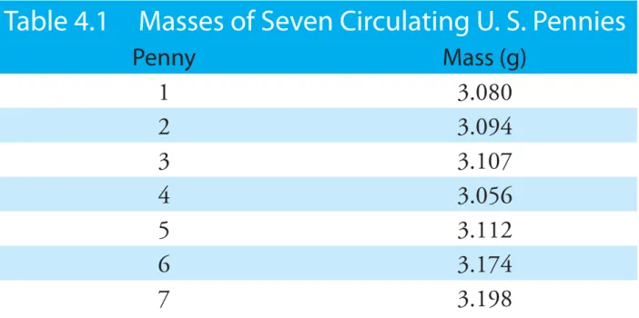
A good way to begin our analysis is to examine some preliminary data. Table 4.1 shows masses for seven pennies from my change jar. In
examin-ing this data it is immediately apparent that our question does not have a simple answer. That is, we can not use the mass of a single penny to draw a specific conclusion about the mass of any other penny (although we might conclude that all pennies weigh at least 3 g). We can, however, character-ize this data by reporting the spread of individual measurements around a central value.
4A.1 Measures of Central Tendency
One way to characterize the data in Table 4.1 is to assume that the masses are randomly scattered around a central value that provides the best esti-mate of a penny’s expected, or “true” mass. There are two common ways to estimate central tendency: the mean and the median.
MEAN
The mean, X , is the numerical average for a data set. We calculate the mean by dividing the sum of the individual values by the size of the data set
Figure 4.1 An uncirculated 2005 Lincoln head penny. The “D” be-low the date indicates that this penny was produced at the United States Mint at Denver, Colorado. Pennies produced at the Philadel-phia Mint do not have a letter be-low the date. Source: United States Mint image (www.usmint.gov).
Table 4.1 Masses of Seven Circulating U. S. Pennies
Penny Mass (g) 1 3.080 2 3.094 3 3.107 4 3.056 5 3.112 6 3.174 7 3.198
X X n i i =
∑
where Xi is the ith measurement, and n is the size of the data set.
Example 4.1
What is the mean for the data in Table 4.1?
S
OLUTIONTo calculate the mean we add together the results for all measurements 3.080 + 3.094 + 3.107 + 3.056 + 3.112 + 3.174 + 3.198 = 21.821 g and divide by the number of measurements
X = 21 821 = 7 3 117 . . g g
The mean is the most common estimator of central tendency. It is not a robust estimator, however, because an extreme value—one much larger or much smaller than the remainder of the data—strongly influences the mean’s value.1 For example, if we mistakenly record the third penny’s mass as 31.07 g instead of 3.107 g, the mean changes from 3.117 g to 7.112 g!
MEDIAN
The median, X% , is the middle value when we order our data from the smallest to the largest value. When the data set includes an odd number of entries, the median is the middle value. For an even number of entries, the median is the average of the n/2 and the (n/2) + 1 values, where n is the size of the data set.
Example 4.2
What is the median for the data in Table 4.1?
S
OLUTIONTo determine the median we order the measurements from the smallest to the largest value
3.056 3.080 3.094 3.107 3.112 3.174 3.198
Because there are seven measurements, the median is the fourth value in the ordered data set; thus, the median is 3.107 g.
As shown by Examples 4.1 and 4.2, the mean and the median provide similar estimates of central tendency when all measurements are compara-1 Rousseeuw, P. J. J. Chemom. 1991, 5, 1–20.
An estimator is robust if its value is not affected too much by an unusually large or unusually small measurement.
When n = 5, the median is the third value in the ordered data set; for n = 6, the me-dian is the average of the third and fourth members of the ordered data set.
ble in magnitude. The median, however, provides a more robust estimate of central tendency because it is less sensitive to measurements with extreme values. For example, introducing the transcription error discussed earlier for the mean changes the median’s value from 3.107 g to 3.112 g.
4A.2 Measures of Spread
If the mean or median provides an estimate of a penny’s expected mass, then the spread of individual measurements provides an estimate of the difference in mass among pennies or of the uncertainty in measuring mass with a balance. Although we often define spread relative to a specific mea-sure of central tendency, its magnitude is independent of the central value. Changing all measurements in the same direction, by adding or subtracting a constant value, changes the mean or median, but does not change the spread. There are three common measures of spread: the range, the standard deviation, and the variance.
RANGE
The range, w, is the difference between a data set’s largest and smallest values.
w = Xlargest – Xsmallest
The range provides information about the total variability in the data set, but does not provide any information about the distribution of individual values. The range for the data in Table 4.1 is
w = 3.198 g – 3.056 g = 0.142 g
STANDARD DEVIATION
The standard deviation, s, describes the spread of a data set’s individual values about its mean, and is given as
s X X n i i = − −
∑
( )2 1 4.1 where Xi is one of n individual values in the data set, and X is the data set’s mean value. Frequently, the relative standard deviation, sr, is reported.s s X r =
The percent relative standard deviation, %sr, is sr × 100.
Example 4.3
What are the standard deviation, the relative standard deviation and the percent relative standard deviation for the data in Table 4.1?
Problem 12 at the end of the chapter asks you to show that this is true.
S
OLUTIONTo calculate the standard deviation we first calculate the difference between each measurement and the mean value (3.117), square the resulting differ-ences, and add them together to give the numerator of equation 4.1.
( . . ) ( . ) . ( . . 3 080 3 117 0 037 0 001369 3 094 3 1 2 2 − = − = − 117 0 023 0 000529 3 107 3 117 0 2 2 2 ) ( . ) . ( . . ) ( . = − = − = − 0010 0 000100 3 056 3 117 0 061 0 0 2 2 2 ) . ( . . ) ( . ) . = − = − = 003721 3 112 3 117 0 005 0 000025 3 1 2 2 ( . . ) ( . ) . ( . − = − = 7 74 3 117 0 057 0 003249 3 198 3 117 2 2 − = + = − . ) ( . ) . ( . . )22 0 081 2 0 006561 0 015554 = +( . ) = . .
Next, we divide this sum of the squares by n – 1, where n is the number of measurements, and take the square root.
s = − = 0 015554 7 1 0 051 . . g
Finally, the relative standard deviation and percent relative standard devia-tion are sr g g = 0 051 = 3 117 0 016 . . . %sr = (0.016) × 100% = 1.6%
It is much easier to determine the standard deviation using a scientific calculator with built in statistical functions.
VARIANCE
Another common measure of spread is the square of the standard deviation, or the variance. We usually report a data set’s standard deviation, rather than its variance, because the mean value and the standard deviation have the same unit. As we will see shortly, the variance is a useful measure of spread because its values are additive.
Example 4.4
What is the variance for the data in Table 4.1?
S
OLUTIONThe variance is the square of the absolute standard deviation. Using the standard deviation from Example 4.3 gives the variance as
s2 = (0.051)2 = 0.0026
Many scientific calculators include two keys for calculating the standard deviation. One key calculates the standard deviation for a data set of n samples drawn from a larger collection of possible samples, which corresponds to equation 4.1. The other key calculates the standard deviation for all possible samples. The later is known as the population’s standard deviation, which we will cover later in this chapter. Your calculator’s manual will help you de-termine the appropriate key for each. For obvious reasons, the numerator of equation 4.1 is called a sum of squares.
4B Characterizing Experimental Errors
Characterizing the mass of a penny using the data in Table 4.1 suggests two questions. First, does our measure of central tendency agree with the penny’s expected mass? Second, why is there so much variability in the individual results? The first of these questions addresses the accuracy of our measurements, and the second asks about their precision. In this section we consider the types of experimental errors affecting accuracy and precision. 4B.1 Errors Affecting Accuracy
Accuracy is a measure of how close a measure of central tendency is to the expected value, μ. We can express accuracy as either an absolute error, e
e = X −μ 4.2
or as a percent relative error, %er.
%er X μ
μ
= − ×100 4.3
Although equations 4.2 and 4.3 use the mean as the measure of central tendency, we also can use the median.
We call errors affecting the accuracy of an analysis determinate. Al-though there may be several different sources of determinate error, each source has a specific magnitude and sign. Some sources of determinate error are positive and others are negative, and some are larger in magnitude and others are smaller. The cumulative effect of these determinate errors is a net positive or negative error in accuracy.
We assign determinate errors into four categories—sampling errors, method errors, measurement errors, and personal errors—each of which we consider in this section.
SAMPLING ERRORS
A determinate sampling error occurs when our sampling strategy does not provide a representative sample. For example, if you monitor the
envi-Practice Exercise 4.1
The following data were collected as part of a quality control study for the analysis of sodium in serum; results are concentrations of Na+ in mmol/L.
140 143 141 137 132 157 143 149 118 145 Report the mean, the median, the range, the standard deviation, and the variance for this data. This data is a portion of a larger data set from An-drew, D. F.; Herzberg, A. M. Data: A Collection of Problems for the Student and Research Worker, Springer-Verlag:New York, 1985, pp. 151–155. Click here to review your answer to this exercise.
The convention for representing statistical parameters is to use a Roman letter for a value calculated from experimental data, and a Greek letter for the corresponding expected value. For example, the experi-mentally determined mean is X , and its underlying expected value is μ. Likewise, the standard deviation by experiment is s, and the underlying expected value is σ.
It is possible, although unlikely, that the positive and negative determinate errors will offset each other, producing a result with no net error in accuracy.
ronmental quality of a lake by sampling a single location near a point source of pollution, such as an outlet for industrial effluent, then your results will be misleading. In determining the mass of a U. S. penny, our strategy for selecting pennies must ensure that we do not include pennies from other countries.
METHOD ERRORS
In any analysis the relationship between the signal and the absolute amount of analyte, nA, or the analyte’s concentration, CA, is
Stotal =k nA A +Smb 4.4 Stotal = k CA A +Smb 4.5 where kA is the method’s sensitivity for the analyte and Smb is the signal from the method blank. A determinate method error exists when our value for kA or Smb is invalid. For example, a method in which Stotal is the mass of a precipitate assumes that k is defined by a pure precipitate of known stoichiometry. If this assumption is not true, then the resulting determination of nA or CA is inaccurate. We can minimize a determinate error in kA by calibrating the method. A method error due to an interferent in the reagents is minimized by using a proper method blank.
MEASUREMENT ERRORS
The manufacturers of analytical instruments and equipment, such as glass-ware and balances, usually provide a statement of the item’s maximum measurement error, or tolerance. For example, a 10-mL volumetric pipet (Figure 4.2) has a tolerance of ±0.02 mL, which means that the pipet delivers an actual volume within the range 9.98–10.02 mL at a tempera-ture of 20 oC. Although we express this tolerance as a range, the error is determinate; thus, the pipet’s expected volume is a fixed value within the stated range.
Volumetric glassware is categorized into classes depending on its accu-racy. Class A glassware is manufactured to comply with tolerances specified by agencies such as the National Institute of Standards and Technology or the American Society for Testing and Materials. The tolerance level for Class A glassware is small enough that we normally can use it without cali-bration. The tolerance levels for Class B glassware are usually twice those for Class A glassware. Other types of volumetric glassware, such as beakers and graduated cylinders, are unsuitable for accurately measuring volumes.
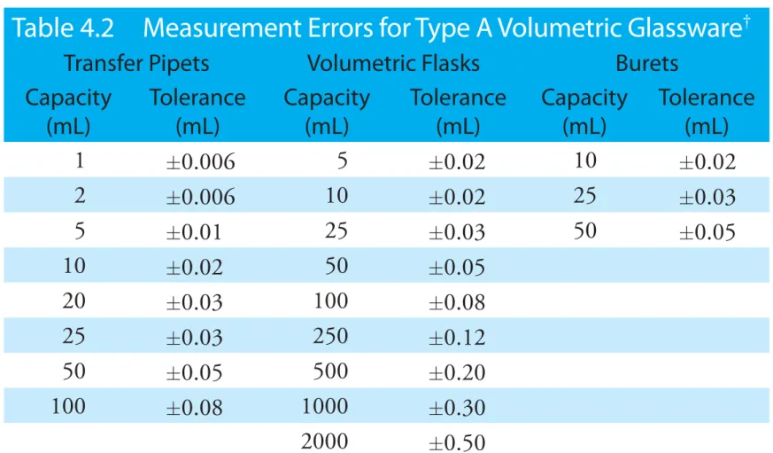
Table 4.2 provides a summary of typical measurement errors for Class A volumetric glassware. Tolerances for digital pipets and for balances are listed in Table 4.3 and Table 4.4.
We can minimize determinate measurement errors by calibrating our equipment. Balances are calibrated using a reference weight whose mass can
An awareness of potential sampling er-rors is especially important when working with heterogeneous materials. Strategies for obtaining representative samples are covered in Chapter 5.
Figure 4.2 Close-up of a 10-mL volumetric pipet showing that it has a tolerance of ±0.02 mL at 20 oC.
Table 4.2 Measurement Errors for Type A Volumetric Glassware
†Transfer Pipets Volumetric Flasks Burets Capacity (mL) Tolerance (mL) Capacity (mL) Tolerance (mL) Capacity (mL) Tolerance (mL) 1 ±0.006 5 ±0.02 10 ±0.02 2 ±0.006 10 ±0.02 25 ±0.03 5 ±0.01 25 ±0.03 50 ±0.05 10 ±0.02 50 ±0.05 20 ±0.03 100 ±0.08 25 ±0.03 250 ±0.12 50 ±0.05 500 ±0.20 100 ±0.08 1000 ±0.30 2000 ±0.50 †
Tolerance values are from the ASTM E288, E542, and E694 standards.
Table 4.3 Measurement Errors for Digital Pipets
†Pipet Range Volume (mL or μL)‡ Percent Measurement Error
10–100 μL 10 ±3.0% 50 ±1.0% 100 ±0.8% 100–1000 μL 100 ±3.0% 500 ±1.0% 1000 ±0.6% 1–10 mL 1 ±3.0% 5 ±0.8% 10 ±0.6% †
Values are from www.eppendorf.com. ‡ Units for volume match the units for the pipet’s range.
be traced back to the SI standard kilogram. Volumetric glassware and digi-tal pipets can be calibrated by determining the mass of water that it delivers or contains and using the density of water to calculate the actual volume. It is never safe to assume that a calibration will remain unchanged during an analysis or over time. One study, for example, found that repeatedly expos-ing volumetric glassware to higher temperatures durexpos-ing machine washexpos-ing and oven drying, leads to small, but significant changes in the glassware’s calibration.2 Many instruments drift out of calibration over time and may require frequent recalibration during an analysis.
2 Castanheira, I.; Batista, E.; Valente, A.; Dias, G.; Mora, M.; Pinto, L.; Costa, H. S. Food Control 2006, 17, 719–726.
PERSONAL ERRORS
Finally, analytical work is always subject to personal error, including the ability to see a change in the color of an indicator signaling the endpoint of a titration; biases, such as consistently overestimating or underestimating the value on an instrument’s readout scale; failing to calibrate instrumenta-tion; and misinterpreting procedural directions. You can minimize personal errors by taking proper care.
IDENTIFYING DETERMINATE ERRORS
Determinate errors can be difficult to detect. Without knowing the ex-pected value for an analysis, the usual situation in any analysis that matters, there is nothing to which we can compare our experimental result. Never-theless, there are strategies we can use to detect determinate errors.
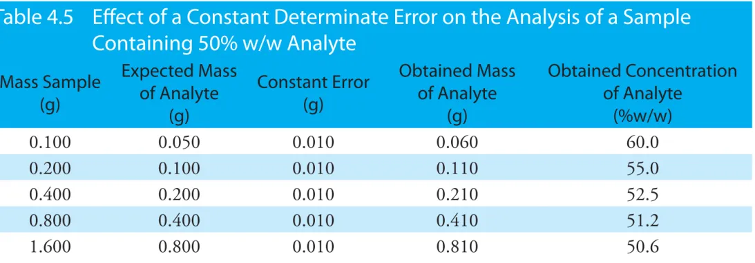
The magnitude of a constant determinate error is the same for all samples and is more significant when analyzing smaller samples. Analyzing samples of different sizes, therefore, allows us to detect a constant deter-minate error. For example, consider a quantitative analysis in which we separate the analyte from its matrix and determine its mass. Let’s assume that the sample is 50.0% w/w analyte. As shown in Table 4.5, the expected amount of analyte in a 0.100 g sample is 0.050 g. If the analysis has a positive constant determinate error of 0.010 g, then analyzing the sample gives 0.060 g of analyte, or a concentration of 60.0% w/w. As we increase the size of the sample the obtained results become closer to the expected result. An upward or downward trend in a graph of the analyte’s obtained
Table 4.4 Measurement Errors for Selected Balances
Balance Capacity (g) Measurement Error
Precisa 160M 160 ±1 mg
A & D ER 120M 120 ±0.1 mg
Metler H54 160 ±0.01 mg
Table 4.5 Effect of a Constant Determinate Error on the Analysis of a Sample
Containing 50% w/w Analyte
Mass Sample (g) Expected Mass of Analyte (g) Constant Error (g) Obtained Mass of Analyte (g) Obtained Concentration of Analyte (%w/w) 0.100 0.050 0.010 0.060 60.0 0.200 0.100 0.010 0.110 55.0 0.400 0.200 0.010 0.210 52.5 0.800 0.400 0.010 0.410 51.2 1.600 0.800 0.010 0.810 50.6concentration versus the sample’s mass (Figure 4.3) is evidence of a constant determinate error.
A proportional determinate error, in which the error’s magnitude depends on the amount of sample, is more difficult to detect because the result of the analysis is independent of the amount of sample. Table 4.6 outlines an example showing the effect of a positive proportional error of 1.0% on the analysis of a sample that is 50.0% w/w in analyte. Regardless of
the sample’s size, each analysis gives the same result of 50.5% w/w analyte. One approach for detecting a proportional determinate error is to ana-lyze a standard containing a known amount of analyte in a matrix similar to the samples. Standards are available from a variety of sources, such as the National Institute of Standards and Technology (where they are called standard reference materials) or the American Society for Testing and Materials. Table 4.7, for example, lists certified values for several analytes in a standard sample of Gingko bilboa leaves. Another approach is to compare your analysis to an analysis carried out using an independent analytical method known to give accurate results. If the two methods give signifi-cantly different results, then a determinate error is the likely cause.
Figure 4.3 Effect of a constant determinate error on the determi-nation of an analyte in samples of varying size.
Table 4.6 Effect of a Proportional Determinate Error on the Analysis of a Sample
Containing 50% w/w Analyte
Mass Sample (g) Expected Mass of Analyte (g) Proportional Error (%) Obtained Mass of Analyte (g) Obtained Concentration of Analyte (%w/w) 0.100 0.050 1.00 0.0505 50.5 0.200 0.100 1.00 0.101 50.5 0.400 0.200 1.00 0.202 50.5 0.800 0.400 1.00 0.404 50.5 1.600 0.800 1.00 0.808 50.5 Mass of Sample (g) Obtained C oncentration of Analyte (% w/w)Constant and proportional determinate errors have distinctly different sources, which we can define in terms of the relationship between the signal and the moles or concentration of analyte (equation 4.4 and equation 4.5). An invalid method blank, Smb, is a constant determinate error as it adds or
subtracts a constant value to the signal. A poorly calibrated method, which yields an invalid sensitivity for the analyte, kA, will result in a proportional determinate error.
4B.2 Errors Affecting Precision
Precision is a measure of the spread of individual measurements or results about a central value, which we express as a range, a standard deviation, or a variance. We make a distinction between two types of precision: repeat-ability and reproducibility. Repeatrepeat-ability is the precision when a single analyst completes the analysis in a single session using the same solutions, equipment, and instrumentation. Reproducibility, on the other hand, is the precision under any other set of conditions, including between analysts, or between laboratory sessions for a single analyst. Since reproducibility includes additional sources of variability, the reproducibility of an analysis cannot be better than its repeatability.
Errors affecting precision are indeterminate and are characterized by random variations in their magnitude and their direction. Because they are random, positive and negative indeterminate errors tend to cancel,
Table 4.7 Certified Concentrations for SRM 3246:
Ginkgo biloba
(Leaves)
†Class of Analyte Analyte Mass Fraction (mg/g or ng/g)
Flavonoids/Ginkgolide B Quercetin 2.69 ± 0.31
(mass fractions in mg/g) Kaempferol 3.02 ± 0.41
Isorhamnetin 0.517 ± 0.099
Total Aglycones 6.22 ± 0.77
Selected Terpenes Ginkgolide A 0.57 ± 0.28
(mass fractions in mg/g) Ginkgolide B 0.470 ± 0.090
Ginkgolide C 0.59 ± 0.22
Ginkgolide J 0.18 ± 0.10
Biloabalide 1.52 ± 0.40
Total Terpene Lactones 3.3 ± 1.1
Selected Toxic Elements Cadmium 20.8 ± 1.0
(mass fractions in ng/g) Lead 995 ± 30
Mercury 23.08 ± 0.17
†
The primary purpose of this Standard Reference Material is to validate analytical methods for determining flavonoids, terpene lactones, and toxic elements in Ginkgo biloba or other materials with a similar matrix. Values are from the official Certificate of Analysis available at www.nist.gov.
provided that enough measurements are made. In such situations the mean or median is largely unaffected by the precision of the analysis.
SOURCESOF INDETERMINATE ERROR
We can assign indeterminate errors to several sources, including collecting samples, manipulating samples during the analysis, and making measure-ments. When collecting a sample, for instance, only a small portion of the available material is taken, increasing the chance that small-scale inho-mogeneities in the sample will affect repeatability. Individual pennies, for example, may show variations from several sources, including the manu-facturing process, and the loss of small amounts of metal or the addition of dirt during circulation. These variations are sources of indeterminate sampling errors.
During an analysis there are many opportunities for introducing in-determinate method errors. If our method for determining the mass of a penny includes directions for cleaning them of dirt, then we must be careful to treat each penny in the same way. Cleaning some pennies more vigor-ously than others introduces an indeterminate method error.
Finally, any measuring device is subject to an indeterminate measure-ment error due to limitations in reading its scale. For example, a buret with scale divisions every 0.1 mL has an inherent indeterminate error of
±0.01–0.03 mL when we estimate the volume to the hundredth of a mil-liliter (Figure 4.4).
EVALUATING INDETERMINATE ERROR
An indeterminate error due to analytical equipment or instrumentation is generally easy to estimate by measuring the standard deviation for sev-eral replicate measurements, or by monitoring the signal’s fluctuations over time in the absence of analyte (Figure 4.5) and calculating the standard deviation. Other sources of indeterminate error, such as treating samples inconsistently, are more difficult to estimate.
30
31
Figure 4.4 Close-up of a buret showing the difficulty in estimat-ing volume. With scale divisions every 0.1 mL it is difficult to read the actual volume to better than
±0.01–0.03 mL. Time (s) Signal (arbitrar y units)
Figure 4.5 Background noise in an instrument showing the ran-dom fluctuations in the signal.
To evaluate the effect of indeterminate measurement error on our analy-sis of the mass of a circulating United States penny, we might make several determinations for the mass of a single penny (Table 4.8). The standard deviation for our original experiment (see Table 4.1) is 0.051 g, and it is 0.0024 g for the data in Table 4.8. The significantly better precision when determining the mass of a single penny suggests that the precision of our analysis is not limited by the balance. A more likely source of indeterminate error is a significant variability in the masses of individual pennies.
4B.3 Error and Uncertainty
Analytical chemists make a distinction between error and uncertainty.3 Er-ror is the difference between a single measurement or result and its ex-pected value. In other words, error is a measure of bias. As discussed earlier, we can divide error into determinate and indeterminate sources. Although we can correct for determinate errors, the indeterminate portion of the er-ror remains. With statistical significance testing, which is discussed later in this chapter, we can determine if our results show evidence of bias.
Uncertainty expresses the range of possible values for a measurement or result. Note that this definition of uncertainty is not the same as our definition of precision. We calculate precision from our experimental data, providing an estimate of indeterminate errors. Uncertainty accounts for all errors—both determinate and indeterminate—that might reasonably affect a measurement or result. Although we always try to correct determi-nate errors before beginning an analysis, the correction itself is subject to uncertainty.
Here is an example to help illustrate the difference between precision and uncertainty. Suppose you purchase a 10-mL Class A pipet from a labo-ratory supply company and use it without any additional calibration. The pipet’s tolerance of ±0.02 mL is its uncertainty because your best estimate of its expected volume is 10.00 mL ± 0.02 mL. This uncertainty is pri-marily determinate error. If you use the pipet to dispense several replicate portions of solution, the resulting standard deviation is the pipet’s precision.
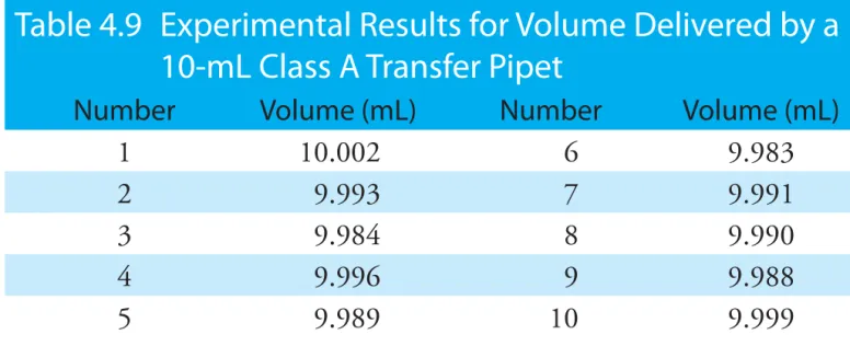
Table 4.9 shows results for ten such trials, with a mean of 9.992 mL and a standard deviation of ±0.006 mL. This standard deviation is the precision 3 Ellison, S.; Wegscheider, W.; Williams, A. Anal. Chem. 1997, 69, 607A–613A.
Table 4.8 Replicate Determinations of the Mass of a
Single Circulating U. S. Penny
Replicate Mass (g) Replicate Mass (g)
1 3.025 6 3.023
2 3.024 7 3.022
3 3.028 8 3.021
4 3.027 9 3.026
5 3.028 10 3.024
See Table 4.2 for the tolerance of a 10-mL class A transfer pipet.
In Section 4E we will discuss a statistical method—the F-test—that you can use to show that this difference is significant.
with which we expect to deliver a solution using a Class A 10-mL pipet. In this case the published uncertainty for the pipet (±0.02 mL) is worse than its experimentally determined precision (±0.006 ml). Interestingly, the data in Table 4.9 allows us to calibrate this specific pipet’s delivery volume as 9.992 mL. If we use this volume as a better estimate of this pipet’s ex-pected volume, then its uncertainty is ±0.006 mL. As expected, calibrating the pipet allows us to decrease its uncertainty.4
4C Propagation of Uncertainty
Suppose you dispense 20 mL of a reagent using the Class A 10-mL pipet whose calibration information is given in Table 4.9. If the volume and un-certainty for one use of the pipet is 9.992 ± 0.006 mL, what is the volume and uncertainty when we use the pipet twice?
As a first guess, we might simply add together the volume and the maximum uncertainty for each delivery; thus
(9.992 mL + 9.992 mL) ± (0.006 mL + 0.006 mL) = 19.984 ±0.012 mL It is easy to appreciate that combining uncertainties in this way overesti-mates the total uncertainty. Adding the uncertainty for the first delivery to that of the second delivery assumes that with each use the indeterminate error is in the same direction and is as large as possible. At the other ex-treme, we might assume that the uncertainty for one delivery is positive and the other is negative. If we subtract the maximum uncertainties for each delivery,
(9.992 mL + 9.992 mL) ± (0.006 mL − 0.006 mL) = 19.984 ± 0.000 mL we clearly underestimate the total uncertainty.
So what is the total uncertainty? From the previous discussion we know that the total uncertainty is greater than ±0.000 mL and less than ±0.012 mL. To estimate the cumulative effect of multiple uncertainties we use a mathematical technique known as the propagation of uncertainty. Our treatment of the propagation of uncertainty is based on a few simple rules.
4 Kadis, R. Talanta2004, 64, 167–173.
Table 4.9 Experimental Results for Volume Delivered by a
10-mL Class A Transfer Pipet
Number Volume (mL) Number Volume (mL)
1 10.002 6 9.983
2 9.993 7 9.991
3 9.984 8 9.990
4 9.996 9 9.988
5 9.989 10 9.999
Although we will not derive or further justify these rules here, you may consult the additional resources at the end of this chapter for references that discuss the propagation of uncertainty in more de-tail.
4C.1 A Few Symbols
A propagation of uncertainty allows us to estimate the uncertainty in a result from the uncertainties in the measurements used to calculate the result. For the equations in this section we represent the result with the symbol R, and the measurements with the symbols A, B, and C. The cor-responding uncertainties are uR, uA, uB, and uC. We can define the uncer-tainties for A, B, and C using standard deviations, ranges, or tolerances (or any other measure of uncertainty), as long as we use the same form for all measurements.
4C.2 Uncertainty When Adding or Subtracting
When adding or subtracting measurements we use their absolute uncertain-ties for a propagation of uncertainty. For example, if the result is given by the equation
R = A + B − C then the absolute uncertainty in R is
uR = uA2 +uB2 +uC2 4.6
Example 4.5
When dispensing 20 mL using a 10-mL Class A pipet, what is the total vol-ume dispensed and what is the uncertainty in this volvol-ume? First, complete the calculation using the manufacturer’s tolerance of 10.00 mL ± 0.02 mL, and then using the calibration data from Table 4.9.
S
OLUTIONTo calculate the total volume we simply add the volumes for each use of the pipet. When using the manufacturer’s values, the total volume is
V =10 00. mL+10 00. mL = 20 00. mL and when using the calibration data, the total volume is
V = 9 992. mL+9 992. mL =19 984. mL
Using the pipet’s tolerance value as an estimate of its uncertainty gives the uncertainty in the total volume as
uR = ( .0 02)2 +( .0 02)2 =0 028. mL
and using the standard deviation for the data in Table 4.9 gives an uncer-tainty of
uR = ( .0 006)2 +( .0 006)2 =0 0085. mL
The requirement that we express each un-certainty in the same way is a critically im-portant point. Suppose you have a range for one measurement, such as a pipet’s tolerance, and standard deviations for the other measurements. All is not lost. There are ways to convert a range to an estimate of the standard deviation. See Appendix 2 for more details.
Rounding the volumes to four significant figures gives 20.00 mL ± 0.03 mL when using the tolerance values, and 19.98 ± 0.01 mL when using the calibration data.
4C.3 Uncertainty When Multiplying or Dividing
When multiplying or dividing measurements we use their relative uncer-tainties for a propagation of uncertainty. For example, if the result is given by the equation
R A B C
= ×
then the relative uncertainty in R is R u A u B u C u R A B C 2 2 2 E O E O E O 4.7
Example 4.6
The quantity of charge, Q, in coulombs passing through an electrical cir-cuit is
Q = ×I t
where I is the current in amperes and t is the time in seconds. When a cur-rent of 0.15 A ± 0.01 A passes through the circuit for 120 s ± 1 s, what is the total charge passing through the circuit and its uncertainty?
S
OLUTIONThe total charge is
Q =( .0 15 A) (× 120 s)=18 C
Since charge is the product of current and time, the relative uncertainty in the charge is . . . R u 0 15 0 01 120 1 0 0672 R 2 2 F P E O
The absolute uncertainty in the charge is
uR = ×R 0 0672. =(18 C) ( .× 0 0672)=1 2. C Thus, we report the total charge as 18 C ± 1 C.
4C.4 Uncertainty for Mixed Operations
Many chemical calculations involve a combination of adding and subtract-ing, and multiply and dividing. As shown in the following example, we can calculate uncertainty by treating each operation separately using equation 4.6 and equation 4.7 as needed.
Example 4.7
For a concentration technique the relationship between the signal and the an analyte’s concentration is
Stotal =k CA A +Smb
What is the analyte’s concentration, CA, and its uncertainty if Stotal is 24.37 ± 0.02, Smb is 0.96 ± 0.02, and kA is 0.186 ± 0.003 ppm–1.
S
OLUTIONRearranging the equation and solving for CA
C S S k A total mb A ppm = − = 24 37−0 96− = 0 186 1 125 9 . . . . ppm
gives the analyte’s concentration as 126 ppm. To estimate the uncertainty in CA, we first determine the uncertainty for the numerator using equa-tion 4.6.
uR = ( .0 02)2 +( .0 02)2 = 0 028.
The numerator, therefore, is 23.41 ± 0.028. To complete the calculation we estimate the relative uncertainty in CA using equation 4.7.
. . . . . R u 23 41 0 028 0 186 0 003 0 0162 R 2 2 F P E O
The absolute uncertainty in the analyte’s concentration is uR =(125 9. ppm) ( .× 0 0162)= 2 0. ppm
Thus, we report the analyte’s concentration as 126 ppm ± 2 ppm.
Practice Exercise 4.2
To prepare a standard solution of Cu2+ you obtain a piece of copper from a spool of wire. The spool’s initial weight is 74.2991 g and its final weight is 73.3216 g. You place the sample of wire in a 500 mL volumetric flask, dissolve it in 10 mL of HNO3, and dilute to volume. Next, you pipet a 1 mL portion to a 250-mL volumetric flask and dilute to volume. What is the final concentration of Cu2+ in mg/L, and its uncertainty? Assume that the uncertainty in the balance is ±0.1 mg and that you are using Class A glassware.
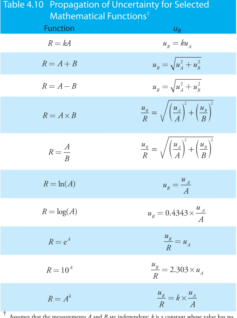
4C.5 Uncertainty for Other Mathematical Functions
Many other mathematical operations are common in analytical chemistry, including powers, roots, and logarithms. Table 4.10 provides equations for propagating uncertainty for some of these function.
Example 4.8
If the pH of a solution is 3.72 with an absolute uncertainty of ±0.03, what is the [H+] and its uncertainty?
Table 4.10 Propagation of Uncertainty for Selected
Mathematical Functions
† Function uR R =kA uR = kuA R = +A B uR = uA2 +uB2 R = A−B uR = uA2 +uB2 R = ×A B R u A u B u R A B 2 2 E O E O R A B = uRR uAA uBB 2 2 E O E O R = ln( )A u u A R A = R = log( )A u u A R A =0 4343. × R = eA u R u R A = R =10A u R u R A = 2 303. × R = Ak u R k u A R = × A †Assumes that the measurements A and B are independent; k is a constant whose value has no uncertainty.
S
OLUTIONThe concentration of H+ is
[ ] .
.
H+ =10−pH =10−3 72 =1 91 10× −4 M
or 1.9 ×10⁻⁴ M to two significant figures. From Table 4.10 the relative uncertainty in [H+] is u R u R A = 2 303. × = 2 303 0 03. × . = 0 069. The uncertainty in the concentration, therefore, is
( .1 91 10× −4 M)×( .0 069)=1 3 10. × −5 M We report the [H+] as 1.9 (±0.1) × 10–4 M.
4C.6 Is Calculating Uncertainty Actually Useful?
Given the effort it takes to calculate uncertainty, it is worth asking whether such calculations are useful. The short answer is, yes. Let’s consider three examples of how we can use a propagation of uncertainty to help guide the development of an analytical method.
One reason for completing a propagation of uncertainty is that we can compare our estimate of the uncertainty to that obtained experimentally. For example, to determine the mass of a penny we measure mass twice— once to tare the balance at 0.000 g, and once to measure the penny’s mass. If the uncertainty for measuring mass is ±0.001 g, then we estimate the uncertainty in measuring mass as
umass = ( .0 001)2 +( .0 001)2 =0 0014. g
Writing this result as
1.9 (±0.1) × 10–4 M is equivalent to
1.9 × 10⁻⁴ M ± 0.1 × 10⁻⁴ M
Practice Exercise 4.3
A solution of copper ions is blue because it absorbs yellow and orange light. Absorbance, A, is defined as
A P
P
=−log o
where Po is the power of radiation from the light source and P is the power after it passes through the solution. What is the absorbance if Po is 3.80×10² and P is 1.50×10²? If the uncertainty in measuring Po and P is 15, what is the uncertainty in the absorbance?
If we measure a penny’s mass several times and obtain a standard deviation of ±0.050 g, then we have evidence that our measurement process is out of control. Knowing this, we can identify and correct the problem.
We also can use propagation of uncertainty to help us decide how to improve an analytical method’s uncertainty. In Example 4.7, for instance, we calculated an analyte’s concentration as 126 ppm ± 2 ppm, which is a percent uncertainty of 1.6%. Suppose we want to decrease the percent un-certainty to no more than 0.8%. How might we accomplish this? Looking back at the calculation, we see that the concentration’s relative uncertainty is determined by the relative uncertainty in the measured signal (corrected for the reagent blank)
0 028
23 41 0 0012 .
. = . or 0.12%
and the relative uncertainty in the method’s sensitivity, kA, 0 003 0 186 0 016 1 1 . . . ppm ppm or 1.6% − − =
Of these terms, the uncertainty in the method’s sensitivity dominates the overall uncertainty. Improving the signal’s uncertainty will not improve the overall uncertainty of the analysis. To achieve an overall uncertainty of 0.8% we must improve the uncertainty in kA to ±0.0015 ppm–1.
Finally, we can use a propagation of uncertainty to determine which of several procedures provides the smallest uncertainty. When diluting a stock solution there are usually several different combinations of volumetric glassware that will give the same final concentration. For instance, we can dilute a stock solution by a factor of 10 using a 10-mL pipet and a 100-mL volumetric flask, or by using a 25-mL pipet and a 250-mL volumetric flask. We also can accomplish the same dilution in two steps using a 50-mL pipet
and 100-mL volumetric flask for the first dilution, and a 10-mL pipet and a 50-mL volumetric flask for the second dilution. The overall uncertainty in the final concentration—and, therefore, the best option for the dilution— depends on the uncertainty of the transfer pipets and volumetric flasks. As shown below, we can use the tolerance values for volumetric glassware to determine the optimum dilution strategy.5
5 Lam, R. B.; Isenhour, T. L. Anal. Chem. 1980, 52, 1158–1161.
Practice Exercise 4.4
Verify that an uncertainty of ±0.0015 ppm–1 for kA is the correct result. Click here to review your answer to this exercise.
2
100 1 6 ppm
126 ppm
Example 4.9
Which of the following methods for preparing a 0.0010 M solution from a 1.0 M stock solution provides the smallest overall uncertainty?
(a) A one-step dilution using a 1-mL pipet and a 1000-mL volumetric flask.
(b) A two-step dilution using a 20-mL pipet and a 1000-mL volumetric flask for the first dilution, and a 25-mL pipet and a 500-mL volumet-ric flask for the second dilution.
S
OLUTIONThe dilution calculations for case (a) and case (b) are case (a): 1.0 M 1.000 mL mL M c × = 1000 0. 0 0010. aase (b): 1.0 M 20.00 mL mL mL × × 1000 0 25 00 5 . . 0 00 0. mL =0 0010. M
Using tolerance values from Table 4.2, the relative uncertainty for case (a) is . . . . . R u 1 000 0 006 1000 0 0 3 0 006 R 2 2 E O E O
and for case (b) the relative uncertainty is
R uR 20 . 00 0 . 03 E O 2 1000 . 0 0 . 3 E O 2 25 . 00 0 . 03 F P 2 500 . 0 0 . 2 F P 2 0 . 002
Since the relative uncertainty for case (b) is less than that for case (a), the two-step dilution provides the smallest overall uncertainty.
4D The Distribution of Measurements and Results
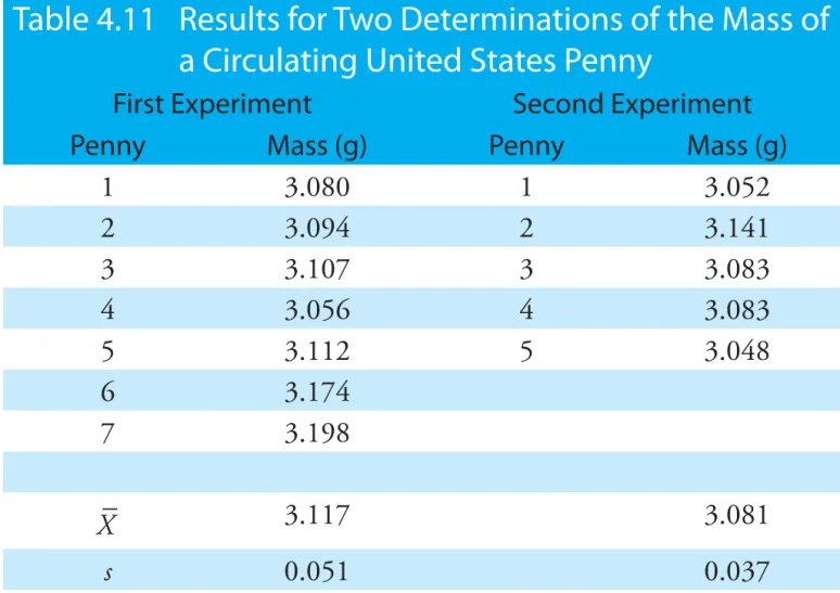
Earlier we reported results for a determination of the mass of a circulating United States penny, obtaining a mean of 3.117 g and a standard devia-tion of 0.051 g. Table 4.11 shows results for a second, independent deter-mination of a penny’s mass, as well as the data from the first experiment. Although the means and standard deviations for the two experiments are
similar, they are not identical. The difference between the experiments raises some interesting questions. Are the results for one experiment bet-ter than those for the other experiment? Do the two experiments provide equivalent estimates for the mean and the standard deviation? What is our best estimate of a penny’s expected mass? To answers these questions we need to understand how to predict the properties of all pennies by
analyz-See Appendix 2 for a more detailed treat-ment of the propagation of uncertainty.
ing a small sample of pennies. We begin by making a distinction between populations and samples.
4D.1 Populations and Samples
A population is the set of all objects in the system we are investigating. For our experiment, the population is all United States pennies in circulation. This population is so large that we cannot analyze every member of the
population. Instead, we select and analyze a limited subset, or sample of the population. The data in Table 4.11, for example, are results for two samples drawn from the larger population of all circulating United States pennies. 4D.2 Probability Distributions for Populations
Table 4.11 provides the mean and standard deviation for two samples of circulating United States pennies. What do these samples tell us about the population of pennies? What is the largest possible mass for a penny? What is the smallest possible mass? Are all masses equally probable, or are some masses more common?
To answer these questions we need to know something about how the masses of individual pennies are distributed around the population’s aver-age mass. We represent the distribution of a population by plotting the probability or frequency of obtaining an specific result as a function of the possible results. Such plots are called probability distributions.
There are many possible probability distributions. In fact, the probabil-ity distribution can take any shape depending on the nature of the popula-tion. Fortunately many chemical systems display one of several common probability distributions. Two of these distributions, the binomial distribu-tion and the normal distribudistribu-tion, are discussed in this secdistribu-tion.
Table 4.11 Results for Two Determinations of the Mass of
a Circulating United States Penny
First Experiment Second Experiment
Penny Mass (g) Penny Mass (g)
1 3.080 1 3.052 2 3.094 2 3.141 3 3.107 3 3.083 4 3.056 4 3.083 5 3.112 5 3.048 6 3.174 7 3.198 X 3.117 3.081 s 0.051 0.037
BINOMIAL DISTRIBUTION
The binomial distribution describes a population in which the result is the number of times a particular event occurs during a fixed number of trials. Mathematically, the binomial distribution is
P X N N X N X p p X N X ( , ) ! !( )! ( ) = − × × − − 1
where P(X , N) is the probability that an event occurs X times during N trials, and p is the event’s probability for a single trial. If you flip a coin five times, P(2,5) is the probability that the coin will turn up “heads” exactly twice.
A binomial distribution has well-defined measures of central tendency and spread. The expected mean value is
μ = Np
and the expected spread is given by the variance
σ2
1
= Np( − p) or the standard deviation.
σ = Np(1− p)
The binomial distribution describes a population whose members can take on only specific, discrete values. When you roll a die, for example, the possible values are 1, 2, 3, 4, 5, or 6. A roll of 3.45 is not possible. As shown in Example 4.10, one example of a chemical system obeying the binomial distribution is the probability of finding a particular isotope in a molecule.
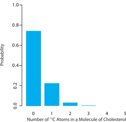
Example 4.10
Carbon has two stable, non-radioactive isotopes, 12C and 13C, with rela-tive isotopic abundances of, respecrela-tively, 98.89% and 1.11%.
(a) What are the mean and the standard deviation for the number of 13C atoms in a molecule of cholesterol (C27H44O)?
(b) What is the probability that a molecule of cholesterol has no atoms of 13C?
S
OLUTIONThe probability of finding an atom of 13C in a molecule of cholesterol follows a binomial distribution, where X is the number of 13C atoms, N is the number of carbon atoms in a molecule of cholesterol, and p is the probability that any single atom of carbon in 13C.
(a) The mean number of 13C atoms in a molecule of cholesterol is
The term N! reads as N-factorial and is the product N × (N-1) × (N-2) ×…× 1. For example, 4! is 4 × 3 × 2 × 1 = 24. Your calculator probably has a key for calculat-ing factorials.
μ = Np = 27 0 0111× . = 0 300. with a standard deviation of
σ= Np(1− p) = 27 0 0111× . ×(1 0 0111− . ) = 0 172.
(b) The probability of finding a molecule of cholesterol without an atom of 13C is P( , ) ! !( )! ( . ) ( . ) 0 27 27 0 27 0 0 0111 1 0 0111 0 27 = − × × − − −0 = 0 740.
There is a 74.0% probability that a molecule of cholesterol will not have an atom of 13C, a result consistent with the observation that the mean number of 13C atoms per molecule of cholesterol, 0.300, is less than one.
A portion of the binomial distribution for atoms of 13C in cholesterol is shown in Figure 4.6. Note in particular that there is little probability of finding more than two atoms of 13C in any molecule of cholesterol.
NORMAL DISTRIBUTION
A binomial distribution describes a population whose members have only certain, discrete values. This is the case with the number of 13C atoms in cholesterol. A molecule of cholesterol, for example, can have two 13C atoms, but it can not have 2.5 atoms of 13C. A population is continuous if its mem-bers may take on any value. The efficiency of extracting cholesterol from a sample, for example, can take on any value between 0% (no cholesterol extracted) and 100% (all cholesterol extracted).
The most common continuous distribution is the Gaussian, or normal distribution, the equation for which is
Figure 4.6 Portion of the bino-mial distribution for the number of naturally occurring 13C atoms in a molecule of cholesterol. Only 3.6% of cholesterol molecules contain more than one atom of
13
C, and only 0.33% contain
more than two atoms of 13C. 0. 0 1 2 3 4 5
0 0. 2 0.4 0.6 0.8 1.0 P robabilit y
f X X ( ) ( ) = − − 1 2 2 2 2 2 πσ σ e μ
where μ is the expected mean for a population with n members μ =
∑
X n
i i
and σ2 is the population’s variance.
σ2 2 = −
∑
(X ) n i i μ 4.8 Examples of normal distributions, each with an expected mean of 0 and with variances of 25, 100, or 400, are shown in Figure 4.7. Two features of these normal distribution curves deserve attention. First, note that each normal distribution has a single maximum corresponding to μ, and that the distribution is symmetrical about this value. Second, increasing the popula-tion’s variance increases the distribupopula-tion’s spread and decreases its height; the area under the curve, however, is the same for all three distribution.The area under a normal distribution curve is an important and useful property as it is equal to the probability of finding a member of the popula-tion with a particular range of values. In Figure 4.7, for example, 99.99% of the population shown in curve (a) have values of X between -20 and 20. For curve (c), 68.26% of the population’s members have values of X
between -20 and 20.
Because a normal distribution depends solely on μ and σ2, the prob-ability of finding a member of the population between any two limits is the same for all normally distributed populations. Figure 4.8, for example, shows that 68.26% of the members of a normal distribution have a value
Figure 4.7 Normal distribution curves for:
(a) μ= 0; σ2 = 25 (b) μ= 0; σ2 = 100 (c) μ= 0; σ2=400
within the range μ± 1σ, and that 95.44% of population’s members have values within the range μ± 2σ. Only 0.17% members of a population have values exceeding the expected mean by more than ± 3σ. Additional ranges and probabilities are gathered together in a probability table that you will find in Appendix 3. As shown in Example 4.11, if we know the mean and standard deviation for a normally distributed population, then we can de-termine the percentage of the population between any defined limits.
Example 4.11
The amount of aspirin in the analgesic tablets from a particular manu-facturer is known to follow a normal distribution with μ= 250 mg and
σ2= 25. In a random sampling of tablets from the production line, what percentage are expected to contain between 243 and 262 mg of aspirin?
S
OLUTIONWe do not determine directly the percentage of tablets between 243 mg and 262 mg of aspirin. Instead, we first find the percentage of tablets with less than 243 mg of aspirin and the percentage of tablets having more than 262 mg of aspirin. Subtracting these results from 100%, gives the
percent-age of tablets containing between 243 mg and 262 mg of aspirin.
To find the percentage of tablets with less than 243 mg of aspirin or more than 262 mg of aspirin we calculate the deviation, z, of each limit from μ
in terms of the population’s standard deviation, σ
z = X −μ
σ
where X is the limit in question. The deviation for the lower limit is
-3σ -2σ -1σ μ +1σ +2σ +3σ 34.13% 13.59 % 2.14 % 2.14 % 34.13% 13.59 % Value of X Figure 4.8 Normal distribution
curve showing the area under the curve for several different ranges of values of X. As shown here, 68.26% of the members of a nor-mally distributed population have values within ±1σ of the popula-tion’s expected mean, and 13.59% have values between μ–1σ and u–2σ. The area under the curve between any two limits can be found using the probability table in Appendix 3.
zlower = 243−250 =−
5 1 4.
and the deviation for the upper limit is
zupper = 262−250 = +
5 2 4.
Using the table in Appendix 3, we find that the percentage of tablets with less than 243 mg of aspirin is 8.08%, and the percentage of tablets with more than 262 mg of aspirin is 0.82%. Therefore, the percentage of tablets containing between 243 and 262 mg of aspirin is
100.00% - 8.08% - 0.82 % = 91.10%
Figure 4.9 shows the distribution of aspiring in the tablets, with the area in blue showing the percentage of tablets containing between 243 mg and 262 mg of aspirin.
230 240 250 260 270
Aspirin (mg) 8.08%
0.82%
91.10% Figure 4.9 Normal distribution
for the population of aspirin tab-lets in Example 4.11. The popula-tion’s mean and standard deviation are 250 mg and 5 mg, respectively. The shaded area shows the percent-age of tablets containing between 243 mg and 262 mg of aspirin.
Practice Exercise 4.5
What percentage of aspirin tablets will contain between 240 mg and 245 mg of aspirin if the population’s mean is 250 mg and the population’s standard deviation is 5 mg.
4D.3 Confidence Intervals for Populations
If we randomly select a single member from a population, what is its most likely value? This is an important question, and, in one form or another, it is at the heart of any analysis in which we wish to extrapolate from a sample to the sample’s parent population. One of the most important features of a population’s probability distribution is that it provides a way to answer this question.
Figure 4.8 shows that for a normal distribution, 68.26% of the popula-tion’s members are found within the range of μ± 1σ. Stating this another way, there is a 68.26% probability that the result for a single sample drawn from a normally distributed population is in the interval μ± 1σ. In general, if we select a single sample we expect its value, Xi to be in the range
Xi = ±μ zσ 4.9 where the value of z is how confident we are in assigning this range. Values reported in this fashion are called confidence intervals. Equation 4.9, for example, is the confidence interval for a single member of a population. Table 4.12 gives the confidence intervals for several values of z. For reasons
we will discuss later in the chapter, a 95% confidence level is a common choice in analytical chemistry.
Example 4.12
What is the 95% confidence interval for the amount of aspirin in a single analgesic tablet drawn from a population for which μ is 250 mg and σ2
is 25?
S
OLUTIONUsing Table 4.12, we find that z is 1.96 for a 95% confidence interval. Substituting this into equation 4.9, gives the confidence interval for a single tablet as
Xi= μ± 1.96σ= 250 mg ± (1.96 × 5) = 250 mg ± 10 mg When z = 1, we call this the 68.26%
con-fidence interval.
Table 4.12 Confidence Intervals for a
Normal Distribution (
μ
±
z
σ
)
z Confidence Interval (%) 0.50 38.30 1.00 68.26 1.50 86.64 1.96 95.00 2.00 95.44 2.50 98.76 3.00 99.73 3.50 99.95A confidence interval of 250 mg ± 10 mg means that 95% of the tablets in the population contain between 240 and 260 mg of aspirin.
Alternatively, we can express a confidence interval for the expected mean in terms of the population’s standard deviation and the value of a single member drawn from the population.
μ = Xi ± zσ 4.10
Example 4.13
The population standard deviation for the amount of aspirin in a batch of analgesic tablets is known to be 7 mg of aspirin. If you randomly select and analyze a single tablet and find that it contains 245 mg of aspirin, what is the 95% confidence interval for the population’s mean?
S
OLUTIONThe 95% confidence interval for the population mean is given as μ = Xi ±zσ= 245 mg±( .1 96 7× ) mg = 245 mg±14 mg
Therefore, there is 95% probability that the population’s mean, μ, lies within the range of 231 mg to 259 mg of aspirin.
It is unusual to predict the population’s expected mean from the analy-sis of a single sample. We can extend confidence intervals to include the mean of n samples drawn from a population of known σ. The standard deviation of the mean, σX , which also is known as the standard error of the mean, is
σX σ
n
=
The confidence interval for the population’s mean, therefore, is μ = ±X z
n
σ
4.11
Example 4.14
What is the 95% confidence interval for the analgesic tablets described in Example 4.13, if an analysis of five tablets yields a mean of 245 mg of aspirin?
S
OLUTIONIn this case the confidence interval is
Problem 8 at the end of the chapter asks you to derive this equation using a propa-gation of uncertainty.
μ = 245 mg±1 96 7× mg = mg± mg
5 245 6
.
Thus, there is a 95% probability that the population’s mean is between 239 to 251 mg of aspirin. As expected, the confidence interval when using the mean of five samples is smaller than that for a single sample.
4D.4 Probability Distributions for Samples
In working example 4.11–4.14 we assumed that the amount of aspirin in analgesic tablets is normally distributed. Without analyzing every member of the population, how can we justify this assumption? In situations where we can not study the whole population, or when we can not predict the mathematical form of a population’s probability distribution, we must de-duce the distribution from a limited sampling of its members.
SAMPLE DISTRIBUTIONS ANDTHE CENTRAL LIMIT THEOREM
Let’s return to the problem of determining a penny’s mass to explore further the relationship between a population’s distribution and the distribution of a sample drawn from that population. The two sets of data in Table 4.11
are too small to provide a useful picture of a sample’s distribution. To gain a better picture of the distribution of pennies we need a larger sample, such as that shown in Table 4.13. The mean and the standard deviation for this sample of 100 pennies are 3.095 g and 0.0346 g, respectively.
A histogram (Figure 4.10) is a useful way to examine the data in Table 4.13. To create the histogram, we divide the sample into mass intervals
and determine the percentage of pennies within each interval (Table 4.14). Note that the sample’s mean is the midpoint of the histogram.
Figure 4.10 also includes a normal distribution curve for the population of pennies, assuming that the mean and variance for the sample provide ap-propriate estimates for the mean and variance of the population. Although the histogram is not perfectly symmetric, it provides a good approximation of the normal distribution curve, suggesting that the sample of 100 pennies
Practice Exercise 4.6
An analysis of seven aspirin tablets from a population known to have a standard deviation of 5, gives the following results in mg aspirin per tablet:
246 249 255 251 251 247 250
What is the 95% confidence interval for the population’s expected mean?
Table 4.13 Masses for a Sample of 100 Circulating U. S. Pennies
Penny Mass (g) Penny Mass (g) Penny Mass (g) Penny Mass (g)
1 3.126 26 3.073 51 3.101 76 3.086 2 3.140 27 3.084 52 3.049 77 3.123 3 3.092 28 3.148 53 3.082 78 3.115 4 3.095 29 3.047 54 3.142 79 3.055 5 3.080 30 3.121 55 3.082 80 3.057 6 3.065 31 3.116 56 3.066 81 3.097 7 3.117 32 3.005 57 3.128 82 3.066 8 3.034 33 3.115 58 3.112 83 3.113 9 3.126 34 3.103 59 3.085 84 3.102 10 3.057 35 3.086 60 3.086 85 3.033 11 3.053 36 3.103 61 3.084 86 3.112 12 3.099 37 3.049 62 3.104 87 3.103 13 3.065 38 2.998 63 3.107 88 3.198 14 3.059 39 3.063 64 3.093 89 3.103 15 3.068 40 3.055 65 3.126 90 3.126 16 3.060 41 3.181 66 3.138 91 3.111 17 3.078 42 3.108 67 3.131 92 3.126 18 3.125 43 3.114 68 3.120 93 3.052 19 3.090 44 3.121 69 3.100 94 3.113 20 3.100 45 3.105 70 3.099 95 3.085 21 3.055 46 3.078 71 3.097 96 3.117 22 3.105 47 3.147 72 3.091 97 3.142 23 3.063 48 3.104 73 3.077 98 3.031 24 3.083 49 3.146 74 3.178 99 3.083 25 3.065 50 3.095 75 3.054 100 3.104
Table 4.14 Frequency Distribution for the Data in Table 4.13
Mass Interval Frequency (as %) Mass Interval Frequency (as %)
2.991–3.009 2 3.104–3.123 19 3.010–3.028 0 3.124–3.142 12 3.029–3.047 4 3.143–3.161 3 3.048–3.066 19 3.162–3.180 1 3.067–3.085 15 3.181–3.199 2 3.086–3.104 23
is normally distributed. It is easy to imagine that the histogram will more closely approximate a normal distribution if we include additional pennies in our sample.
We will not offer a formal proof that the sample of pennies in Table 4.13 and the population of all circulating U. S. pennies are normally distributed. The evidence we have seen, however, strongly suggests that this is true.
Al-though we can not claim that the results for all analytical experiments are normally distributed, in most cases the data we collect in the laboratory are, in fact, drawn from a normally distributed population. According to the central limit theorem, when a system is subject to a variety of in-determinate errors, the results approximate a normal distribution.6 As the number of sources of indeterminate error increases, the results more closely approximate a normal distribution. The central limit theorem holds true even if the individual sources of indeterminate error are not normally dis-tributed. The chief limitation to the central limit theorem is that the sources of indeterminate error must be independent and of similar magnitude so that no one source of error dominates the final distribution.
An additional feature of the central limit theorem is that a distribu-tion of means for samples drawn from a populadistribu-tion with any distribudistribu-tion will closely approximate a normal distribution if the size of the samples is large enough. Figure 4.11 shows the distribution for two samples of 10 000 drawn from a uniform distribution in which every value between 0 and 1 occurs with an equal frequency. For samples of size n = 1, the resulting dis-tribution closely approximates the population’s uniform disdis-tribution. The distribution of the means for samples of size n = 10, however, closely ap-proximates a normal distribution.
6 Mark, H.; Workman, J. Spectroscopy1988, 3, 44–48.
2.95 3.00 3.05 3.10 3.15 3.20 3.25 Mass of Pennies (g)
Figure 4.10 The blue bars show a histogram for the data in Table 4.13. The height of a bar corre-sponds to the percentage of pennies within the mass intervals shown in Table 4.14. Superimposed on the histogram is a normal distribution curve assuming that μ and σ2 for the population are equivalent to
X and s2 for the sample. The total area of the histogram’s bars and the area under the normal distribution curve are equal.
You might reasonably ask whether this aspect of the central limit theorem is im-portant as it is unlikely that we will com-plete 10 000 analyses, each of which is the average of 10 individual trials. This is deceiving. When we acquire a sample for analysis—a sample of soil, for example— it consists of many individual particles, each of which is an individual sample of the soil. Our analysis of the gross sample, therefore, is the mean for this large num-ber of individual soil particles. Because of this, the central limit theorem is relevant.
DEGREES OF FREEDOM
In reading to this point, did you notice the differences between the equa-tions for the standard deviation or variance of a population and the stan-dard deviation or variance of a sample? If not, here are the two equations:
σ2 2 = −
∑
(X ) n i i μ s X X n i i 2 2 1 = − −∑
( )Both equations measure the variance around the mean, using μ for a popu-lation and X for a sample. Although the equations use different measures for the mean, the intention is the same for both the sample and the popula-tion. A more interesting difference is between the denominators of the two equations. In calculating the population’s variance we divide the numera-tor by the population’s size, n. For the sample’s variance we divide by n – 1, where n is the size of the sample. Why do we make this distinction?
A variance is the average squared deviation of individual results from the mean. In calculating an average we divide by the number of indepen-dent measurements, also known as the degrees of freedom, contributing to the calculation. For the population’s variance, the degrees of freedom is equal to the total number of members, n, in the population. In measuring
Figure 4.11 Histograms for (a) 10 000 samples of size n = 1 drawn from a uniform distribution with a minimum value of 0 and a maximum value of 1, and (b) the means for 10 000 samples of size n = 10 drawn from the same uniform distribution. For (a) the mean of the 10 000 samples is 0.5042, and for (b) the mean of the 10 000 samples is 0.5006. Note that for (a) the distribution closely approximates a uniform distribution in which every possible result is equally likely, and that for (b) the distribution closely approximates a normal distribution.
0.2 0.3 0.4 0.5 0.6 0.7 0.8 0 500 1000 1500 2000 0.0 0.2 0.4 0.6 0.8 1.0 0 100 200 300 400 500
Value of X for Samples of Size n = 1 Value of X for Samples of Size n = 10
_ (a) (b) F requenc y F requenc y d