Least Orthogonal Distance Estimator and Total Least Square for Simultaneous Equation Models

(1)

Dipartimento di Economia, Università di Roma Tre, Roma, Italia Davide Zurlo

ISTAT – Ististuto Nazionale di Statistica, Roma, Italia Luciano Pieraccini

Dipartimento di Economia, Università di Roma Tre, Roma, Italia

1. INTRODUCTION

As it is well known the relations between structural form (SF) and Reduced form (RF) parameters of simultaneous equation models are established in the so called identifying system of equations. These are nothing else but linear relations between variable affected by error once RF estimates are considered.

It may be worth to remember that T. W. Anderson (1976) in a very well known paper explicitly recognized it saying: “It turns out, however, that a problem investigated in great detail by econometricians can be transformed so that it is mathematically identical to the problem of fitting a straight line when both variables are subjected to error. In estimating a coefficient of an (endogenous) variable in one equation in a system of simultaneous equations, the first stage is to find the sample regression coefficients of the dependent (endogenous) variables on the independent (exogenous) variables. The sample regression coefficients are mathematically equivalent to the observations in the model described above, and the population regression coefficient satisfy a linear relationship”. Along this line of thought Limited Information (LI) LODE has been produced initially (Pieraccini 1983, 1988) while more recently a first version of FI LODE was developed (Pieraccini and Naccarato, 2008).

A new version of FI LODE is presented here based on a new structure of the variance-covariance matrix that is employed in the estimation process. While in the previous version FI LODE was based on the variance-covariance matrix of error components related to the whole system of identifying equation, in the present one the variance-covariance matrix only refers to the error component of the so called over identifying equations.

(2)

computational algorithm based on SVD is numerically more robust with respect to the one based on SD; where robustness has to be understood as the greater probability to converge presented by the algorithm (Markovsky and Van Huffel 2007; Jennings 1980). In the light of these results a new computational procedure has been developed following the work of Gleser (1981) applying the Total Least Square procedure (Golub and Van Loan 1980; Van Huffel 1988, 1989, 2002, 2007).

The reason for the new version of FI LODE and for the use of a more robust estimation procedure has to be found in the results of a previous simulation experiment (Naccarato and Zurlo, 2008). The results showed that while FI LODE works usually better than other classic full information estimators in terms of bias, in terms of mean square error the estimates were affected by the presence of few very far outliers that weighted heavily on Mean Square Error (MSE).

A new Monte Carlo experiment (with the same structure of the one presented in the previous contribution) was then produced to evaluate the performance of the method with respect both to other classic full information methods and to the preceding FI LODE version.

In order to establish notation simultaneous equation models are briefly presented in paragraph 1 together with the original LI LODE, revisited in the light of SVD. In paragraph 2 the new version of FI LODE is shown and in paragraph 3 Total Least Square procedure is applied to. In paragraph 4 the complete design of the simulation experiment is presented. In paragraph 5 FILODE is compared with some usual methods of estimation like 3SLS (Theil and Zelner 1962) and FIML (Koopmans et al. 1950); the results are shown focusing on bias and MSE of estimators. In paragraph 6 few words of conclusion including a comparison between the previous version of FI LODE and the present one end the paper.

2. SIMULT

ANEOUS EQUATIONS SYSTEM

As it is well known the structural form (SF) of a simultaneous equation model can be defined as follows:

Γ +

Β +

=

, , , , ,

0

,

n m m m

Y

n k k m

X

n m

U

n m (1)

where Y is the n×m matrix of endogenous variables and Γ is the corresponding

m

m× matrix of structural parameters, X is the n×k matrix of exogenous variables and

Β

is the k×m matrix of their structural parameters. Finally U is the n×m ma-trix of disturbances with

=

= Ω ⊗

E(vec )

E[vec (vec ) ]

T

U

I

0

(2)

(3)



_σ







Ω =







_σ







2 1 1 2 1 m m m

⋯

⋮

⋱

⋮

⋯

is the constant variance-covariance matrix of the disturbances.

The reduced form (RF) of system (1), under non singularity condition for

Γ

, is

=

Π +

, , , ,

n m

Y

n k k m

X

V

n m (3)

where

−

Π = − Γ

= − Γ

1

, , ,

1

,

, ,

k m k m m m m m n m n m

V

U

B

(4)

As it is well known the first of (4) gives the link between RF and SF parameters which post-multiplied by

Γ

gives

Π Γ = −

, , ,

k m m m k m

B

₍₅₎

Introducing then exclusion conditions the following identification system for i-th equation is obtained:

ε



_{Π Γ +}

₌





Π Γ =





1 1 1 1 1

2 1 1

11 1 1 1

, ,1 ,

12 1 2 , ,1

ˆ

i

i i i k m m k m

i

i i k m m

B

(6) where:

π

−





Π =







1 1 1



11 01 11

, 1 ,1

ˆ

i

_ˆ

i

_ˆ

ie

k m k

⋮

refers to OLS estimates of reduced form parameters of endogenous and exogenous varia-bles included in the i-th equation;

π

−





Π =







2 2 2



12 02 12

, 1 ,1

ˆ

i

_ˆ

i

_ˆ

ie

k m k

⋮

(4)

var-iables’ coefficients included in the i-th equation; finally

ε

₁_i and

ε

₂_i are the error compo-nents of the system.

In the original paper in which the limited information version of LODE was proposed (Pieraccini 1988), the estimation was based on the second subsystem of (6) and not on the whole system as it was in the more recent paper (Pieraccini and Naccarato 2008). We have decided to go back to the original version of LODE and to derive the full infor-mation version starting from that point. As it will be seen in the conclusion (§ 6) the goodness of this choice has been somehow confirmed by the simulation experiment.

To simplify the exposition of the new version of FI LODE and the computational procedure let us now introduced LI LODE (Pieraccini 1988) in the light of SVD. It can be shown (Pieraccini 1969) that in the second of (6) it is

ε

2

=

2 1

T

i

R X U

i i i (7)

where

R

₂_i comes from

−













_

_

_

_

=





_

_

_

_





_

_

_

_









1 1 1 1 2

2 2 1 2 2

1 1 11 12

, , ,

, 2 21 22

, , ,

i i i i i

i ii ii

k k k k k k T

i i

k k i ii ii

k k k k k k

R

X X

R

(8)

so that it is

E(

ε

₂i

)

=

0

,

ε ε

=

σ

2

2 2 22

E(

i Ti

)

i

R

ii.

According to the Spectral Decomposition theorem LI LODE estimators of structural parameters

Γ

_i’s are based on the eigenvector corresponding to the minimum eigenvalue of variance-covariance matrix

Π

ˆ

₁₂i

R

₂₂−1_ii

Π

ˆ

₁₂i T.

Since

R

₂₂ii

= Λ

C C

T , with

C

and

Λ

the matrices of eigenvectors and eigenvalues of

22ii

R

, it is possible to define

= Λ

−

1 2 22

T i

Q

C

.

Premultiplying the elements of the second equation of (6) for

Q

₂₂_i it will become

ε

Π Γ =

22

ˆ

12 1 22 2

i

i i i i

Q

(9)

LI LODE method is based on the minimization , with respect to

Γ

₁_i, of the variance covariance matrix

Q

22i

ε

2i. Using singular value decomposition (9) becomes

Π = Λ

22

ˆ

12

i T

i

(5)

with

=



_



_

1

,

mi

S

…

S

_,

Λ =

(

λ

)

1

diag

,

i

m

…

_and

=



_



_

1

,

mi

D

…

D

if

λ

₁

≠

0.

i

m

An approximation of

Q

₂₂i

Π

ˆ

₁₂i denoted

(

Π

)

'

22

ˆ

12

i i

Q

is needed together with a vector

P

such that

(

₂₂

Π

ˆ

₁₂

)

' ₁

=

₀

i

i m

Q

P

(11)

According to Eckart and Young (1936), the best rank

m

₁i

−

1

approximation

(

22

Π

ˆ

12

)

' i i

Q

of

Q

₂₂i

Π

ˆ

₁₂i , is given by

(

Π

)

= Λ

'

22

ˆ

12

i T

i

Q

S D

where it is

(

λ

−

)

Λ =

'

diag

₁

,

₁ ₁

, 0

i

m and the minimal correction is

(

)

λ

= −

Π −

Π

=

1

2 '

22 12 22 12 ( ) 1

ˆ

min

i i

i i m

rank L m

Q

_F .

The solution of equation (11) is given by the

m

₁_i-th vector of the matrix

D

, called ₁

i

m

d

,

that belongs to

N Q

(

₂₂i

Π

ˆ

₁₂i

)

' (the null space of the approximation matrix).

The estimate of the parameters entering the i-th equation is the normalized right singular vector of

Q

₂₂_i

Π

ˆ

₁₂i , namely the eigenvector of the matrix

Π

ˆ

i₁₂'

Q

₂₂_i'

Q

₂₂_i

Π

ˆ

₁₂i , associated to the smallest eigenvalue of this latter matrix.

The estimates of structural parameters

Γ

₁_i for the i-th structural equation are defined as

ν

Γ = −

1 ₁

0

1 ˆ

i

i m

i

d

, where

ν

₀_i is the element of the characteristic vector associated with right hand side endogenous variable.

It has to be noticed that

(

Π

)

=

1

'

22

ˆ

12 i

0

i

i m

Q

d

and

(

Q

₂₂i

Π

ˆ

₁₂i

)

' represents the

(

m

1i

−

1 )

dimensional subspace spanned by the first

(

m

1i

−

1 )

principal axis that

minimize the sum of squares orthogonal distance between the observed points and the subspace itself.

3. THE NEW VERSION OF FI LODE

The second equation of system (6) for the whole system of equation can be written as

Π Γ = Ξ

12 1 , , ,

ˆ

r m

r z z m (12)

(6)

ε













Ξ =

_

_









21 , 2

0

r m m

⋯

⋮

⋱

⋮

⋯

and, once the dependent endogenous variable is chosen in each equation, the

Γ

₁ matrix can be written as

− −

−









Γ









Γ =

_

_





Γ









11 1 11 1,1 1 , 1 1,1

0

m m e m z m e m m

I

⋱

with =

=

∑

1

m i i

z

m

where

m

is the number of structural form’s equations. The identity

matrix

−

I

_m contains the

m

coefficients of the dependent endogenous variables and −

Γ

1 1 1,1 i e i m

is the matrix of the coefficients of the endogenous explanatory variables of i-th

equation after the normalization rule. Let:

π



_Π







Π =







_Π







1 1 02 12 12 , 02 12

ˆ

0

0 ˆ

₀

ˆ

0

e

r z

m me

⋱

=

∑

2

1

m i i

r

k

and

(

)

σ



















_Ξ



₌

























2

11 2211 1 221 1 221

2

1 22 1 22 22

2

1 22 1 22 22

vec

i i m m

T

i i ii ii im im

m m mi mi mm mm

R

E

R

⋯

⋮

⋱

⋮

⋯

⋮

⋱

⋮

⋯

(13)

(7)

−













=

























1 1 1 2

2 1 2 2

11 12

1

, ,

21 22

,

, ,

i j i j

ij ij k k k k T

i j

ij ij k k

k k k k

R

X X

R

i

X

and

X

j being the matrix of exogenous variables ordered according to exogenous

included and excluded variables in i-th and j-th structural equation.

It has to be stressed the difference between (13) and the variance-covariance matrix considered in the previous version of LI LODE (Pieraccini and Naccarato 2008).

4. TOTAL LEAST SQUARE PROCEDURE

Total Least Square procedure has been applied to equation (12) to estimate endogenous variables’ coefficients. Let it be

σ

















=

_

_

















2

11 2211 1 221 1 221

2

2 2 1 22 1 22 22

2

1 22 1 22 22

i i m m

T

i i ii ii im im

m m mi mi mm mm

R

Q Q

R

⋯

⋮

⋱

⋮

⋯

⋮

⋱

⋮

⋯

(14)

where

−

= Λ

1

2

T

Q

V

(15)

and

V

and

Λ

are – respectively – the matrix of eigenvectors (the first) and the diagonal matrix of eigenvalues of (14) (the second).

The endogenous variables parameters estimates are given by the matrix ₂

,

z m

D

of the last

m

singular right vectors that correspond to the

m

smallest singular values of

Q

₂

Π

ˆ

₁₂. According to Eckart and Young (1936) the best rank

z

−

m

matrix approximation of

Π

2

ˆ

12

Q

is defined as

(

Q

₂

Π

ˆ

₁₂

)

'

= Λ

S

'

D

T where

Λ =

'

diag

(

λ

₁

, ,

…

λ

_{z m}₋

, 0, , 0

…

)

_{is the}

singular values diagonal matrix of

Q

₂

Π

ˆ

₁₂ with the last

m

elements equal to zero.

S

and

D

are the left and right matrices of

Q

₂

Π

ˆ

₁₂, namely the respective eigenvectors of

(8)

( )= −

Π −

=

Π −

(

Π

)

=

_{= − +}

∑

λ

2 ' 2

2

2 12 2 12 2 12

1

ˆ

min

z i F

rank L z m _F

i z m

Q

L

Q

where

λ

i2 are the last

m

eigenvalues of

Π

ˆ

12 2 2

Π

ˆ

12

T

Q Q

.

Given the matrix D2 of the last

m

right singular vectors

−









=

_

_









12 , 2 , 22 , m m z m

z m m

D

, the equation

(

2

Π

12

)

' 2

=

,

ˆ

₀

r m

Q

D

is true.

Total Least Square procedure (Golub and Van Loan 1980; Van Huffel 2002) is then applied

( )

−









Γ





−

=

_

_







_Γ







1 11 1 1

2 12 1 1 1

ˆ

m e i m i im e m mi m

I

p

D

p

⋱

and the estimates of endogenous parameters for i-th equation are the sub-vector

Γ

ˆ

₁e_i of

( )

−

1

2 12

D D

.

The vector of the estimates of endogenous variables’ parameters

Γ

ˆ

₁ is



_Γ











Γ





Γ =













Γ













11 12 1 11 ,1 12 ,1 1 ,1 1 ,1

ˆ

m m m z m m

⋮

(16)

The exogenous coefficients matrix is then obtained as

(

)

−

(

)

Β =

ˆ

1 1 1 1 1 0

− Γ

1

ˆ

1

T T

X X

X

Y

(17)

where

X

₁ is the block diagonal matrix of exogenous variables included in each equation,

0

Y

is the left side endogenous variables vector’ for the m equations and

Y

1 is the right

side endogenous variables block diagonal matrix.

Equation (14) defines the matrix

Q

2 as a function of the elements

σ

2

ii and

σ

ij i.e. the

(9)

equations’ ones, which are both of them unknown. It is then necessary to estimate them. The disturbances variance-covariance matrix

Ω

ˆ

is obtained as in the previous version of FI LODE (Pieraccini and Naccarato 2008) through a two stage procedure.

Let

Γ

ˆ

₁_i be the first stage LI LODE estimates of the SF parameters and

V

ˆ

the matrix of RF equations’ residuals. Then the matrix of SF disturbances

U

ˆ

= − Γ

V

ˆ

is obtained in order to get

σ

− −

















Ω =

_

_

=

















2

11 1 1

1 1

2 2 2

1

2 1

ˆ

_ˆ

ˆ ˆ

ˆ

i m

T

i ii im

m mi mm

G U UG

⋯

⋮

⋱

⋮

⋯

⋮

⋱

⋮

⋯

(18) where −

























=

_

_

























1 1 2

1

0

1

0

1

0

i m

g

G

g

⋯

⋱

⋮

⋯

⋮

⋱

⋯

with

g

_i

= −

n

m

₁_i

−

k

₁_i. The second stage structural parameters estimates are then ob-tained introducing

σ

ˆ

in equation (15).

5. THE DESIGN OF THE EXPERIMENT

As in the previous simulation experiment (Naccarato and Zurlo, 2008), the new one has been performed using the three equation model proposed by Cragg in 1967:

= −

−

+





= −

+ +

+





_{= −}

_{+ +}

₊



1 2 3 2 5

2 1 3 5 7

3 2 3 4 6

0.89

0.16

44

0.74

0.13

0.74 62 0.70

0.96

0.06

0.29 40 0.53

0.11

0.56 y

y

x

y

x

y

x

(10)

sizes (let’s say with

n

=

1000

or even

n

=

10000

) on the ground that in the econometric practice the number of observations is generally not bigger than 30. Hence the following steps have been performed:

1. Exogenous variables generation. For each sample size exogenous variables have been generated from uniform distribution in the following intervals:

[

]

=

−

2

10 20

X

,

X

₃

=

[

15 27

−

]

,

X

₄

= −

[

3 12

]

,

X

₅

= −

[

3 7

]

,

[

]

=

−

6

20 50

X

,

X

₇

= −

[

7 13

]

.

Exogenous variables have been kept constant for each sample size.

2. Error component variance covariance matrix generation. The matrix

Ω

has been chosen in the following way:

a) diagonal elements have been obtained as a proportion of the variance of

Γ =

Y

Z

i.e.

ω

ii

=

σ

Z2

S

i

where

S

_i are proportionality coefficients randomly chosen from a uniform distribution in three intervals:

[

0.2 0.25

−

]

,

[

0.4 0.5

−

]

,

[

0.75 0.8

−

]

.

b) extra diagonal elements have been obtained at first generating randomly

(

−

1 2

)

m m

correlation coefficients

ρ

_ij in

[

0.1 0.2

−

]

,

[

0.4 0.5

−

]

,

[

0.8 0.9

−

]

assigning them a random sign. Then covariance between error

components in equation

i

and in equation

j

has been computed as

(

)

ω

=

ρ ω ω

12

ij ij ii jj _.

3. Normal and Uniform error distribution. For each sample of

n

observations,

m

series of random numbers have been generated independently from a standard-ized Normal distribution and from a Uniform distribution in the interval

(

−

3, 3

)

to have zero mean and variance one. To evaluate the performance of the estimation methods considered in non standard situation, the experiment has been extended to the case in which the error component is Uniformly dis-tributed in

(

−

10, 10

)

.

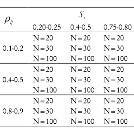
Table 1 shows the structure of the experiment as it was in Naccarato and Zurlo (2008). For each scenario 500 samples have been performed both for Normal and Uniform error components’ distribution.

To synthesize results of the simulation experiment two indicators have been considered: as it was in Naccarato and Zurlo (2008),

( )

ϕ θ θ θ

=

ˆ

−

₍₂₀₎

(11)

ψ

=

RMSE

θ

(21)

where RMSE is the Root Mean Square Error of

θ

ˆ

.

For both of them ratios between values presented by 3SLS and FIML with respect to FILODE are also computed.

TABLE 1 Simulation Scenarios

ρ

ij

S

i

0.20-0.25 0.4-0.5 0.75-0.80

0.1-0.2

N=20 N=20 N=20 N=30 N=30 N=30 N=100 N=100 N=100

0.4-0.5

N=20 N=20 N=20 N=30 N=30 N=30 N=100 N=100 N=100

0.8-0.9

N=20 N=20 N=20 N=30 N=30 N=30 N=100 N=100 N=100

6. RESULTS OF SIMULATION EXPERIMENT

Leaving to the next paragraph the comparison between the two versions of FI LODE we present here the results of the experiment with regard to the performance of FI LODE in the new version (using SVD) in comparison with that of two classical estimators like 3SLS and FIML.

We consider the results of the three methods first with regard to bias and then with regard to mean square error.

6.1.

Bias

As just pointed out, to evaluate the bias of the three methods under comparison we will make use of the indicator

ϕ

defined in (20). The analysis for the three situations foreseen with regard to error components, is separately presented.

Normal error component

(12)

With regard to average bias 16 times out of 27 FI LODE is performing better then FIML and 3SLS. Here too the situation improves for small samples (8 out of 9 cases) and increasing correlation.

To better compare the results, let’s consider Table 2 in which the ratios between average bias both of 3SLS and FIML with respect to FI LODE are presented.

FI LODE’s bias is very frequently smaller (values of the ratio greater than 1.05) or at most equal (values of the ratio between 0.95 and 1.05) to the one presented by FIML. It has to be stressed that this situation improves for small samples and increasing values of

ρ

. 3SLS always presents very high values of the ratio showing a very bad performance of the method with respect to average bias.

TABLE 2

Average bias ratio by

S

_i,

ρ

_i and sample size - Normal error component

ρ

i

0.1-0.2 0.4-0.5 0.8-0.9 FIML/ 3SLS/ FIML/ 3SLS/ FIML/ 3SLS/

i

S

_{Sample size FILODE FILODE FILODE FILODE FILODE FILODE} 0.2-0.25

20

1.42 5.97 2.16 3.19 1.92 5.74

0.4-0.5 3.88 2.21 2.66 7.00 1.72 0.71

0.75-0.8 0.76 1.42 1.68 2.19 4.82 1.91

0.2-0.25

30

1.18 6.64 0.97 8.72 1.03 12.55

0.4-0.5 1.08 5.48 0.42 4.00 14.16 7.00

0.75-0.8 0.85 5.98 6.21 10.86 23.71 13.62

0.2-0.25

100

0.68 25.46 0.57 21.85 0.95 30.21

0.4-0.5 0.96 14.18 0.50 11.19 0.40 9.40

0.75-0.8 0.57 21.85 1.14 23.49 1.21 24.11

Uniform error component

(

−

3, 3

)

When Uniform

(

−

3, 3

)

distribution of error component is considered results do not

change substantially, even if its percentage of lowest bias reduces to 13 times out of 27. Again FI LODE is almost always performing better then FIML for high values of

ρ

(in the interval

0.8 0.9

−

) and for small samples (

n

=

20, 30

). As before FILODE performs very much better then 3SLS whose bias is very high.

Uniform error component (-10, 10)

As we have already said, in order to evaluate the effect of non standard situation characterized by more scattered error components, a second Uniform distribution in the interval

(

−

10, 10

)

has been considered.

(13)

bias is largely lower than FIML’s one in most of the scenarios (Table 4). Moreover, it has to be noticed that FIML average bias is substantially bigger than the FILODE one even when

n

=

100

.

TABLE 3

S

_i,

ρ

_i and sample size - Uniform error component in

(

−

3, 3

)

ρ

i

S

Sample size FILODE FILODE FILODE FILODE FILODE FILODE

0.2-0.25

20

0.31 1.50 0.57 3.29 1.57 5.86

0.4-0.5 0.55 3.55 0.60 2.47 1.40 4.60

0.75-0.8 0.45 1.79 0.43 3.54 1.44 6.19

0.2-0.25

30

1.29 10.12 0.72 5.50 1.14 8.07

0.4-0.5 1.81 11.42 1.44 10.80 1.11 7.56

0.75-0.8 0.62 3.15 0.61 5.11 0.59 4.75

0.2-0.25

100

0.83 31.17 0.67 7.17 0.50 15.43

0.4-0.5 0.96 17.91 1.42 28.00 0.71 23.82

0.75-0.8 1.03 14.18 0.65 16.52 0.15 2.16

The average bias presented by 3SLS is almost everywhere bigger than the one presented by FI LODE with differences reaching 100%.

TABLE 4

S

_i,

ρ

(

−

10,10

)

ρ

i

S

20

2.74 2.00 1.53 1.13 0.69 1.09

0.4-0.5 1.66 1.06 1.14 1.52 1.01 1.08

0.75-0.8 5.32 0.85 2.71 1.29 1.02 0.98

0.2-0.25

30

14.36 1.81 1.44 1.98 1.71 1.21

0.4-0.5 8.29 0.82 2.90 1.20 6.60 1.00

0.75-0.8 9.25 1.24 2.73 1.16 2.47 0.97

0.2-0.25

100

200.32 1.38 221.66 1.00 88.75 1.79

0.4-0.5 288.59 1.11 421.31 1.13 316.46 1.30

(14)

6.2.

Mean Square Error

To evaluate the performance of the three methods with respect to RMSE we will make use of

ψ

defined in (21): relative frequency distribution of lowest values will be considered and the actual values presented. Here too, the ratio between RMSE both of 3SLS and FIML with respect to FILODE is given.

Normal error component

Looking at RMSE the situation is somehow different from the one seen for bias: The estimator that shows more frequently the lowest RMSE is FIML with 21 cases out of 27.

It has nevertheless to be noticed (Table 5) that when the differences between FIML and FI LODE are in favor of the first one they are almost always small and frequently less than or equal to 5%. As ever, FI LODE seems to work better for small samples and high correlation. Almost the same happens with regard to 3SLS that only sometimes performs better than FILODE.

TABLE 5

Average RMSE ratio by

S

_i,

ρ

i

S

20

1.28 1.24 0.92 1.10 1.19 1.22

0.4-0.5 1.03 0.36 1.95 1.08 3.87 0.90

0.75-0.8 0.69 0.54 0.33 0.39 0.98 0.28

0.2-0.25

30

1.00 1.11 0.79 1.02 0.75 1.06

0.4-0.5 1.46 0.92 0.57 0.63 7.64 1.03

0.75-0.8 1.02 0.97 1.91 0.55 1.86 0.51

0.2-0.25

100

0.95 1.21 0.84 1.11 0.75 1.43

0.4-0.5 0.97 1.21 0.95 1.22 0.70 1.16

0.75-0.8 0.98 1.14 0.83 1.19 0.71 1.30

(

−

3, 3

)

The results are very similar to those seen for Normal distribution.

(15)

(

−

10, 10

)

As far as estimators’ RMSE is concerned the comparison has to be made only between

TABLE 6

S

_i,

ρ

(

−

3, 3

)

ρ

i

S

20

0,81 0.90 0.79 1.07 0.64 0.59

0.4-0.5 0.78 0.75 0.61 0.85 0.70 0.57

0.75-0.8 0.63 0.66 0.53 0.65 0.62 0.84

0.2-0.25

30

0.95 1.11 0.77 1.02 0.74 0.68

0.4-0.5 0.99 1.04 0.97 1.03 0.74 0.65

0.75-0.8 0.69 0.61 0.44 0.65 0.53 0.82

0.2-0.25

100

0.97 1.08 0.90 1.02 0.79 0.65

0.4-0.5 0.96 1.15 0.77 1.19 0.69 0.59

0.75-0.8 0.93 1.11 1.04 1.24 0.53 0.62

LODE and 3SLS, since FIML estimators always produce higher RMSE than the other two methods. In general 3SLS is the one that presents the lowest RMSE, in accordance with what is established in literature. Only in few cases FI LODE performs better than 3SLS.

TABLE 7

S

_i,

ρ

(

−

10, 10

)

ρ

i

S

20

7.31 1.28 2.20 0.86 2.75 0.63

0.4-0.5 5.40 0.89 1.40 0.58 2.24 0.76

0.75-0.8 7.16 0.73 4.83 0.63 5.11 0.54

0.2-0.25

30

8.38 0.48 2.02 0.49 4.49 0.49

0.4-0.5 10.71 0.47 2.56 0.44 12.68 0.42

0.75-0.8 15.45 0.42 4.25 0.37 6.44 0.48

0.2-0.25

100

1212.57 1.05 826.84 0.43 154.21 0.48

0.4-0.5 1018.79 0.34 491.36 0.31 579.59 0.52

(16)

While with respect to FIML the ratio between RMSE (Table 7) is showing a very strong prevalence of FI LODE, with respect to 3SLS the situation is almost everywhere in favour of the last one even if with very much smaller differences.

7. CONCLUSION

In this work we present a LODE estimator inspired by Gleser (1981) and by the Total Least Square procedure introduced by Golub and Van Loan (1980) and Van Huffel (2002), in which estimates of structural form parameters is obtained using the last m smallest singular right vectors associated to the m smallest singular values. The performances of this estimator are very good both in terms of bias and RMSE. In particular has to be notice that it works better than 3SLS and FIML in case of small samples and high correlation. A quite substantial improvements of the performances of FI LODE is shown in standard situation like the one considered in the Monte Carlo experiment presented here.

Few general considerations about LODE’s performance can be made:

1) with regard to bias it can be said that LODE seems to perform better than the other two methods with which it is compared with. Both for Normal and Uniform distribution, LODE’s bias seems to be lower than FIML almost for all scenarios; it has in particular to be stressed its good performances for small samples and increasing correlation. The same happens with 3SLS which almost in all the situations present a bias greater than FILODE

2) similar consideration can be made with regard to RMSE even if the good performance of FI LODE is a little less stringent than in the preceding case. In particular it has to be stressed its very good performance for Uniform

(

−

10, 10

)

errors’ distribution if compared with FIML estimator which

performs quite badly. It is not the same with 3SLS average RMSE which is almost everywhere the lowest one.

From these considerations it seems to appear that FI LODE performs at least as well as FIML both with respect to bias and to mean square error. With the very strong exception of the case of Uniform distribution in (-10,10) in which the latter is out-performed by the former.

If compared with 3SLS, FI LODE performs always better both for bias and mean square error. Only exception is the better performance of the first one with regard to RMSE in the case of Uniform

(

−

10, 10

)

.

Let’s now go back to the many times postponed comparison between the two versions of FILODE: the one proposed in (Pieraccini and Naccarato 2008): and the one presented here. The first one is based on SD of the errors’ variance-covariance matrix related to the whole system of identifying equations, while the second one is based on SVD of errors’ variance-covariance matrix related only to over identifying equations, The comparison will then take into account both the difference between variance-covariance matrices considered in the two version and the computational procedure applied (SVD and SD).

(17)

2008 and 2nd_{Version the current one.}

As ever, relative frequency distribution of lowest values will be considered and the actual values presented. Here too, the ratio between bias and mean square error of the two versions will be given.

In terms of bias the 2nd_Version_{of FI LODE presents the best results 19 times out of}

27 with respect to the previous version of FI LODE, frequently with very high percentages.

TABLE 8

S

_i,

ρ

i

0.1-0.2 0.4-0.5 0.8-0.9

i

S

Sample size

1 2

st nd

1 2

st nd

1 2

st nd 0.2-0.25

20

2.00 1.90 2.25

0.4-0.5 0.53 1.63 0.31

0.75-0.8 0.59 0.77 1.04

0.2-0.25

30

5.00 2.50 4.33

0.4-0.5 2.67 1.85 1.64

0.75-0.8 1.67 3.67 5.33

0.2-0.25

100

3.67 2.75 7.75

0.4-0.5 3.17 7.00 4.83

0.75-0.8 5.80 11.33 7.00

TABLE 9

S

_i,

ρ

i

0.1-0.2 0.4-0.5 0.8-0.9

i

S

Sample size

1 2

st nd

1 2

st nd

1 2

st nd 0.2-0.25

20

1.36 1.19 1.11

0.4-0.5 _0.39 _1.25 _1.02

0.75-0.8 _1.01 _0.42 _0.39

0.2-0.25

30

1.31 1.22 1.03

0.4-0.5 _1.34 _0.76 _1.14

0.75-0.8 _1.43 _0.83 _0.64

0.2-0.25

100

1.11 1.11 1.32

0.4-0.5 _1.36 _1.28 _1.03

(18)

The average bias of 2nd_Version_{of FILODE is almost everywhere lower than the other}

one (Table 8) sometimes presenting a very high value of the ratio (especially for

n

=

20

) showing a very strong reduction of the bias. A generalized improvement of the new version with respect to bias has then to be recognized.

Also with regard to RMSE the 2nd_Version_{of FILODE presents a generalized}

improvement: here too 19 times out of 27 it is the one with the lowest average (Table 9); the ratio between average RMSE of the two versions is almost every time in favor of the new one.

From these consideration it becomes evident that the 2nd_Version_{of FI LODE presents a}

strong improvement with respect to the preceding one.

REFERENCES

T. W. ANDERSON (1976). Estimation of linear functional relationship: approximate distribution and connections with simultaneous equation in econometrics. Journal of the Royal Statistics Society, series B, 38, pp. 1-20.

J.G.CRAGG (1967). On Relative Small Sample Properties of Several Structural Equation Estimator. Econometrica, 35.

C.ECKART,G.YOUNG (1936). The approximation of one matrix by another of lower rank. Psychometrika, 1, no. 3.

L.GLESER, (1981). Estimation in a multivariate “errors in variable model” regression model:

Large sample results. Ann. Statistics, 9, pp. 525-534.

G.H.GOLUB,C.VAN LOAN (1980). An analysis of the total least square problem. SIAM J., Number Anal. 17.

L.S.JENNINGS (1980). Simultaneous Equation Estimation computational aspects. Journal of Econometrics, 12, pp. 23-39.

T. C. KOOPMANS,H.RUBIN,R.B. LEIPNIK (1950). Measuring the Equation System of Dynamic Economics. In Statistical Inference in Dynamic Economic Models, T. C. Koopmans (eds.), New York John Wiley & Sons, Inc., Chapter 2, pp. 53-237.

I.MARKOVSKY,S.VAN HUFFEL (2007). Overview on total least square. Signal Processing, 87, pp. 2283-2303.

A.NACCARATO,D.ZURLO (2008). A Monte Carlo Study on Full Information Methods in Simultaneous Equation Models. Quaderni di Statistica, 10, pp. 115-144.

L. PIERACCINI, A. NACCARATO (2008). Full information Least Orthogonal Distance

(19)

L. PIERACCINI (1988). Il metodo L.O.D.E. per la stima dei parametri strutturali di un sistema di equazioni simultanee. Quaderni di statistica e Econometria, X, pp. 5-14.

L.PIERACCINI (1983). The Estimation of Structural Parameters in Simultaneous Equation Models. Quaderni di statistica e Econometria, V, pp. 1-21.

L.PIERACCINI (1969). Su un’interpretazione alternativa del metodo dei minimi quadrati a

due stadi. Statistica, 4 XI, pp. 786-802.

H. THEIL, A. ZELLNER (1962). Three stage least squares: simultaneous estimation of simultaneous equation. Econometrica, 30.

S.VAN HUFFEL (2007). Total least square and error in variable model. Computational Statistics and Data Analysis, 52, pp. 1076-1079.

S.VAN HUFFEL (2002). Total Least Squares and Errors-In-Variables Modeling: Analysis, Algorithms and Applications. Kluwer Academic Publications.

S.VAN HUFFEL (1989). The partial total least square algorithm. J. Computational Analysis, 93, pp. 149-162.

S.VAN HUFFEL (1988). Analysis an properties of the generalized total least square problem. SIAM J., Matrix Anal. Appl., 10, pp. 294-315.

SUMMARY

Least Orthogonal Distance Estimator and Total Least Square for Simultaneous Equation Models