IMAGE REGISTRATION BASED ON MAXIMIZATION OF GRADIENT CODE MUTUAL INFORMATION

IMAGE REGISTRATION BASED ON MAXIMIZATION OF GRADIENT

CODE MUTUAL INFORMATION

X

W

J

T

Medical Image Processing Group, Key Laboratory of Complex Systems and Intelligence Science, Institute of Automation, Chinese Academy of Science, P.O.Box 2728, Beijing, 100080, China

e-mail: [email protected] (Accepted Jannuary 4, 2005)

ABSTRACT

Herein one proposes a mutual information-based registration method using pixel gradient information rather than pixel intensity information. Special care is paid to finding the global maximum of the registration function. In particular, one uses simulated annealing method speeded up by including a statistical analysis to reduce the next search space across the cooling schedule. An additional speed up is obtained by combining this numerical strategy with hill-climbing method. Experimental results obtained on a limited database of biological images illustrate that the proposed method for image registration is relatively fast, and performs well as the overlap between the floating and reference images is decreased and/or the image resolution is coarsened.

Keywords: gradient code mutual information, hill-climbing, image registration, mutual information, simulated annealing.

INTRODUCTION

Image registration is the process of aligning two or more images. A variety of approaches have been published. Good surveys are available in Maintz and Viergever (1998) and in Hajnal et al. (2001). Over the last few years, mutual information (MI) has become one of the most popular methods of image registration because it is more flexible and accurate than any other method based on global information content. However, MI method has its own limitations. For example, when the images are of low resolution, when the images contain little information, or when the region of overlap is small, MI may result in misregistration (Pluim et al., 2000a).

Since the initial work of Wells et al. (1996) and Maes et al. (1997), several groups have modified the optimization objective MI itself. It is worth mentioning Studholme et al. (1999) who introduced normalized MI to rigidly register multi-modal images with different fields of view, Pluim et al. (2000a) who added a gradient-based term to the MI function in order to decrease the number of local maxima, and Rueckert et al. (2000) who applied second order entropy estimation to model the dependency of a voxel gray

value on the intensities of a local neighborhood around that voxel. Other groups discussed registration with image features. Rangarajan et al. (1999) discussed feature point registration with MI. Hellier and Barillot (2003) coupled dense and landmark-based approaches for non-rigid registration. Johnson and Christensen (2002) used landmark and intensity information together to produce consistent correspondences between images. Hartkens et al. (2002) introduced feature information into voxel-based registration algorithms in order to incorporate higher-level information about the expected deformation. Butz and Thiran (2001; 2002) recalled the very general definition of MI and chose the feature of edgeness to perform image registration. These methods combining directly image features with MI have many advantageous properties of both feature-based and intensity-based methods. Our own work continues along this line.

annealing (SA), and then combine it with the local optimization of hill-climbing properly to reduce the number of iterations.

The remainder of this paper is organized as follows. Firstly, the method of GCMI is introduced. Then, the advantages of GCMI method are experimen-tally illustrated through applications to multimodal medical image registration. Finally, conclusions are provided.

METHOD

GRADIENT CODE

Take two 2D discrete images f(x,y) and r(x,y) to be registered. From f and r, we construct gradient code images, fg and rg, such that each pixel of the

images represents a gradient code that is, the quantification of gradient vector at the corresponding pixel position in the original gray-level images. Take f(x,y) as an example, the horizontal and vertical derivatives of f(x,y) are represented respectively as

x f f_x =∂ ∂

∇ / and ∇f_y =∂f /∂y. Partial differentials are calculated using central differences (Rosefeld and Kak, 1982). To avoid a reduction in image size, forward / backward differences are used for border pixels. Then the module (ρ_i,j) and the phase (θ_i,j) of the gradient vector (∇f_x,∇f_y) at a pixel (i,j) are calculated respectively as:

2 2

,j x y

i

=

∇

f

+

∇

f

ρ

α

θ

,j y x

i f f , (1)

If

∇

f

≠

0

∇

f

=

0

&

∇

f

≠

0

where α=0 if ∇f_x ≥0,∇f_y ≥0; α=π if ∇f_x<0; π

α =2 if ∇f_x >0,∇f_y <0.

Herein, for convenience purposes, we make the range ρ_i,j to be [0,1]. Then, the gradient code is obtained by dividingθ into N (=2π/∆_θ) level-intervals of constant width ∆_θ, and ρ into M (=1/∆_ρ) level-intervals of constant length ∆_ρ. We have to choose appropriate interval-sizes for precise registration of different modal images. This issue should be considered in relation to inherent information amount and spatial resolution. The gradient code (fg and rg

images) is ultimately defined as:

    

Γ > ∆

+ −

∆ =

otherwise L

if N

C

j i j

i j

i

j i, ,

,

,

] [ * ) ]

([ρ δ θ ρ

θ

ρ , (2)

where

   

= ∆ − ∆ =

otherwise if

0

0 ] [

1 i,j i,j

ρ ρ ρ ρ

δ ,

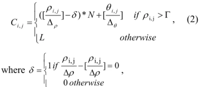
[x] represents the integer which is equal or less than x, Γ is a pre-specified threshold level for ignoring low contrast pixels coded as L (L is a large value). The purpose for using Γ is to prevent uniform or semi-uniform regions from influencing the MI evaluation as pixels with low contrast neighborhoods are more sensitive to noise. Using a too large value for Γ can cause the suppression of information in low contrast images. An example of the 2D gradient code is depicted in Fig. 1 for ∆_θ =π/4 and ∆_ρ =1/4.

Fig. 1. An example of 2D Gradient Code (∆_θ =π/4 and ∆_ρ =1/4).

The method can be easily extended to 3D discrete images. Similarly, we represent the gradient vector

) , ,

(∇f_x ∇f_y ∇f_z in spherical coordinates as:

2 2 2

,

,jk x y z

i

=

∇

f

+

∇

f

+

∇

f

ρ

) / (

cos 1 _,,

,

,jk z i jk

i f

ρ

θ

α

ϕ

,

,jk y x

i f f ,

If

∇

f

≠

0

∇

f

=

0

&

∇

f

≠

0

Then, the gradient code images are obtained by segmenting ρ into M (=1/∆_ρ) discrete level-intervals of constant width ∆_ρ, θ into N (=π/∆_θ ) intervals of width∆_θ, and φ into K (=2π/∆_ϕ) intervals of width

ϕ

         > ∆ + ∆ + − ∆ = otherwise L T if K K N

C ijk

k j i k j i k j i k j i ] [ * ] [ * * ) ] ([ , , , , , , , , , , ρ ϕ θ δ ρ ϕ θ ρ . (4)

GRADIENT CODE MI (GCMI)

MI is a widely used information theoretical distance measure between probability densities. The MI between two images f and r is:

) , ( ) ( )

(f H r H f r H

MI = + −

) | ( ) ( ) | ( )

(f H f r H r H r f

H − = −

= (5)

Where H( f) and H( r) stands for the entropies of images f and r, H( f,r) for their joint entropy, and

) | (f r

H , H(r| f) for the conditional entropies. Usually we use the generalized distance between joint probability distribution pfr ( f,r) and marginal probability

distributions pf (f ) and pr(r) to estimate the MI:

∑

=

r

f f r

fr fr r p f p r f p r f p MI , ( ) ( ) ) , ( log ) ,

( . (6)

Registration of the images f andrcan be defined as finding the geometrical transformation T (mapping the floating image f to the reference one r) which maximizes the MI registration measure. In Wells et al. (1996), the measured features were simply the voxel intensities. In Rueckert et al. (2000), the sampling space was defined by the intensities of two neighbor voxels (i.e., a two-dimensional feature space). In Butz and Thiran (2002), edgeness was defined as the feature space to estimate the MI. In this paper, we restrict the discussion to a feature space represented by gradient code information. Because MI is evaluated based on gradient code images, we call our approach Gradient Code Mutual Information (GCMI).

In practice, MI cannot be computed exactly due to the sampled nature of the floating and reference images. One obvious problem is that the transformed position of a voxel will generally not coincide with a grid point of the reference image, such that the corresponding intensity is unknown. Partial volume (PV) interpolation, originally proposed by Collignon et al. (1995; 1998) and Maes et al. (1997), is specifically designed to update the joint histogram of two images. It has been found PV interpolation generally outperforms linear interpolation in terms of smoothness of the MI registration criterion. This study uses PV interpolation for both MI and GCMI.

OPTIMIZATION STRATEGY

An optimal optimization strategy should converge to the global extreme of an optimized function and also be fast. Several strategies available in the literature including genetic algorithm (Parker, 1997), Powel’s method (Press et al., 1992), amoeba (Press et al., 1992) and SA (Goffe et al., 1994) are compared. The genetic algorithm is a relatively robust strategy, but its convergence to the global extremum is slow; amoeba and Powel’s method are faster optimizers, but they frequently terminate in local extremes. SA is a global optimization method that distinguishes between different local optima. It is fast and is more robust (Čapek et al., 2001). Therefore, we apply here the Metropolis SA strategy (Metropolis et al., 1953), and modify it to adaptively adjust the search space for the transformation parameters of optimization. That is, before updating the annealing temperature, we statistically analyze the whole results (including the transformation parameter sets and their corresponding MI values) performed at current temperature to obtain the maximum (MImax) and minimum (MImin) of the

objective function, and then calculate the middle value (MImid):

MImid = (MImax – MImin)/2 + MImin. (7)

Among all the parameter vectors (geometrical transformation mapping the floating image to the reference image) at this temperature, only those of the corresponding MI value being above the middle MImid

are retained. Within all these retained vectors, we get the maximum and minimum of each parameter, and then assigned them respectively as upper bound (ub) and lower bound (lb) of the optimization parameters for the next search space. Thus the optimization process is greatly speeded up for avoiding many useless evaluations of the objective function. Since the algorithm makes very few assumptions about the function to be optimized, it is robust with respect to non-quadratic surfaces.

1. Pick a random point in the search space. 2. Consider all the neighbors of the current state. 3. Choose the neighbor with the best quality and

move to that state.

4. Repeat 2 thru 4 until all the neighboring states are of lower quality.

5. Return the current state as the solution state. The scheme does not only prevent the optimizing course from trapping in local extrema, but also saves a large number of iterations. The whole algorithm is implemented as follows:

Step 1: Transform the two original images to be registered into gradient code images.

Step 2: Initialize the cooling schedule (initial temperature T = 5.0, temperature reduction factor rt = 0.85) and the parameter values (initial transformation parameter set x, upper and lower bounds on search space lb and ub), where the temperature is initially set at a relatively high value, which allows a large range of possible perturbations. Compute MI(x).

Step 3: Pick a new set of transformation parameter set x’, and compute MI(x’).

Step 4: Calculate the difference between MI(x) and MI(x’). If MI(x’) > MI(x) the new parameter is accepted; otherwise, acceptance or rejection is determined by the Boltzmann probability given by

) ) ( ) ( exp(

'

T x MI x MI

p= − − where T is the temperature parameter of the SA.

Step 5: If the number n of evaluations of the objective function is more than a large predefined number or if the current MI value is not changed within four successive iterations, then go to step 6. Otherwise, adjust the upper (ub) and lower bounds (lb) as mentioned above and accordingly the next search range vm = ub–lb, decrease the temperature according to the cooling schedule T = T0•rt, and go

to step 3.

Step 6: Perform hill-climbing algorithm for optimal search.

RESULTS

To illustrate the performance of our method, we consider hereafter two different 2D registration problems: T1 magnetic resonance (T1-MR) to T2 magnetic resonance (T2-MR), and T1-MR to computed tomography (CT) and compare the results obtained

by MI and GCMI methods (with ∆_θ =π/8 and 8

/ 1 =

∆_ρ ). Our images are real data from Beijing Tiantan hospital and consist of pairs of CT and MR (T1 and T2) images of 6 patients. Each studied pair of images relates to the same patient.

Then, we evaluate the efficiency of our method for 2D and 3D registration by duplicating the original MR images.

The study was approved by the local ethic committee and consented by the patients after explaining the purpose of the study. All the experiments below are based on our medical image processing platform 3Dmed (Tian et al., 2003).

ACCURACY

• MR-T1 and T2

T1- and T2-MR images are multimodal in that different tissue characteristics are imaged. Yet, the structure in both images remains similar. Each pair of images comes from the same patient and the same scan, and we assume accordingly that no transformation is required to align the images.

Fig. 2 displays the registration function of the T1-MR image to the T2-T1-MR image using GCMI and MI for translation along the Ox axis. In the left column of

Fig. 2 (images with full resolution), both methods perform well. In the mid column (images sub-sampled by a factor of eight in each dimension) and in the right column (image-overlap changed to 60%), the MI registration does not perform well, and the optimum is stretched and shifted. In contrast, the GCMI registration performs well and the optimum is accurately identified. The results illustrate that GCMI function is invariant to the reduced overlap between the floating and reference images and less sensitive to the sub-sampling rate.

• MR-T2 and CT

Fig. 2. T1- to T2-MR registration using GCMI and MI for translation along Ox axis. From left to right: images with full resolution, images sub-sampled by a factor of 8 in each dimension, and image-overlap changed to 60%.

Fig. 3. MR-CT registration using GCMI and MI. From left to right: images with full resolution for translation along Ox axis, image-overlap changed to 60% for rotation around Oz axis, and in addition images sub-sampled by a factor of 4 in each dimension for translation along Ox axis.

Table 1. Mean time requirement of three optimization methods for the registration of a pair of 2D images.

Method ∆θ z

[°] x

∆ [mm]

y

∆ [mm]

Total time [s]

Number of Iteration

Standard SA 1.117 0.712 0.655 1651 1801

Improved SA 0.011 0.038 0.010 455 496

Improved SA +

hill-climbing 0.006 0.012 0.041 66 72

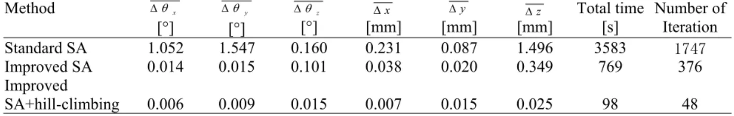
Table 2. Mean time requirement of three optimization methods for the registration of a pair of 3D images.

Method ∆θ x

[°]

y θ ∆

[°]

z θ ∆

[°] x

∆ [mm]

y

∆

[mm] [mm]∆z

Total time [s]

Number of Iteration

Standard SA 1.052 1.547 0.160 0.231 0.087 1.496 3583 1747

Improved SA 0.014 0.015 0.101 0.038 0.020 0.349 769 376

Improved

(a) (b) (c)

(d1) (d2) (d3) (d4)

(e1) (e2) (e3) (e4)

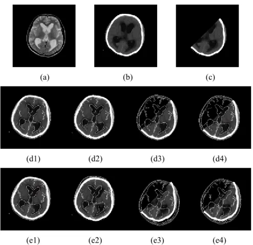
Fig. 4. Illustration of MR-CT registration results based on GCMI and MI. (a) MR floating image. (b) CT reference image. (c) Image containing 60% of the information in (b). From (d1) to (d4), GCMI registration results with full resolution images (d1), with images sub-sampled by a factor of 8 in each dimension (d2), with images sampled by a factor of 4 in each dimension and overlap changed to 60% (d3), and with images sub-sampled by a factor of 8 in each dimension and overlap changed to 60% (d4). (e1) to (e4): Corresponding results using MI.

Some results for MR-CT registration are illustrated in Fig. 4. On these examples, we clearly observe that when the images are of low resolution or when the image-overlap is reduced, the MI results in mis-registration, whereas, the GCMI performs better.

TIME REQUIREMENT

To illustrate the speed-up (time-wise) allowed by our numerical strategy, we duplicate a 2D MR image of size 256×256 and then register it to its original. Repeated experiments of this type illustrate that the registration using standard SA optimization (Table 1; 1st line) requires about 1650 seconds. The improved SA optimization (Table 1, 2nd line) requires only about 455 seconds with the accuracy significantly improved. When combining the improved SA optimization with hill-climbing method (Table 1, 3rd line), an accuracy of the same order is still observed, and the time is significantly reduced. To 3D volume registration, we duplicated a 3D MR image of size 256 × 256 × 24 and registered it to its original. The results are listed

in Table 2. All the experiments were performed using MATLAB on a PIII800, 128M.

CONCLUSIONS

As in Pluim et al. (2000b), we can observe the local extrema in both MI and GCMI functions (Figs. 2, 3) brought with the PV interpolation. According to the optimization strategy mentioned above, sub-pixel registration accuracy can be obtained (Table 1, 2). Several aspects of the method shall be improved or further investigated: mention in the first place the robustness of GCMI. Also, experiments with images of lower intrinsic resolution such as PET and SPECT should be carried out. This will be dealt with in the future work.

ACKNOWLEDGMENTS

We thank Ying Liu for helpful suggestions and Beijing Tiantan Hospital for providing the datasets. This research is supported by the National Science Fund for Distinguished Young Scholars of China under Grant No. 60225008 and the Beijing Natural Science Foundation of China under Grant No. 4042024.

REFERENCES

Butz T, Thiran JP (2001). Affine registration with feature space mutual information. MICCAI 2001; Utrecht, 549-56.

Butz T, Thiran JP (2002). Feature-space mutual information for multi-modal signal processing, with application to medical image registration. EUSIPCO 2002; Toulouse; France, 3-10.

Čapek M, Mrož L, Wegenkittl R (2001). Robust and fast medical registration of 3D-multi-modality data sets. IFMBE 1:515-8.

Collignon A, Maes F, Delaere D, Vandermeulen D, Suetens P, Marchal G (1995). Automated multimodality medical image registration using information theory. IPMI 1995; Computational Imaging and Vision, Brest, France, 263-74.

Collignon A (1998). Multimodality medical image regi-stration by maximization of mutual information. PhD thesis, Catholic University of Leuven, Leuven, Belgium. Goffe WL, Ferrier GD, Rogers J (1994). Global optimization

of statistical functions with simulated annealing. J Econom 60(1/2):65-100.

Hajnal JV, Hill DLG, Hawkes DJ (2001). Medical image registration. The biomedical engineering series. CRC Press, 39-71 and 281-303.

Hartkens T, Hill DLG, Castellano-Smith AD, Hawkes DJ, Maurer Jr. CR, Martin AJ et al. (2002). Using points and surfaces to improve voxel-based non-rigid registration. MICCAI(2) 2002; Tokyo, Japan, 565-72.

Hellier P, Barillot C (2003). Coupling dense and landmark-based approaches for non rigid registration. IEEE Trans Med Imaging 22(2):217-27.

Johnson HJ, Christensen GE (2002). Consistent landmark and intensity-based image registration. IEEE Trans Med Imaging 21(5):450-61.

Maes F, Collignon A, Vandermeulen D, Marchal G, Suetens P (1997). Multimodality image registration by maximization of mutual information. IEEE Trans Med Imaging 16(2):187-98.

Maintz JBA, Viergever MA (1998). A survey of medical image registration. Med Image Anal 2(1):1-36. Metropolis N, Rosenbluth A, Rosenbluth M, Teller A,

Teller E (1953). Equation of state calculations by fast computing machines. J Chem Phys 21(6):1087-92. Parker JR (1997). Algorithms for image processing and

computer vision. New York: John Wiley & Sons, 357-86.

Pluim JPW, Maintz JBA, Viergever MA (2000a). Image registration by maximization of combined mutual information and gradient information. IEEE Trans Med Imaging 1935:452-61.

Pluim JPW, Maintz JBA, Viergever MA (2000b). Interpolation artefacts in mutual information-based image registration. Comput Vis Image Unders 77(2): 211-32. Press W H, Flannery BP, Teukolsky SA, Vetterling WT

(1992). Numerical recipes in C: The art of scientific computing. 2nd _{ed. Cambridge University, 394-455.} Rangarajan A, Chui H, Duncan JS (1999). Rigid point feature

registration using mutual information. Med Image Anal 3(4):425-40.

Rosefeld A, Kak AC (1982). Digital picture processing. 2nd edition, vol. 2. San Diego: Academic Press.

Rueckert D, Clarkson MJ, Hill DLG, Hawkes DJ (2000). Non-rigid registration using higher-order mutual information. Proceedings of SPIE Medical Imaging 2000; San Diego, CA, 438-47.

Russell S, Norvig P (1995). Artificial intelligence: A modern approach. Prentice-Hall, 111-5.

Studholme C, Hawkes DJ, Hill DLG (1999). An overlap invariant entropy measure of 3D medical image alignment. Pattern Recogn 32:71-86.

Tian J, He H, Zhao M, Li G, Ge X, Zhu F (2003). An integrated 3D medical image processing and analysis system. Proceedings of SPIE International Symposium BiOS 2003; San Jose, USA, 284-93.