c
Abdullah Ali Faruq
A thesis submitted to the School of Graduate Studies in partial fulfillment of the requirements for the degree of
Master of Science
Department of Computer Science
Memorial University of Newfoundland February 2017
To my beloved mother who inspired me in every step of my life. She always wished for my success, but couldn’t be with us to share the joy.
Terrain aided navigation (TAN) is a well-studied method to localize an autonomous underwater vehicle in the absence of GPS. Researchers have been exploring new im-provements; in particular Bachmayer and Claus have been incorporating terrain based navigation (glider TAN) into the Slocum gliders. To take full advantage of glider TAN, the glider path should favour areas of the ocean with uneven depth and unique features. This leads to a question of planning such an "interesting" path for the glider. In this thesis, we present an offline path planning algorithm that optimizes the distance under the maximum uncertainty constraint. A major part of our contribu-tion is developing a rating technique for evaluating the usefulness of an area of the ocean floor for reducing the uncertainty of the glider’s position. We include experi-mental results showing how the generated path varies with the maximum allowable uncertainty, based on the ocean elevation data of the Conception Bay near Holyrood, Newfoundland.
Acknowledgements
I would like to thank all the people who contributed to this thesis with their help, support and inspiration. First and foremost, I thank my thesis supervisor Dr. An-tonina Kolokolova for her excellent guidance and understanding. Her vast knowledge and experience helped me shape my work as a graduate student. I really appreciated the freedom she gave me to explore so many research directions. I am grateful to have the opportunity to work under her supervision.
I must thank my loving wife Shameema Anwar, who has always supported me and stood beside me during my struggles. She gave me the strength I needed to cope with the tragedies I faced in the past few years.
Last but not the least, I want to show gratitude to my parents for their uncon-ditional love and support. I may have lost them, but their guidance will help me in every step of my life.
Abstract
Acknowledgments i
Table of Contents iv
List of Tables v
List of Figures vii
1 Introduction 1
1.1 Slocum underwater glider . . . 2
1.2 Localization . . . 2
1.3 Glider localization . . . 5
1.4 Problem statement . . . 6
1.5 Related work . . . 7
1.5.1 Path planning approaches in the literature . . . 8
1.5.2 Addressing the safety and uncertainty in path planning . . . . 11
1.6 Thesis organization . . . 13
2 Background 14 2.1 Probabilities and distribution . . . 14
2.1.1 Normal distribution . . . 17
2.2 Glider Navigation . . . 20
2.2.1 Dead Reckoning . . . 21
2.2.2 Terrain-Aided Navigation . . . 22
2.2.2.1 DEM: Digital Elevation Model . . . 22
2.2.2.2 Particle filter . . . 23
2.2.3 Glider TAN algorithm . . . 26
3 Rating 29 3.1 Inspecting the contribution of depth variation . . . 29
3.1.1 Effectiveness of rating: a point vs an area . . . 33
3.2 Representing an area for rating . . . 36
3.3 Constructing the rating . . . 37
3.4 Implementation of the rating . . . 41
3.4.1 Rating computed on the Holyrood data . . . 43
3.4.1.1 Rating map: a visual representation of depth variation 46 3.4.2 Comparing the result of rating using Holyrood data . . . 49
3.4.2.1 Comparing rating with estimation from a particle filter 49 3.4.2.2 Comparing rating with the effectiveness of glider TAN 51 4 Interesting Path Planning 54 4.1 Shortest Path Problem . . . 55
4.1.1 Algorithm for shortest path problem . . . 55
4.1.1.1 A* Algorithm for path planning . . . 56
4.1.1.2 Heuristic admissibility . . . 57
4.2 Interesting Path Problem . . . 57
4.2.1 Algorithm for interesting path planning . . . 59
4.3.2 Computing path in G′ . . . . 64
4.3.3 Proof of optimality . . . 65
4.4 Implementation . . . 70
4.4.1 Interesting path between a pair of waypoints . . . 71
4.4.2 The impact of uncertainty constraint over interesting path . . 72
5 Conclusion 75 5.1 Summary . . . 75
5.2 Future work . . . 75
Bibliography 76
List of Tables
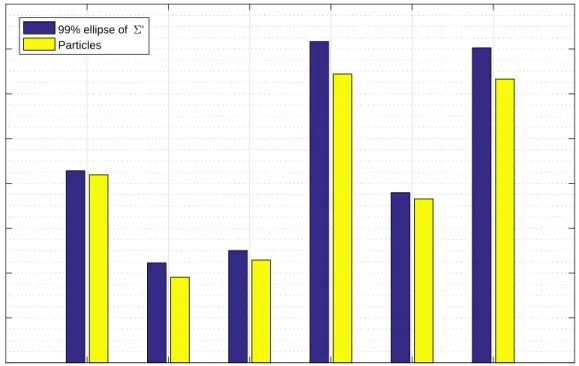
3.1 Comparing the rating result in different areas of the ocean near Holy-rood, NL using 99% confidence ellipse . . . 45 3.2 Comparing the result of rating calculation for the same area with
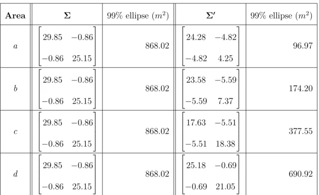
dif-ferent initial distribution varying in size, shape and rotation . . . 47 3.3 A comparison between the expected distribution from the rating
pro-cess and location estimation from particle filter simulation . . . 51
4.1 The impact of different uncertainty constraint in the resulted paths from the interesting path algorithm . . . 74
1.1 Autonomous underwater vehicle: a Slocum glider [cF05] . . . 3
2.1 Elevation of the ocean floor in Conception Bay near Holyrood, NL . . 24
3.1 The impact of depth variation on the particle cloud size . . . 32 3.2 Comparing the effectiveness of rating of a location and an area . . . . 35 3.3 Comparing the rating result in different areas of the ocean near
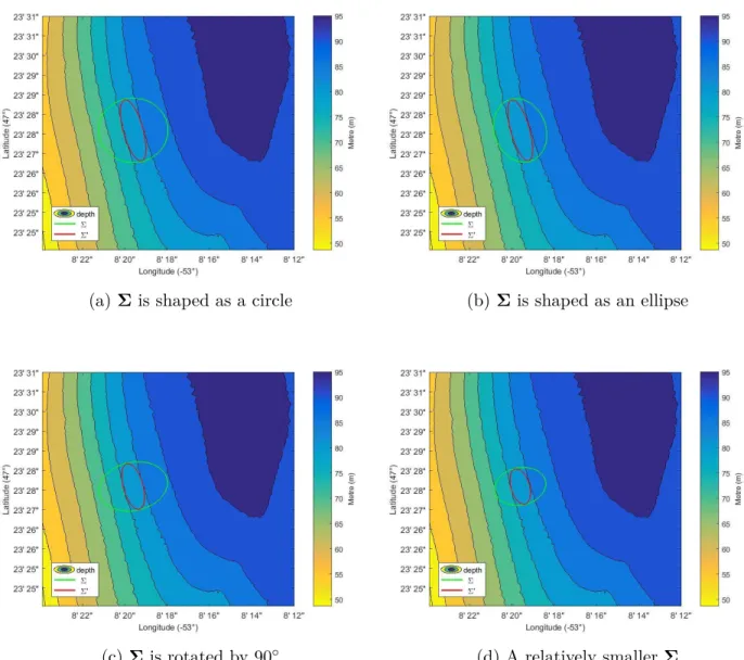
Holy-rood, NL using 99% confidence ellipse . . . 44 3.4 Comparing the result of rating calculation for the same area with
dif-ferent initial distribution varying in size, shape and rotation . . . 46 3.5 A visual representation of the rating of the entire region of the ocean
shown in Figure 2.1 using rating maps . . . 48 3.6 A comparison between the expected distribution from the rating
pro-cess and location estimation from particle filter simulation . . . 50 3.7 Comparing the rating estimation as a bound on the size of particle
cloud in glider TAN algorithm . . . 53
4.1 The comparison of edge traversal on an arbitrary edge (u, v)∈E . . . 60
4.2 Greedy algorithms like Dijkstra’s algorithm and A* can produce sub-optimal solution for interesting path problem . . . 61
4.3 The shortest path between the start and the goal locations bounded by the uncertainty constraint tmax = 38 meters . . . 71
4.4 Impact of different uncertainty constraints on the resulting paths from the interesting path algorithm . . . 73
Introduction
With the advancement in robotics, Autonomous Underwater Vehicles (AUVs) have gained rapid popularity in the past few decades. AUVs are capable of completing a variety of tasks without any active human assistance. In recent years, their capabilities and applications have grown significantly; specifically the Slocum glider is drawing
much attention in the research community. With a relatively slow speed, a glider can travel a long distance due to its low power consumption. Its long range capability along with economical value have encouraged its use in various underwater missions. Like any other AUV, a glider can suffer from inaccurate localization. In the absence of any GPS signal, a glider has to localize using information from the surrounding environment. Significant studies have been done on this area and researchers have developed many techniques to address the problem. But in an unpredictable and dynamic environment like an ocean, these techniques are not always enough. Back in 2013 a glider research team at Memorial University, lost a Slocum glider during a field trial near Holyrood, Newfoundland [New13]. Localization techniques such as terrain-aided navigation can help to improve glider localization, but to be able to localize more precisely, a glider needs to follow an "interesting" path that favours
2
certain areas in the ocean which are suitable for the on-board localization. Here, we are focusing our work on the quest of computing such interesting path for the glider. Although the finding of our work can be applied to other AUVs, we are specially interested in Slocum gliders.
1.1
Slocum underwater glider
Slocum gliders are relatively small AUVs with long range capabilities. These glid-ers use variable buoyancy engine to glide in a saw-tooth pattern. In the absences of an active propulsion system, they are comparatively slower than other AUVs. They are usually equipped with a number of sensors to measure the surrounding environ-ment. Here at the Autonomous Oceans Systems Lab of Memorial University, Dr. Ralf Bachmayer and Dr. Brian Claus have been working with Slocum gliders. They have performed multiple missions in the oceans near Newfoundland using these gliders. The primary motivation of our work came from the path planning requirements of those missions.
Despite their relatively slow speed, the gliders are well suited for a variety of missions including ocean data sampling and surveillance. Like any other autonomous vehicle, the mission success of a glider highly depends on its navigation capability, in particular on its localization technique.
1.2
Localization
In robotics, the term navigation refers to the task of safely and efficiently taking the robot from a given state to the desired state. In a simpler form, a state can be a point on a plane. In more complex cases, state includes location, orientation and other related information. The elements of a navigation system vary widely from one
Figure 1.1: Autonomous underwater vehicle: a Slocum glider [cF05]
design to another, but a fundamental part of most navigation is localization.
Localization is the process of acquiring knowledge about the current state of the robot in relation with its environment; in other words, knowing where the robot is actually located at a certain time. Usually it involves using a model of the environment or amap. The map can be constructed during the mission or a previously constructed
map may be available during the localization. The environment is perceived through a single or multiple sensors like a GPS, camera or range finder, each of which produces some form of information. Most localization methods use these acquired information to determine the current state of the robot relative to the map. This may sound simple, but in reality, it can become very challenging to get the current state with proper accuracy.
One major challenge of localization arises from the noise in sensor measurement. Most sensors produce slightly deviated value from the actual value in the environment. The magnitude of the deviation may vary depending on the type and quality of the sensor, but such deviation can occur in all sensors. Even the most sophisticated
4
sensor can be erroneous to some extent. Some of these errors can be corrected by calibrating the sensing device, but we can not eliminate the error completely. When these measurements are used to generate a map of the environment, the map itself becomes erroneous and thus leads to further errors in localization. In many cases, the resulted state from localization is used as an input for the next iteration of localization. Thus the error becomes cumulative and if not corrected properly can cause total failure of the navigation system. Apart from the noise, the sensors are also limited by the type of information they can extract from the environment. A single beam sonar can measure the distance to an object, but to sense its color would require an additional camera sensor. And attaching all kind of sensors to every robot is not a feasible option.
Even if we had perfectly accurate sensors, the challenge of localization would not end there. In the real world, the surrounding environment is dynamic and highly unpredictable. The objects in the environment may not be static and other robots and humans may become a part of the environment. On top of that, the actuators which the robot uses to change its states introduce significant uncertainty. Considering all these arguments, it is not surprising that localization has received so much attention in the research community. A number of probabilistic localization methods [FHL+03]
have been fashioned using statistical estimators like Particle filter [DGA00,AMGC02, Sim06] to address these challenges.
In the probabilistic localization approach, the current state is not represented by an exact state; rather a probability distribution or belief is used instead. The
belief is the likelihood of a state being the actual current state. These localization algorithms can be passive or active. In passive localization, the robot performs an action and changes its state. Based on that action along with information acquired through the sensor, the algorithm estimates the new state. Passive localization can be
implemented using statistical estimators such as particle filters. On the other hand,
active localization algorithms aim to produce a plan that helps to localize better by reducing the uncertainty. In this work, we are only considering passive localization techniques, with all the path planning precomputed offline.
1.3
Glider localization
At Autonomous Oceans Systems Lab, Brian Claus and Ralf Bachmayer have devel-oped the gTAN algorithm for glider localization based on the terrain-aided naviga-tion [CB15]. With the help of on-board sensors and a static depth map of the ocean surface, a particle filter is applied to estimate the glider’s position.
Like any other AUVs, the glider suffers from the unavailability of GPS as GPS signal cannot be received while underwater. As a result the glider has to rely on other localization methods such as localizing using the information obtained from the ocean terrain and surroundings. GPS is available when the AUV is at the surface, however this is not applicable for missions in ice covered areas like the Arctic. Apart from that, strong ocean current can drift the glider away from its desired path. For certain tasks, a sufficiently accurate localization algorithm is required to navigate safely in the ocean.
In gTAN, Claus and Bachmayer [CB15] have used a Digital Elevation Model (DEM) which contains the elevation information of the ocean floor with some margin of error (see Section 2.2.2.1 for details). A motion model based on Dead Reckoning (DR) system estimates the next position of the glider (see Section 2.2.1 for details). The DR keeps track of the glider location using glider velocity and traveling time. Due to the unpredictable ocean current and the error in velocity calculation, DR location estimation usually accumulates significant error and the uncertainty of the
6
glider’s location increases with time. A particle filter can reduce that uncertainty by incorporating a depth measurement [CB15].
The glider is equipped with a single beam sonar altimeter and a pressure sensor. The altimeter estimates the distance between the glider and the ocean floor. The pressure sensor helps to calculate the distance between the glider and the ocean sur-face. Using these two values, the depth measurement model estimates the depth of the ocean floor at the gliders current location. The particle filter is applied to update the estimate from DR by matching the associated depth from the DEM. Both the gTAN algorithm and the particle filter are discussed in the next chapter.
Like any other terrain-aided navigation, the accuracy of gTAN largely depends on the area where the localization is taking place. A terrain rich with unique features can help to significantly reduce the uncertainty of the location estimation. On the contrary, a flat terrain in the ocean has very little to offer. A glider, travelling mostly on flat terrains, should have more uncertainty compared to the one travelling on terrains withinteresting features. Hence arises the necessity of planningan interesting path; a path that favours interesting areas while optimizing the travel cost.
1.4
Problem statement
The goal of our work was to design an offline path planning method for AUVs that precomputes a path in such a way that the on-board terrain-aided navigation can localize better. We want to reduce localization uncertainty along the path, while at the same time minimizing the travel cost of that path. To address both, we are aiming to precompute the shortest path between two locations where the location uncertainty is bounded by a user-defined uncertainty constraint. The problem originally came from glider navigation using gTAN algorithm, but our methods are applicable to any
AUV that uses some form of terrain-aided navigation. Given:
1. An elevation map of the ocean
2. Astart and a goal location
3. A user-defined uncertainty constraint
Compute: A shortest path fromstarttogoalsuch that the localization uncertainties
in that path never exceeds theconstraint
1.5
Related work
The necessity of a suitable path planner exists in many areas and researchers have designed a number of algorithms to meet those needs. However, the definition of the path planning problem varies from one field to another. In most cases, the final goal of these problems is to compute some "path" while optimizing some function for that path; but the definition and the requirements of the path can create huge difference among them. Though all of these problems are known as the path planning problem, the underlying problems can be very different from one another and may require differ-ent classes of algorithms to solve them. In some cases, an optimal solution is expected and a discrete state representation is acceptable; for such problems graph traversal algorithms are well-suited for efficient computation. But for some problems, the state configuration space can become exponentially large and even an efficient algorithm may not be a feasible option. In such cases, probabilistic or evolutionary algorithms can compute an acceptable approximation of the optimal solution. Undoubtedly, path planning is a broader term and the solution of a particular path planning problem will depend on the definition of that problem. In the next sections, we are going to
8
briefly describe different approaches to solve path planning followed by a discussion on how safety and uncertainty is addressed in these algorithms.
1.5.1
Path planning approaches in the literature
The typical solution for a path planning problem uses graph traversal algorithms. Dijkstra’s algorithm [Dij59] can compute an optimal path by optimizing a cost func-tion, where the cost can be modeled as distance, travel time or energy requirement. The computation time of Dijkstra can be improved significantly by using a heuristic algorithm such as A* [HNR68]. Although both of these algorithms compute optimal solutions, a large number of variations have been presented in the literature to ad-dress different aspect of the path planning problem. A Field D* algorithm proposed in [FS06b] uses linear interpolation to eliminate unnecessary changes of direction from the path computed by classic A*. In [NDKF07,DNKF10], the authors presented Any-angle Theta* algorithm which improves the shortest path on a grid by relaxing the angle restriction of the grid cells. Graph based path planning solutions serve well in many applications, but most of them suffer from a discrete representation of the environment. Specifically, in the presence of ocean current, path planning for AUVs requires more attention to the surroundings. Path planning using a variable ocean cur-rent model is presented in [FPCGHS+10], which can compute path in continuous space
and time. An iterative optimization technique is also used [IGHSFP+11,FPHSIG+11]
in glider path planning considering the ocean currents. In [KSBB07], bidirectional flow in estuarine area is utilized in favour of the AUVs to minimize the energy expense. The artificial potential field method has gained popularity in AUV path planning for addressing the ocean current and obstacles. A path planning technique using such a method is presented in [War90] to avoid paths getting too close to the obstacles. Artificial potential fields are created around the obstacles and the goal location such
a way that the path is attracted to the goal and repulsed by the obstacles. Numerical potential fields can also be used for that purpose [BLL92]. A two level path planning approach is proposed in [SR94] where the high level planner (HLP) uses a priori knowledge about the environment to optimize energy consumption and to produce some intermediate points. Then a low level planner (LLP) follows the intermediate points using potential field technique. A similar approach is taken in [YZF+13], which
uses geometric methods for global path planning and continues local path planning with artificial potential fields. A modified version of the potential field technique is presented in [Sou11].
In recent years, the fast marching (FM) algorithm has been getting much attention in AUV path planning [PPPL05]. The fast marching algorithm is a special case of the level set method [OS88] that aims to solve the boundary value problem of the eikonal equation. Over the years, researchers have come up with new algorithms based on the fast marching method for path planning. Clément Pêtrèset al. has proposed an FM*
algorithm [PPP+07] that produces continuous solution of AUV path planning based
on discrete representation of the environment. In [VGGGGBM13], the authors have presented a comprehensive study on a number of variances of FM including FM2 and
FM2*. The FM2 algorithm follows the fast marching method while maintaining a safe
distance from the obstacles present in the environment. In addition to that, the FM2*
algorithm can improve the computation time by introducing a heuristic function. Path planning in a large configuration state space can become computationally expensive and computing an optimal solution may not be practical in those cases. A probabilistic approach for path planning is more suitable in such scenarios. Probabilis-tic roadmaps (PRM) is a sampling based path planning technique [KSLO96] aimed towards high dimensional configuration spaces specifically for robots with many de-gree of freedom. Usually path planning in PRM is attained in two phases; the learning
10
phase and query phase. In the learning phase, random free configurations are gener-ated to construct a probabilistic roadmap and some form of local planner is utilized to connect these configuration. Later, in the query phase, a path is computed be-tween two free configurations using that roadmap. Many PRM based algorithms are presented in the literature focusing on the computational efficiency at the expense of optimality [MB12]. The authors in [KF11] presented the complexity analysis of probabilistic path planning algorithms along with a optimal probabilistic roadmap (PRM*) algorithm. A new probabilistic path planning concept was introduced by Steven M. Lavalle [LaV98] as the rapidly-exploring randomly trees (RRT). Based on this concept, Kuffner and LaValle proposed a randomized algorithm [KL00] by constructing two rapidly-exploring random trees and connecting them using simple greedy heuristic. Variants of RRT approach can be found in [LK01, FS06a, ZKB07]. A solution for AUV path planning using RRT is presented in [TSC05]. Compared with other AUVs, the slow moving gliders are more impacted by ocean currents; Rao
et al. [RW09] have addressed this issue by providing an RRT based path planning
algorithm for gliders. In [KF11] the authors have presented similar algorithms such as rapidly exploring random graph (RRG) and optimal RRT (RRT*) to compute opti-mal path planning. Recently, another sampling based algorithm named fast marching tree (FMT*) algorithm is proposed in [JSCP15] which can produce asymptotically optimal path in less computational time with respect to probabilistic roadmaps and rapidly-exploring random trees.
Apart from probabilistic approaches, evolutionary algorithms have also been em-ployed in AUV path planning problems with large configuration state space. Sugihara and Yuh have presented a genetic algorithm [SY97] for underwater path planning that can adapt with environmental changes such as dynamic obstacles. In their work, they have categorized the obstacles into solid and hazardous kind; where solid
ob-stacles are avoided all the time, but a path can go through hazardous obstacle for a higher path cost. Another genetic algorithm based path planning for AUV is proposed in [ACO04]. In [CFLC10], the authors fused genetic algorithm with dynamic program-ming technique to achieve AUV path planning. Apart from genetic algorithm, path planning using particle swarm optimization (PSO) and its variants are also present in the literature. A stochastic particle swarm optimization (S-PSO) algorithm is pro-posed in [CL06]. Recently, Zeng et al. presented a comparative study of popular AUV path planning approaches in [ZSL+16], along with a path planner based on
Quantum-behaved particle swarm optimization (QPSO). Other evolutionary approaches include ant colony optimization (ACO) [LD09], hybrid ACO with PSO [SBL08] and imperi-alist competitive algorithm (ICA) [ZSL+15]. In [Agh12], the authors have presented
underwater path planning solutions using five different evolutionary algorithms. Among the other approaches for path planning problems, Li and Guo utilized neural network for planning paths in the estuary environment [LG12]. They have accounted for different oceanic conditions including static and dynamic currents. Re-cently, Yoo and Kim proposed an algorithm [YK15] using reinforcement learning to compute a near optimal path in reasonable time.
1.5.2
Addressing the safety and uncertainty in path planning
The study of AUV path planning requires special attention to the impact of dynamic ocean current present in the environment. Usually, AUV path planners ensure the safety of the vehicles by the means of avoiding the obstacles or keeping a safe dis-tance from them [War90, CMN+92, ACO04, VGGGGBM13, AYK15]. But in a highly
dynamic ocean environment, addressing only the obstacle avoidance is not enough. Specially, for the slow moving AUVs such as the gliders, the situation can become aggravated [RW09] and uncertain drift may happen from the actual path [YK15]. In
12
recent studies, the uncertainty of the ocean current is addressed while computing the path [ZSL+15, HDS15, WLMHK16].
Though uncertainty of the travel cost has been discussed in the path planning literature [DCZM12, NBK06, SS09], the uncertainty of the position seems to have received less attention. Yet a major issue in path planning for AUVs is the likelihood of them straying off the planned path. Pereira et al. have addressed the issue by
proposing a planner [PBJ+11, PBHS13] that minimizes the risk of surfacing at the
expense of a longer path. Most AUVs can not stay underwater forever and need to surface periodically for transmitting data and receiving instructions. Surfacing in an area of heavy marine traffic can be harmful for the AUV and such surfacing attempt can cause collision with surface vehicles. In their work, Pereira et al. have precomputed an optimized path for the AUV with low expected risk of collision while surfacing by trading additional path cost. Although, they have considered the risk of collision and the uncertain ocean current prediction in their planner, the chance of the AUV getting lost is not addressed properly. In [BTAH02] Bellingham et al.
have accounted for the probability of getting lost in their path planner for unmanned aerial vehicles (UAVs). Nonetheless, in the absence of ocean current consideration, their approach may not be suitable for AUVs.
Though precomputing a safe path that favours the on-board localization technique does no seem to be sufficiently addressed, there has been research addressing online path planning. Dektor and Rock introduced an online localization method [DR12] that helps to localize better in areas which are comparatively less suitable for terrain based localization. Their method reduces the overconfidence and false fixes in unin-formative terrain, thus addressing the uncertainty that results from the measurement error in map information. In their work, a modified particle filter is used which esti-mates the variance in terrain information and prioritises the measurement information
based on that variance. Notably, this approach focuses on improving localization in uninformative areas rather than avoiding such areas in path planning.
The focus of our work was designing an offline path planner for AUVs, specially for the gliders, that helps the online localization process by computing a path that favours areas more informative for localization. A similar approach is presented in [Ber93], which utilizes the relative measurement covariance matrices to identify useful areas for better localization using multi-beam sonar. Unlike our approach, the expected result of localization update is not addressed in this work and may not be applicable for the localization technique such as gTAN that uses a single beam sonar.
1.6
Thesis organization
The remaining portion of the thesis is organized as follows:
• In Chapter 2, we briefly describe some preliminary concepts, along with gTAN and related algorithms.
• In Chapter 3, we explain the rating technique to evaluate the usefulness of an area in the ocean. The chapter includes some experimental results to compare ratings performed on different areas in the map.
• In Chapter 4, we present an offline path planning algorithm that can produce interesting path using the rating technique from the previous chapter. The result of the algorithm is demonstrated with elevation data of the ocean near Holyrood, Newfoundland.
Chapter 2
Background
The idea of reducing uncertainty in AUV localization is far from new. Almost every localization algorithm is designed to accomplish this task. However, the story is a little different when it comes to path planning of AUVs. Usually, path planning refers to producing a list of intermediate states which will guide the AUV to reach the goal state from an initial state while optimizing some sort of travel cost. The cost can be distance, travel time or even the safety of the AUV. While many popular path planning algorithms can produce the optimal solution, in many cases the uncertainty associated with the path is ignored in the path planning. Before going into any further details, first we need to revisit a few preliminary concepts.
2.1
Probabilities and distribution
Working with uncertainty requires the understanding of probability. The probability of an event is the quantification of how likely that event can occur. To define probabil-ity in a formal fashion, we need to revisit some elementary concepts like experiments, events and sample spaces [Dek05]. An experiment is a process that produces some output and can be repeated any number of times. In most cases, the outcome of
an experiment is random, but the possible outcomes are well defined for an exper-iment. The set of all possible outcomes is known as the Sample space (Ω) of that experiment. In other words, the outcome of an experiment is an element of Ω. Any subset of sample space is known as an event. The occurrence of an event from a certain experiment is determined by whether the outcome of the experiment belongs to that event subset. Each event can be assigned a probability value that represents its likelihood of occurring. Two events are called mutually exclusive or disjoint when there is no common outcome between them.
Definition. The probability of an eventA in a finite sample spaceΩis a non-negative numberP(A)in [0,1] such that the total probability P(Ω)is one and the probability of the union of any disjoint events is the same as the sum of the individual probabilities of those events.
The probability of an event may change with additional knowledge about the occurrence of other events. Such probabilities are known as conditional probability. The conditional probability of an event A, given that event B has already occurred, can be defined as,
P(A|B) = P(A∩B)
P(B)
An important rule in probability theory is the Bayes’ Rule. For disjoint events
A1, A2, . . . , Am with A1 ∪A2∪ · · · ∪Am = Ω, Bayes’ Rule can be generalized as,
P(Ai|B) =
P(B|Ai)·P(Ai)
P(B|A1)P(A1) +P(B|A2)P(A2) +· · ·+P(B|Am)P(Am)
The rule can also be represented in its traditional form as follows,
P(A|B) = P(B|A)·P(A) P(B)
16
In probability, a random variable can be either a discrete random variable or a con-tinuous random variable. Each of these has significant usage and needs to be treated separately. A discrete random variable can be defined as a functionX : Ω→R, where Ω is the sample space and X can take on a finite number of values(a1, a2, . . . , an) or
an infinite number of values(a1, a2, . . . , an, . . .). The probability of a discrete random
variableX can be represented with the probability mass function of X.
Definition. For a discrete random variable X, the probability mass function is the function p:R→[0,1] where p(a) = P(X =a) and −∞< a <∞.
In many cases, storing and calculating all random variables is not practical, espe-cially when the sample space Ω is quite large for computation. In such cases, we can summarize a random variableX by its ExpectationE[X]. In some sense, expectation
can be considered as the average of the distribution of that random variable. Thus expectation of a random variable X can also be called the mean, µX. For a discrete
X, expectation is defined as
E[X] =µX =
X
xip(xi)
whereX =x1, x2, . . . and p is the probability mass function.
A continuous random variable does not have a probability mass function; instead, we can make use of aprobability density function (pdf) for that. Let us assume X is a
continuous random variable, thereforeX has a probability density functionf :R→R such thatf satisfies the following three conditions:
P(a≤X ≤b) =
Z b
a f(x)dx for any − ∞< a≤b <∞
−∞f(x)dx= 1
The expectation of a continuous random variableXis calculated a little differently than its discrete counterpart. In continuous scenario, we can calculate expectation or mean using the pdf of X,
E[X] =µX =
Z ∞
−∞xf(x)dx
In addition to the expectation value, a variance of a distribution can help to
describe the characteristics of that distribution. In simple terms, a variance is a measure of the spread of the random variable from its expectation. For a random variableX, the variance can be described as,
V ar[X] =E[(X−E[([X])]
A standard deviation of a distribution can also be used instead of using the vari-ance. A standard deviation is defined asqV ar[X] which makes it useful in practical
application as standard deviation has the same dimension as the expectation E[X].
2.1.1
Normal distribution
In this work, we are specially interested in the normal distribution of X. If X is a
normally distributed single continuous variable, we represent that as X ∼ N(µ, σ2)
where, µis the expectation, σ2 is the variance and σ is the standard deviation. The
probability density function of such distribution is defined as
f(x) = 1 σ√2πe −1 2( x−µ σ ) 2 f or− ∞< x <∞
18
In theory, X can be distributed from −∞ to ∞, which is not suitable for many practical applications. In such cases, a rule of thumb is that approximately 99.7% values of X lie between 3 standard deviations (3σ) from the expectation of X. This rule can be really useful in calculations and in many applications we can safely ignore values outside of 3σ without having any significant difference in our result.
In our work, we want to estimate the probability distribution of the location of the glider. A location consists of a longitude and a latitude and we need two correlated variables to represent a location. The normal distribution we discussed above is an univariate distribution and can not be used to represent that location. We need to use a bivariate normal distribution for such configuration. It is worth mentioning that both univariate and bivariate versions hold the same properties for a normal distribution, but the form of representation is a bit different in the bivariate case. Let X and Y be two continuous random variables which represent longitude and
latitude respectively. The variances of variables X and Y are defined as σ2
x and σy2
respectively. Also,X andY are correlated and the correlation is defined by the factor ρ. For simplicity, we are stating the random variables together asX = [XY]T. Now,
the expectation µX, the variance matrix ΣX and the probability density function
f(x, y) are defined as µX = Z ∞ −∞ Z ∞ −∞[ x y]f(x, y)dxdy ΣX = σ2 x ρσxσy ρσxσy σy2 f(x, y) = 1 2πq|Σ|e −1 2([ x y]−µ)TΣ−1([xy]−µ)
repre-sent 99.7% values of the random variable. Similarly, in the bivariate case we make use of a 99% confidence ellipse of the random variable X ∼ N(µX,ΣX). The center of
the confidence ellipse will be the expectationµX and the semi-major and semi-minor
axis can be calculated from the covariance matrix ΣX. To do such calculation, we
can use the eigenvalues and eigenvectors of ΣX. The eigenvalue λ can be computed
by the following equation
det(ΣX −λI) = 0 det σ2 x ρσxσy ρσxσy σy2 −λ 1 0 0 1 = 0 det σ2 x−λ ρσxσy ρσxσy σ2y −λ = 0 (σx2−λ)(σy2−λ)−(ρσxσy)2 = 0
Solving the above quadratic equation will give us two eigenvalues λ1 and λ2.
Us-ing these eigenvalues in the followUs-ing equation, we can determine the correspondUs-ing eigenvectors v1 and v2.
(Σ−λiI)vi = 0
Each eigenvalue λi and corresponding eigenvectorvi will define a semi-axis of the
confidence ellipse. The length of a semi-axis is a function of a eigenvalue (equation 2.1) and the angle of that semi-axis is the same as the direction of the corresponding eigenvector.
ai =
q
cλi (2.1)
20
case of a 99% confidence ellipse c= 9.210. As c is a constant factor for a particular
confidence level, the larger eigenvalue will represent the major-axis and the smaller one will represent the minor-axis of the ellipse.
2.2
Glider Navigation
An electric Slocum glider is equipped with a ballast system at the front of its structure. The system can change the buoyancy of the glider to provide the necessary propulsion force. Usually the glider is adjusted in such a way that its buoyancy is neutral in ocean water. The ballast system can change that to create continuous cycle of upward and downward vertical motion of the glider. The vertical motion produces enough lift for the attached wings to take the glider in the forward direction. This unique propulsion technique makes the glider move in a sawtooth pattern.
In a typical mission, the glider is given a sequence of locations of interest, also known as waypoints. The glider starts by heading towards the first waypoint with its upward and downward cycles. Whenever the glider reaches the surface it can obtain the correct position using GPS, however the GPS signal is not accessible while under water and in some part of a mission when surfacing might not be possible. A dead reckoning system is utilized to navigate in the absence of GPS, but dynamic ocean currents can make dead reckoning unreliable. Due to the low horizontal velocity of the glider, strong ocean current can displace it in the direction of the water velocity. In general, the average displacement is about 10% of the distance travelled by the glider. The navigation system tries to compensate for this displacement, but in reality the water velocity can be very unpredictable and an adequate localization technique is required to estimate the actual displacement of the glider. In addition to that, dead reckoning displacement error is cumulative and if not corrected, can grow significantly
over time. To correct the state estimation from dead reckoning, the water depth at the estimated location can be matched with a prior elevation map of the ocean floor. The glider TAN algorithm (section 2.2.3) addresses this issue by implementing a particle filter with a water depth measurement.
The depth measurement is computed primarily by combining the data obtained from the on-board altimeter and pressure sensor. The altimeter is a narrow beam sonar mounted in the nose of the glider. The mounting is done such a way that while diving downwards the sonar points straight to the bottom of the ocean. A limitation of such configuration is that the altimeter reading as well as the depth estimation is only available during the downward motion of the glider. The glider TAN algorithm relies on dead reckoning when depth estimation is not present.
2.2.1
Dead Reckoning
In real world application of robotics specifically in mobile robotics, dead reckoning is a well known technique and often used in robot navigation system. Dead Reckoning or DR is the process of estimating the robot’s current state based on previous state and known change in state over time. In its simplest form, let xk is the last known
state or prior state and ∆x is the change in state for time ∆t. The current state or
posterior state xk+1 can be calculated as
xk+1 =xk+ ∆x (2.2)
The above equation is a state update equation. The state change ∆x can be calculated from a motion model based on the configuration of the robot. In some cases, calculating ∆x accurately is very challenging due to the complexity of the
22
and attitude sensor of the glider to calculate ∆x for time ∆t and the details can be
found in [CB15]. For our work, this calculation is not relevant as we are not focusing on online path planning.
State estimation from the glider DR process works well with additional access of GPS updates. But, in the absence of such GPS updates, DR estimation becomes unreliable as the glider does not have any direct knowledge about its speed with respect to the ground. In addition to that, variable water velocity can contribute more errors in the estimation. As the errors from DR are cumulative, without any corrective measure the estimation of horizontal location becomes unusable. Especially in the highly dynamic areas, prediction of the water velocity does not match well with the actual water velocity which results in additional error in DR estimation. A proven technique to reduce DR error in glider navigation is known as Terrain-Aided Navigation or TAN.
2.2.2
Terrain-Aided Navigation
In a broader sense, most TAN algorithms use ana priori terrain map along with some
form of measurement which can be used to match the glider location with the map. The glider’s motion model is used to predict the current location and the measurement is used as a corrective update to that prediction. A Digital Elevation Model (DEM) containing the depth of the ocean floor can be used as the map. Many TAN algorithms use statistical estimators; among which we are particularly interested in the sequential importance sampling method or more commonly known particle filter.
2.2.2.1 DEM: Digital Elevation Model
The Digital Elevation Model (DEM) is ana priori map of the ocean terrain containing
using the ocean survey data from the Centre for Applied Ocean Technology at the Marine Institute of Memorial University. In our work, we obtained data for the same area for implementation and validation purpose.
The data is collected by “MV Atlantica” under the Conception Bay survey. The survey was conducted near the Holyrood, Newfoundland and Labrador. We received the data in ESRI ASCII format and produced a grid of water depth for the Holyrood area. We are using the grid as the DEM and figure 2.1 is showing a portion of that grid. The DEM can be accessed using the longitude and latitude of a location with the resolution of 2 meters in both direction. We use bi-linear interpolation to access any location that does not coincide with the grid points. The depth bias of the DEM is defined [CB15] by its varianceσ2
DEM and can be computed for an arbitrary depth
z. σ2DEM = 1 2 q 1 + (0.023z)2 (2.3) 2.2.2.2 Particle filter
Particle filter is a well studied Bayesian Estimator that can work with nonlinear systems. The application of particle filters can be found in different areas of study. An in depth explanation of the particle filter has been presented in [DGA00], [AMGC02] and [Sim06]. In [FHL+03], a particle filter is implemented to estimate current location
from a initial uniform distribution. Due to its capability to represent nonlinear, non Gaussian systems, particle filters are preferable for many applications.
In a particle filter based TAN algorithm, the probability of the glider location is represented by a set of particles, also known as particle cloud. Each particle is a possible location of the glider and more particles in a location indicate a higher probability of the glider being at that location. During initialization, a fixed number of particles is drawn using an importance density function. The function may vary
24
Figure 2.1: Elevation of the ocean floor in Conception Bay near Holyrood, NL
based on the particular application, but it must satisfy that more particles are drawn from the important part of the sample space using all the previous locations of the glider and all the previous measurements. Once the particles are drawn, the state update equation is applied to each particle to replicate the change of glider’s state. Each particle is then assigned a measurement value from the DEM based on the particle’s location. These values are compared against the actual measurement of the glider to evaluate a weight to the associated particle. The weighted mean of the particles, or in other words, the sum of the product of individual particle is the location estimate of the glider.
Choosing the right importance density function is particularly challenging while implementing particle filter. In the classic version, all the states and measurements
are needed to construct the function which is not suitable in all scenarios. Instead a suboptimal version of the importance density function can be used which requires the prior state of the particles. Using this approach can led to particle degeneracy
where most of the probability mass is contained in few particles leaving the rest of the particles with a negligible mass. To circumvent this problem, the particles are
resampled by disposing of low weighted particles and dividing high weighted ones
into multiple particles. The resampling technique solves degeneracy, but it may cause
particle collapse as the particle cloud becomes smaller over time and cannot correct
itself anymore. A jittering can be introduced [GSS93] by adding some process noise with the particles and thus preventing the cloud to collapse.
In their work Claus and Bachmayer used a normally distributed jitter value rk
with 0 mean and σj standard deviation. At time k, {xik−1}Ni=1 is the prior particle
cloud and ∆xk is the change in state, where N is the number of particles and iis the
index. The state update Equation 2.2 has been modified to include jitter value as
xik =xik−1+ ∆xk+rk (2.4)
Using Equation 2.4, every particle’s state is updated. Then the water depth mea-surement zk is estimated for the time k. The probability of this depth estimation
given the location ofith particle can be considered as the weight wei
k of that particle.
The weights are then normalized by the sum of all the weights sw. The normalized
weight of theith particle is denoted by wki.
e
26 sw = N X i=1 e wi k wik = weik sw (2.6)
Finally, the particles are resampled proportionally to their weight and the location estimate ˆxk is calculated. The updated particle cloud{xik}Ni=1 is stored to be used as
the prior particle cloud in the next iteration.
ˆ xk= 1 N N X i=1 xik
2.2.3
Glider TAN algorithm
A Slocum glider is equipped with all the required hardware modules to implement a particle filter based TAN algorithm. In [CB15], glider TAN algorithm is presented as an improvement of that particle filter based TAN. Although the glider has an on-board altimeter, the altitude value is only available during the downward dive cycle of the glider. This limitation demands some alteration of the base TAN algorithm. Glider TAN uses a combination of dead reckoning and jittered particle filter.
The inputs of the glider TAN algorithm are the prior particle cloud {xik−1}Ni=1,
the prior location estimate ˆxk−1 of the glider, the change in location ∆xk and depth
measurementzk. In the initialization stage of the algorithm, the longitude and latitude
are taken from GPS reading at the initial location of the glider. A local reference frame named Local Mission Coordinate or LMC is created at this initial location. All the
particles are set to location (0,0) in LMC, assuming the jitter value will spread the particles over time. After this initialization, the algorithm iterates for every time step
k and produces an updated particle cloud {xik}Ni=1 and glider’s location estimate ˆxk
as the outputs of stepk.
location. The pressure sensor provides the glider’s depth from the surface and the altimeter measures the glider’s altitude from the ocean floor. Using these two values along with the tidal variation correction and the vertical separation of altimeter and pressure sensor, water depth is calculated.
The next part of the algorithm works with particles in a similar way to what TAN does with the exception of a dead-reckoning flag. The flag is set to true when any of the particles gets in a undesirable location such as getting outside of the DEM bound. In a way, the dead-reckoning flag governs how and when the particle filter is used by the algorithm. If the flag is set to true, the algorithm skips applying the filter and uses state update Equation 2.2. This way the location estimate ˆxk only
uses dead-reckoning without using the jitter rk or the depth measurement zk. On
the other hand, when the flag is not set, the algorithm follows the usual steps of the TAN algorithm. Every particle is updated using state update Equation 2.4 with a normally distributed pseudo random jitter rk. The updated location of the particle
xik in LMC is then converted to longitude and latitude so that the associated water
depthzi
kcan be interpolated from the DEM. This depthzki is compared with the actual
water depth estimation zk to compute the probability P(zk|xik) which is the weight e
wi
k of that particle. The comparison is done by the probability density function of a
univariate normal distribution with varianceσ2
DEM from equation 2.3. The weighting
function can be defined as,
e wki =P(zk|xik) = 1 σ2 DEM,k √ 2πe −(zk−zk,i)2/2σDEM,k2 (2.7)
Once all the weights are computed, Equation 2.6 is used to normalize them appro-priately. Next, the resampling is performed on the particles and the location estimate ˆ
28
Rating
The glider TAN algorithm works well to navigate the glider to its destination, however the quality of the location estimation varies depending on which path the glider takes to its destination. For instance, in a path that goes over a flat terrain, the particle cloud can spread over a large area which can make it difficult to converge. Intuitively, a large particle cloud is more erroneous in location estimation than a smaller one. Therefore, in a path where the particle cloud remains appropriately small, the glider should localize better. The focus of this chapter is to design a method torank locations
in such a way that the glider TAN algorithm is expected to produce a smaller particle cloud in a well ranked location and hence the precision of location estimation will be proportional to the ranking. Subsequently, in Chapter 4 we will utilize the ranking to compute a safer path for the glider to reach its destination.
3.1
Inspecting the contribution of depth variation
In the previous chapter, we discussed the depth measurement in Glider TAN algo-rithm. We are now interested in the relationship of depth measurement with the resulting particle cloud. In the resampling step of the particle filter, low-weighted
30
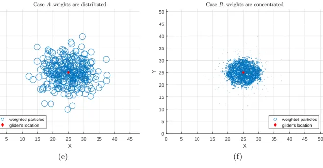
particles are discarded and high-weighted particles are replicated. In that process, when a small number of particles have higher weights, a large number of low-weighted particles are discarded. In this way, the probability mass accumulates on only those high-weighted particles which result in a smaller particle cloud. In contrast to that, when a large number of particles have similar weights, resampling cannot discard enough particles and the particle cloud becomes larger. Equation 2.7 shows that weight calculation of the particles directly relies on the variation of depth of those particles. To demonstrate the idea, let us consider the following case.
We want to compare the location estimation of the particle filter in two different locations A and B. Location A has very similar depth compared to its neighbours
(Figure 3.1a) which simulates A has flat surface. On the other hand, location B has significant uniqueness in depth compared to its neighbours (Figure 3.1b). Now, we have assigned random particle clouds on both of these locations and their neighbours. Both of the initial particle clouds are identical and randomly taken from a uniform distribution (Figure 3.1c and 3.1d). Next, we have taken the depth measurements and weighted the particles in both cases. The figures clearly shows that the lack of depth variation inA has distributed the weights among a large number of particles (Figure
3.1e) whereas the weights are concentrated in case of B (Figure 3.1f). The similar effect of depth variation is reflected in the resulting particle clouds. As expected, after resampling step, particle filter produced a larger cloud in A (Figure 3.1g) and
a significantly smaller cloud in B (Figure 3.1h). This suggests that the variation in
depth should help the particle filter as well as the glider TAN algorithm to achieve a better location estimation.
We want to quantify the contribution of depth variation such that this concept can be utilized in path planning. We are naming such quantificationratingand we are going to construct a function to calculate the rating without requiring to run particle
Surface elevation of the ocean with the location of the glider 95 100 40 50 Elevation 105 40 CaseA:flat surface Y 30 X 20 110 20 10 0 0 surface elevation glider's location (a) 95 100 40 50 Elevation 105 40
CaseB: variation in surface elevation
Y 30 X 20 110 20 10 0 0 surface elevation glider's location (b)
Initial particle cloud
0 5 10 15 20 25 30 35 40 45 50 X 0 5 10 15 20 25 30 35 40 45 50 Y
CaseA: particle cloud
particle cloud glider's location (c) 0 5 10 15 20 25 30 35 40 45 50 X 0 5 10 15 20 25 30 35 40 45 50 Y
CaseB: particle cloud
particle cloud glider's location
32
Weighted particles, larger circle indicates higher weight
0 5 10 15 20 25 30 35 40 45 50 X 0 5 10 15 20 25 30 35 40 45 50 Y
CaseA: weights are distributed
weighted particles glider's location (e) 0 5 10 15 20 25 30 35 40 45 50 X 0 5 10 15 20 25 30 35 40 45 50 Y
CaseB: weights are concentrated
weighted particles glider's location
(f)
Updated particle cloud which represents the location estimation
0 5 10 15 20 25 30 35 40 45 50 X 0 5 10 15 20 25 30 35 40 45 50 Y
CaseA: larger particle cloud
particle cloud glider's location (g) 0 5 10 15 20 25 30 35 40 45 50 X 0 5 10 15 20 25 30 35 40 45 50 Y
CaseB: smaller particle cloud
particle cloud glider's location
(h)
filter explicitly. To do so, first we need to decide what we should rate: a location or an area in the map.
3.1.1
Effectiveness of rating: a point vs an area
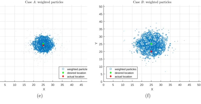
From the glider TAN algorithm, we have learned that only one depth measurement is taken in a given iteration and that depth is associated with the actual location of the glider in that particular iteration. By design, the rating must be pre-computable and the actual location of the glider will always be an unknown; therefore calculating the rating using the glider’s actual location is not a feasible option. Although we can compute the rating of an arbitrary location assuming the glider will be on that location, this approach does not give a good guarantee to reduce uncertainty. For instance, we can rate a location as good and expect the glider to visit and take a measurement at that location, but in reality, there is a good possibility that the glider may fail to reach that exact location and end up being on one of its neighbours. Taking a measurement at that neighbour may not be as useful as the desired location and the purpose of the rating function will be nullified in such cases.
To illustrate the above mentioned problem, we have run a particle filter twice on the same area for a different location of the glider. In both cases, the glider was expected to reach a location (denoted by the green diamond in Figure 3.2a) in the area. In the first case, we assumed the glider was able to reach that location and the resulting particle cloud has reduced adequately (Figure 3.2g). However, in the second case we assumed the glider was slightly displaced by ocean current and took a measurement at a neighbouring location (denoted by red diamond in Figure 3.2b). In this case, the particle filter did not estimate as good as before and the resulting particle cloud is larger (Figure 3.2h) than the one in previous case. We can also see that estimated location closely matches the glider’s actual location in the first case,
34
Surface elevation with the desired and the actual location of the glider
95 100 40 50 Elevation 105 40
CaseA: glider in desired location
Y 30 X 20 110 20 10 0 0 desired location actual location (a) 95 100 40 50 Elevation 105 40
CaseB: glider offthe desired location
Y 30 X 20 110 20 10 0 0 desired location actual location (b)
Initial particle cloud with desired and actual location
0 5 10 15 20 25 30 35 40 45 50 X 0 5 10 15 20 25 30 35 40 45 50 Y
CaseA: initial particle cloud
particle cloud desired location actual location (c) 0 5 10 15 20 25 30 35 40 45 50 X 0 5 10 15 20 25 30 35 40 45 50 Y
CaseB: initial particle cloud
particle cloud desired location actual location
Weighted particles, larger circle indicates higher weight 0 5 10 15 20 25 30 35 40 45 50 X 0 5 10 15 20 25 30 35 40 45 50 Y
CaseA: weighted particles
weighted particles desired location actual location (e) 0 5 10 15 20 25 30 35 40 45 50 X 0 5 10 15 20 25 30 35 40 45 50 Y
CaseB: weighted particles
weighted particles desired location actual location
(f)
Updated particle cloud with actual and estimated location
0 5 10 15 20 25 30 35 40 45 50 X 0 5 10 15 20 25 30 35 40 45 50 Y
CaseA: small estimation error
particle cloud desired location actual location estimated location (g) 0 5 10 15 20 25 30 35 40 45 50 X 0 5 10 15 20 25 30 35 40 45 50 Y
CaseB: higher estimation error
particle cloud desired location actual location estimated location
(h)
36
where as there is noticeable difference between them in the second one.
Considering the above example, we have reached the conclusion that computing the rating for a single location is not well suited for real world implementation. Rather, we have designed the rating function to rate a given area such that the rating value represents the overall quality of locations in that area. We are representing such area with a probability distribution and the following section describes more about that distribution.
3.2
Representing an area for rating
In the preceding section, we have shown that rating a single location is not appropriate for our real world application; a glider can attempt to reach a certain location and may end up at that location or any other nearby location. Assuming, the probability of the glider’s actual location is highest in the attempted location and the probability decreases as we move further away from that location, we can use bivariate normal distribution to represent the location probability of the glider. In our work, we are using X ∼ N(µ,Σ) to represent such distribution. X is a two dimensional random
variable containing the longitude and latitude and can be defined as X = [XY]T,
where X and Y are in global coordinate system and corresponds to the longitude
and latitude respectively. The variable µ denotes the mean of the distribution and
represents the location which the glider is attempting to reach. Σ is the covariance matrix of the distribution, (µ,Σ) corresponds to the area which the glider is expected to reach. We are assuming that the actual position of the glider will be anywhere within this area with higher probability of being at locationµand lower probabilities
3.3
Constructing the rating
The purpose of the rating is to take the glider’s location distributionX ∼ N(µ,Σ)1
as input along with a digital elevation model and to produce the expected location distribution X′ ∼ N(µ′,Σ′) after the glider takes an depth measurement. We are
naming the digital elevation model asmapdepth.
Now, from Σ and µ, we can determine the probability of the glider being on an
arbitrary location. Let us call these locationscellsand represent them usingi, where iranges over all relevant cells. In our work, a cell is an arbitrary location nearµsuch
that probability ofi is not negligible.
i = ix iy
The coordinate [ixiy]T of a celli determines the probability of glider reaching that
cell when aiming for µ. As X ∼ N(µ,Σ) is normally distributed, we can show that
the probability of celli depends on the distance between µand the celli. If we move
further away from µ the probability decreases. Similarly, the probability increases
if we move closer to µ and the highest probability is contained in the cell located
at µ. To calculate these probabilities, we need a probability density function. For
the bivariate normal distribution, the probability density function can be defined as follows P(i) = 1 2πq|Σ|e −1 2(i−µ) TΣ−1 (i−µ) (3.1)
whereP(i) is the probability of celli.
1It is important to haveµin the global coordinate system, but the rest of the calculation can be done using local coordinates. To avoid unnecessary calculation, we work in a local coordinate system that has the origin set toµ. This is not required for the rating process, but using local coordinates eliminates unnecessary computation.
38
We can look up the depth measurement zi of cell i using mapdepth. This implies
that if the glider is on cell i and takes a measurement, it should measure zi. Using
thezi, we can formulate the probability of measuring an arbitraryz at cell i. Ideally,
this probability P(z|i) should simply be defined as
P(z|i) = 1, if z =zi 0, otherwise
But in a real application, the above definition of P(z|i) is not appropriate. The
depth information inmapdepth may contain some error. In addition to that, the depth
measurement of the glider can be contaminated with instrument noise. We cannot correct the error contained inmapdepth, instead we can model this error and assign the
probability P(z|i) using that error model. We have used the error model (Equation
2.7) used in gTAN algorithm, defining P(z|i) as
P(z|i) = 1 σ2 DEM √ 2πe −(z−zi)2 /2σ2 DEM (3.2) whereσ2
DEM is the depth variance inmapdepth, and can be calculated using Equation
2.3. The instrument noise can also be modeled and integrated here, but the model will vary depending on the type and quality of instrument used to take the measurements. For simplicity, we are assuming instrument noise to be zero.
Now, P(i) in equation 3.1 provides the probability of being on a celli and P(z|i)
in equation 3.2 provides the probability of measuringz in that celli. Combining these
two probabilities, we can determine the overall probability of measuringz
P(z) = X
i
![Figure 1.1: Autonomous underwater vehicle: a Slocum glider [cF05]](https://thumb-us.123doks.com/thumbv2/123dok_us/1560952.2709438/13.918.260.715.107.453/figure-autonomous-underwater-vehicle-a-slocum-glider-cf.webp)