VARIANCE PREDICTION FOR POPULATION SIZE ESTIMATION
Ana I. Gómez
B,,Marcos Cruz and Luis M. Cruz-Orive
Department of Mathematics, Statistics and Computation, Faculty of Sciences, University of Cantabria, Avda. Los Castros 48, E-39005 Santander, Spain.
e-mail: [email protected], [email protected], [email protected] (Received July 28, 2018; revised March 5, 2019; accepted April 8, 2019)
ABSTRACT
Design unbiased estimation of population size by stereological methods is an efficient alternative to automatic computer vision methods, which are generally biased. Moreover, stereological methods offer the possibility of predicting the error variance from a single sample. Here we explore the statistical performance of two alternative variance estimators on a dataset of 26 labelled crowd pictures. The empirical mean square errors of the variance predictors are compared by means of Monte Carlo resampling.
Keywords: Cavalieri error variance predictor, geometric sampling, Monte Carlo resampling, particle counting, population size, Split error variance predictor, systematic quadrats.
INTRODUCTION
Population size is an important parameter for instance in ecology and social sciences. The target parameter is the size of a discrete population of objects, generally called ‘particles’. A particle is a compact set separated from other particles, serving as a model for a bird, a human, etc. In the present context the population is projected onto an observation plane which in practice is the plane of an image. The result is a finite setY ={y1,y2, . . .,yN} of N particle
projections contained in a bounded region of the plane, with the condition that all the particle projections are unambiguously distinguishable for counting. Thus, the effective particle population isY ⊂R2, and the target
is N – unobsevable original particles are ignored. In practice the sampling unit is a conveniently defined subset of a particle projection,e.g., a projected human head, or a distinguishable part of it, see Fig. 1a. For automatic resampling, however, each particle is replaced with an associated point, see Fig. 1b. Thus, henceforthyi∈Y may represent theith particle in the
‘real life’ sampling frame, or theith point particle in the ‘computer simulation’ sampling frame. For short, the former may be called the ‘real mode’, the latter the ‘computer mode’.
A design unbiased method to estimate N,
named CountEm (https://countem.unican.es/), based
on systematic quadrats, was recently proposed (Cruz et al., 2015; Cruz and González-Villa, 2018a;b). The method is familiar in quantitative microscopy, (Miles, 1978; Howard and Reed, 2005), and can be applied to any population that can be mapped onto an observation plane. In the real mode, a particle is sampled by a quadrat according to the forbidden line rule (Gundersen, 1977). In the computer mode,
however, a point particle is sampled if it is contained in the quadrat, simply.
The CountEm method is based on manual counting of reasonably small samples. By means of Monte Carlo resampling, Cruz and González-Villa (2018a) have shown that manually counting about 100 individuals, in about 30 nonempty systematic quadrats, usually yield coefficients of error (i.e., relative standard errors) below 10%, irrespective of population size. Apart from the bonus of design unbiasedness, with such small sample sizesCountEmis an attractive alternative to automatic methods, which are hitherto biased to unknown degrees (for references on the shortcomings of automatic particle detection see the latter paper and theIntroductionof Cruzet al., 2015).
An error variance predictor for the design unbiased estimatorNbofN, denoted by varCav(N), was presentedb
in Cruz et al. (2015). The estimator has a between
COUNTEM
METHOD
The idea of the method is to perform systematic sampling by superimposing on the population image a uniform random (UR) test grid Λx ⊂R2 of quadrats, see Fig. 1b, of a fixed orientation (namely a FUR test system, a term introduced by Miles and Davy, 1977). The adopted fundamental tile is a square J0=[0,T)2.
The tiles form a partition of the plane, and any tile
Jk of the test system can be brought to coincide
with J0 by a translation −τk that leaves the entire
test system unchanged. The fundamental probe is a squareT(0)=[0,t)2 ⊆ J
0, that is, 0<t≤T <∞. For
a description of test systems see Santaló (1976), or Gual Arnau and Cruz-Orive (1998). The probeT(0)is shifted intoT(x)=T(0)+xby a UR translationxwithin J0, dragging the entire test system into Λx =Λ0+x.
Thus,
Λx={T(x+τk), k ∈Z}, x∼UR(J0). (1)
Under the preceding design, an unbiased estimator (UE) of the population size N is the product of the sample size Q, namely the total number of particles counted with the grid under the aforementioned sampling rules, times the area sampling periodT2/t2,
that is,
b N=T
2
t2 ·Q. (2)
For a proof of the unbiasedness of Nb under the
computer mode (point particles, e.g., Fig. 1b) see Appendix S1 from Cruzet al.(2015). The unbiasedness property is independent from the orientation of the test system relative to the population. If the shape of the convex hull of the population image is nearly rectangular (as in Fig. 1b), however, then it is advisable to avoid parallelism between the edges of the image and the quadrat rows, or columns, in order to avoid an unduly large error variance. This idea is suggested in Fig. (11) from Gundersenet al.(1999). In the present experiment, each of the population images studied was framed by a rectangle, for which we adopted a common tilting angle of 30◦with respect to the base of the frame.
Cruz and González-Villa (2018a) propose a simple way to choose a grid compatible with preestablished values of the sample size and the number of nonempty quadrats.
Fig. 1. (a): Spectators in a football match (Bilbao, 1966), taken from Cancio (2010) with permission from the author. (b): Corresponding associated point particles, as used for Monte Carlo automatic resampling, with a tilted, FUR test grid of quadrats, superimposed on them. The fundamental tile is a square of sideT, the fundamental probe is a square quadrat of sidet∈ (0,T].
VARIANCE PREDICTORS
CAVALIERI VARIANCE PREDICTOR
even and odd rows, labeled e and o respectively in Fig. 1b). The result is equivalent to a grid of systematic quadrats with the latter parameters.
Next we define the necessary notation: •τ=t/T∈ (0,1], stripe sampling fraction.
•n: number of stripes encompassing the particle population,(n>2).
•ni: number of quadrats subsampled within the ith
stripe section,i=1,2, . . .,n.
•qi j: number of particles captured by thejth quadrat
within theith stripe, j=1,2, . . .,ni.
•Qoi,Qei: total numbers of particles captured by the odd numbered, and by the even numbered quadrats, respectively, within theith stripe.
•Qi=Ínj=i1qi j, total number of particles sampled in
theith stripe. Note thatQi=Qoi+Qei.
•Qo =ÍioddQi, Qe =ÍievenQi, total number of
particles on the odd numbered stripes and on the even numbered stripes, respectively.
•Q=Ín
i=1Qi, total number of sampled particles.
The Cavalieri variance predictor (Eq. 3 of Cruzet al., 2015) is:
varCav(N)b = c(τ)
τ4 [3(C0−bvn) −4C1+C2]+ bvn
τ4,
c(τ)= (1−τ)
2
6(2−τ),
Ck= n−k
Õ
j=1
QjQj+k, k=0,1,2,
bvn=
n
Õ
i=1
var(Qi).
(3)
The first term in the right hand side of the first Eq.3 estimates the between stripes variance contribution, whereasbvn/τ
4estimates the within stripes contribution,
which can be estimated by splitting the quadrat counts within the ith stripe into two subsamples with total countsQoi, Qei, respectively. Thus,
bvn=s(τ)
n
Õ
i=1
(Qoi−Qei)2,
s(τ)= (1−τ)
2
3−2τ .
(4)
SPLIT VARIANCE PREDICTOR
Here the between and the within stripes
contributions are both handled by means of the splitting
design adopted for v above. Thus, the corresponding predictor, alternative to Eq. 3, reads,
varsplit(N)b = s(τ)
τ4 [(Qo−Qe) 2−
bvn]+ bvn
τ4 . (5)
NEW MODIFICATION
In Cruz et al. (2015), the first Eq. 3, and Eq. 5, were computed for a single direction of the stripes (e.g., along the colums 0–7 in Fig. 1b). Here we have introduced the following, new modification: For each population, the mentioned predictors were computed first for a given direction of the stripes, and then for the perpendicular direction. In each case, the final variance predictor was the average of the corresponding two predictors.
In the figures, the predictors varCav(Nb) and varsplit(N)b are denoted byC1andS1, respectively, when computed along a single direction, and byC2andS2 when computed along two directions.
REMARKS ON NOTATION
In the sequel, true variances will be denoted by Var(·), whereas their predictors, or estimators, will be denoted by var(·). The true mean or expected value of a random variable (e.g., an estimator) will be denoted by E(·). For a positive random variable, the square coefficient of variation is CV2(·)= Var(·)/{E(·)}2. If the random variable is an estimator, then the equivalent notation CE2(·), called the square coefficient of error, is used.
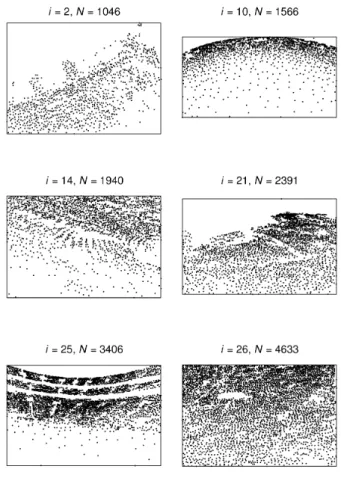
DATASET OF POINT PARTICLES
Fig. 2. Six of the 26 point particle populations constituting the dataset, ready for automatic Monte Carlo resampling. Each point was associated with a real particle from the original image, as in Fig. 1.
EMPIRICAL ASSESSMENT OF THE
VARIANCE PREDICTORS BY MONTE
CARLO RESAMPLING
The empirical variance ofNband the performances of varCav(Nb) and varsplit(N)b were evaluated by Monte Carlo resampling on each of the 26 point particle populations available with the aid of the R-spatstat package (Baddeleyet al., 2015).
For comparative purposes, the sampling fraction
was prescribed as f =Q/N, where Q=100, and N
was the known population size, namely the number of manually annotated points in each image. The initial numbers of quadrats considered were n0 =50
andn0=100. Practical prescriptions for the real case
in which N is unknown are provided by Cruz and
González-Villa (2018b).
As indicated in the preceding paper, with the prescribed pair{f,n0}, the grid parameters{t,T}were
computed as follows,
T = s
BxBy
n0
, (6)
t=Tpf ,
whereBx,By represent the width and the height of the
image frame, respectively. As mentioned in the second section, the resulting grid was tilted by 30◦with respect to the horizontal axis. Next we recall the necessary notation to describe the resampling procedure:
•Y = {y1,y2, . . .,yN} ⊂ R2: finite set – called the ‘population’ – of N point particles in a bounded area. Hereyi∈Y denotes theith point particle.
•Λx: FUR grid of quadrats, see Eq. 1 .
•Q: random number of point particles captured by the quadrats.
For each pair {t,T} a total of M≡K2 =322=1024 replicated superimpositions of the gridΛxontoYwere generated, corresponding toMsystematic replications of the point x within J0, arranged into a K×K UR
subgrid within J0 – this design should be expected to be more efficient than one of independent random replications (Cruz et al., 2015). We relabel the M systematic sites of the pointxas{xk, k=1,2, . . .,M}.
For each k, the corresponding sample total, Qk=Q(Y∩Λxk), (7)
was computed automatically. From Eq. 2, the kthUE
ofN is:
b
Nk=(T/t)2·Qk. (8)
For each population, the empirical mean, variance and square coefficient of error of Nb were computed respectively as follows,
Ee(N)b = 1 M
M
Õ
k=1
b
Nk, (9)
Vare(N)b = 1 M
M
Õ
k=1
h b
Nk−Ee(N)b i2
, (10)
CE2e(N)b =Vare(N)/Nb 2. (11)
On the other hand, to check the performance of the variance predictors we also computed the corresponding sets of M replicates {varCav(Nbk)} and
{varsplit(Nbk)}of the variance predictors, as well as the
corresponding square coefficients of error, namely, ce2(·)(Nbk)=var(·)(Nbk)/N2, (12)
interested in the behaviour of the numerator (i.e., in the variance predictor itself). The corresponding summary measure was computed as,
ce2(·)(N)b = 1 M
M
Õ
k=1
ce2(·)(Nbk). (13)
The preceding three equations are useful to illustrate the performance of the variance predictors graphically, see the next section. To describe the statistical performance of the variance predictors, however, we computed their mean square errors, namely,
MSEe(var(·)(N))b = 1 M
M
Õ
k=1
[var(·)(Nbk) −Vare(N)]b 2.
(14) Recall that, for an estimator ‘·’, MSE(·) =Var(·)+ Bias2(·). The first term in the right hand side of the preceding identity measures the variation of the estimator about its own mean, whereas the bias is the mean deviation of the estimator about the true value of the target parameter.
We will also use the normalized MSE, which we call the coefficient of MSE because it is analogous to the square coefficient of error, namely,
CMSEe(var(·)(N))b =
MSEe(var(·)(N))b Var2e(Nb)
. (15)
As advanced in theIntroduction, for a given set of sampling parameters we want to compare the statistical performance of the Cavalieri and the Split variance predictors on each ofn=26point particle populations of sizesN1,N2, ...,Nn. For theith population we define
the relative empirical accuracy of the latter to the former predictor as follows (e.g., Lindgren, 2017),
RAi(Cav,Split)=
MSEe(varsplit(Nbi)) MSEe(varCav(Nbi))
. (16)
For instance, if RAi(Cav,Split)>1, then the Cavalieri variance predictor is ‘better’,i.e., more accurate, than
the Split one for the ith population, in the sense
that it has the smaller MSE there. If the variance predictors involved were unbiased, then the RA index would be the usual relative efficiency ratio. As a global numerical summary from thenpopulations we propose the relative empirical accuracy index as
RA(Cav,Split)= Ín
i=1MSEe(varsplit(Nbi)) Ín
i=1MSEe(varCav(Nbi))
. (17)
RESULTS
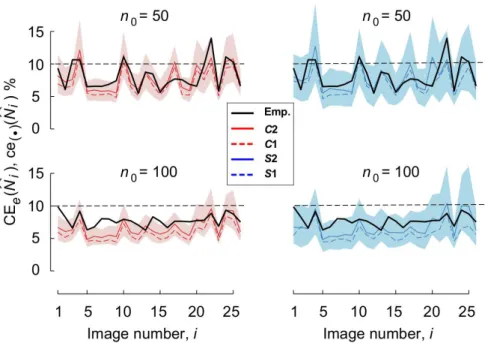
For each of the 26 populations, for each variance predictor, and for each of two different sampling intensities, the descriptors CE2e(Nbi) and ce2(·)(Nbi)
defined above are represented in Fig. 3 by a black and a coloured line, respectively. When computed using a single direction, the latter values are linked by a coloured broken line. Here Nbi denotes the UE of Ni, (i=1,2, ...,n=26). In addition, for each predictorC2
and S2 the M = 1024 individual replications given
by the square root of Eq. 12 are enclosed within the corresponding 95% confidence bands.
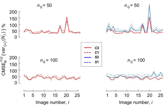
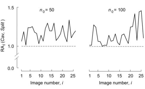
For each of the mentioned cases, Fig. 4 displays the corresponding CMSE1/2’s, namely the square roots of Eq. 15. Further, Fig. 5 displays the individual relative accuracy indices computed via Eq. 16. Finally, the summary RA indices computed with Eq. 17 are displayed in Table 1.
Table 1. Summary indices of relative accuracy (RA)
computed via Eq. 17. The abbreviationsC1, S1,C2, andS2are defined in the subsection ‘New modification’.
n0=50 n0=100
RA(C2,S2) 1.17 1.13 RA(C1,S1) 1.21 1.16 RA(C2,C1) 1.01 1.08 RA(S2,S1) 1.05 1.11
DISCUSSION AND CONCLUSIONS
A new error variance predictor, called the Split predictor, varsplit(Nb), was proposed for the CountEm population size estimator. Its performance was tested against the current Cavalieri predictor, varCav(N), on ab dataset of 26 point particle populations.
The Cavalieri variance predictor was statistically better than the Split predictor for the dataset considered, in the sense that the individual relative accuracy ratios, see Eq. 16, were always greater than 1, see Fig. 5. In this graph the variance predictors wereC2, S2, as defined in the subsectionNew modification. The corresponding summary index RA(C2,S2) also reveals a superiority ofC2overS2, see Table 1. However, the mean values of ce(·)(Nbi)for the individual populations, represented by red and blue continuous lines in Fig. 3, were rather similar amongC2andS2for each value ofn0. This is
Fig. 3.Behaviour of the empirical, and the mean predicted, coefficients of error of the number estimators, computed for each particle population as the square roots of Eq. 11 and Eq. 13 respectively. The coloured bands enclose the95%of the Monte Carlo replications computed for each population as the square root of Eq. 12. The inset symbols are defined in the subsection ’New modification’.
Cavalieri disectors under the Cavalieri and the Split designs, see Fig. 8 of the latter paper.
With the new modification the variance predictors were globally at least as accurate as the ones computed in a single direction, as shown in Table 1. For individual populations, however, there were some exceptions, see Fig. 4. Table 1 also suggests that the gain in precision due to this modification was more important forn0=100than forn0=50.
Both variance predictors often underestimated the empirical empirical error variance, see Fig. 3. As shown in Fig. 4, however, the relative MSEe(var(·)(Nbi)), see Eq. 15, tended to be larger forn0=100than forn0=50.
We conjecture that this may be due to the fact that with
n0 =100 the mean number of particles per quadrat
decreases, this tending to induce independence among quadrat counts. Recall that either variance predictor relies on modelling quadrat count dependence using G. Matheron’s transitive theory – hence the predictors tend to be less accurate under quadrat count independence.
In short, based on the RAiand RA relative accuracy
indices, for the dataset studied the preferred predictor was C2, namely varCav(N)b computed as the average among the two contributions along the two mutually perpendicular stripe directions of the quadrat grid.
ACKNOWLEDGEMENTS
The authors acknowledge financial support from the AYA-2015-66357-R (MINECO/FEDER) project.
REFERENCES
Baddeley A, Rubak E, Turner R (2015). Spatial Point Patterns: Methodology and Applications with R. New York: Chapman and Hall/CRC.
Cancio R (2010). Simplemente ... Periodismo. Madrid: Ediciones APM.
Cruz M, Gómez D, Cruz-Orive LM (2015). Efficient and unbiased estimation of population size. PLoS ONE 10:e0141868.
Cruz M, González-Villa J (2018a). Simplified procedure for efficient and unbiased population size estimation. PloS ONE 13:e0206091.
Cruz M, González-Villa J (2018b). Unbiased population size estimation on still gigapixel images. Sociol Method Res 0049124118799373.
Cruz-Orive LM (2004). Precision of the fractionator from Cavalieri designs. J Microsc 213:205–11.
Cruz-Orive LM (2006). A general variance predictor for Cavalieri slices. J Microsc 222:158–65.
Fig. 4.Behaviour of the coefficient of square root mean square error, computed for each particle population as the square root of Eq. 15, in percent. The inset symbols are as in Fig. 3.
Gual Arnau X, Cruz-Orive LM (1998). Variance prediction under systematic sampling with geometric probes. Adv Appl Probab 30:889–903.
Gundersen HJG (1977). Notes on the estimation of the numerical density of arbitrary profiles: the edge effect. J Microsc 111:219–23.
Gundersen HJG, Jensen EBV, Kiêu K, Nielsen J (1999). The efficiency of systematic sampling in stereology — reconsidered. J Microsc 193:199–211.
Howard CV, Reed MG (2005). Unbiased Stereology. Three-dimensional Measurement in Microscopy, 2nd Ed. Oxford: Bios/Taylor & Francis.
Idrees H, Saleemi I, Seibert C, Shah M (2013). Multi-source multi-scale counting in extremely dense crowd images. In: Proc IEEE Conf Comput Vision Pattern Recogn (CVPR) 2547–54.
Lindgren B (2017). Statistical Theory. Routledge.
Matheron G (1971). The Theory of Regionalized Variables and its Applications, vol. 5. Les Cahiers du Centre de Morphologie Mathèmatique de Fontainebleau, No. 5. Fontainebleau: École national supérieure des mines de Paris.
Miles RE (1978). The sampling, by quadrats, of planar aggregates. J Microsc 113:257–67.
Miles RE, Davy P (1977). On the choice of quadrats in stereology. J Microsc 110:27–44.
Santaló LA (1976). Integral Geometry and Geometric Probability. Addison-Wesley, Reading, Massachusetts.
APPENDIX: HINTS ON THE
DERIVATION OF THE ERROR
VARIANCE PREDICTORS
LetY ⊂R2represent a finite population ofN point particles contained in a bounded region of the plane. Fix a sampling axisO x, and let L(x)denote a straight line normal to O x at a point of abscissa x. A stripe Lt(x) of thickness t > 0 is the portion of the plane
comprised between the two parallel lines L(x) and
L(x+t). LetQt(x)denote the total number of particles
captured byLt(x), namely the cardinality ofY∩Lt(x).
For Matheron’s transitive theory to work, it is necessary to assume that there exists a function f : R→R+such that,
Qt(x)=
∫ x+t
x
f(y)dy, x∈R, (18)
in which case,
N= 1 t
∫
R
Qt(x)dx, (19)
see Cruz-Orive (2006), who gives a chronological account on the evolution of the problem.
Consider a FUR test systemΛ1of Cavalieri stripes of thicknesst and periodT, 0<t≤T <∞, normal to the sampling axis. Let {N1,N2, ...,Nn}, n≥3, denote
Fig. 5.Relative accuracy ratio for each particle population, computed via Eq. 17. The variance predictors involved wereC2andS2.
numbers, respectively. For each i =1,2, ...,n, let Nbi
denote an UE ofNi. An UE ofNis,
b N=T
t
n
Õ
i=1
b
Ni. (20)
A predictor of Var(N)b is,
var(N)b = c(τ)
τ2
h
3(Cb0−bνn) −4Cb1+Cb2 i
+bνn
τ2,
τ=t/T,
c(τ)= (1−τ)
2
6(2−τ),
b Ck=
n−k
Õ
j=1
b
NjNbj+k, k=0,1,2,
bνn=
n
Õ
i=1
var(Nbi),
(21)
which is Eq. 3.3 from Cruz-Orive (2006) with the smoothness constantq=0, because the function f is expected to have finite jumps – thus,c(τ) ≡α(0, τ), see the first Eq. 3.7 of the same paper. The predictor is based on a fractional model of the covariogram of f near the origin, see Eq. II.1 of that paper. The last Eq. 21 assumes that the within stripe deviations{Nbi−Ni}are mutually uncorrelated. Note that the symbolbνnin 21 is different frombvnin Eqs. 3 and 5.
Consider now an independent FUR test systemΛ2
of Cavalieri stripes with the same parameters {t,T},
perpendicular toΛ1. Clearly Λ1∩Λ2 is the FUR test system of quadratsΛxdefined by Eq. 1. It is now easy to see that
b
Ni=τ−1Qi, (22)
is an UE of Ni, where Qi is as defined for Eq. 3.
Therefore,
b
Ck=τ−2Ck, (23)
whereCk is given by the third Eq. 3. Moreover,
var(Nbi)=τ
−2var(Q
i). (24)
Substitution of the preceding two results into the right hand side of the first Eq. 21, the predictor given by the first Eq. 3 is obtained.
An alternative approach to treat FUR Cavalieri stripes is the Split design. The first stage sample {N1,N2, ...,Nn} generated by Λ1 is split into two
systematic subsamples consisting of the odd and even numbered particle counts, respectively. Let No, Ne denote the corresponding total point particle counts, and Nbo, Nbe the respective unbiased estimators. The development follows Matheron’s theory, as above, with
smoothness constant q = 0, and the corresponding
variance predictor is given by Eq. 2.27 from
Cruz-Orive (2004), which was derived for a numbern ≥2
var(N)b = s(τ)
τ2
h
(Nbo−Nbe)2−bν2) i
+bν2
τ2,
τ=t/T,
s(τ)=(1−τ)
2
3−2τ ,
bν2=var(Nbo)+var(Nbe).
(25)
When the perpendicular FUR stripes fromΛ2intersect
Λ1we have,
b
No=τ−1Qo, Nbe=τ−1Qe, (26)
whereby,
b
ν2=τ−2
n
Õ
i=1
var(Qbi)=τ −2
bvn. (27)
Substitution of the preceding two results into the right hand side of the first Eq. 25, yields Eq. 5.
The Split design is now used to predict each within stripe variance by means of the first Eq. 25 withbν2=0, because the quadrat counts Qoi and Qei are directly
observable. Thus,
var(Qbi)=s(τ)(Qoi−Qei)2, (28)
which, combined with Eq. 27, yields Eq. 4.
The same results apply when point particles are replaced with arbitrary particles, the stripes with stripe disectors, and the quadrats with unbiased frames, (this is the ‘real mode’ mentioned in the Introduction). For illustrations of both the Cavalieri and the Split designs see also Cruz-Orive and Geiser (2004). The combinations given by Eq. 3 and Eq. 5 for quadrats, however, were first proposed by Cruz et al. (2015), (without proof). The idea was to treat the between stripe contribution with the Cavalieri model, and the within stripe contribution with the Split model. The individual quadrat counts {qi j} will tend to be small (usually between 0 and 5) – hence it is sensible to add them up into two groups (consisting of the odd and
even numbered quadrat counts), which is what the Split method does for the within stripe variance contribution.
Generalization. The generalization of Eq. 21 to higher dimensions is relatively straightforward. Consider for instance a series of FUR Cavalieri slabs in R3, and hit this series with a perpendicular FUR series. The result is a three dimensional grid of FUR bars whose cross section is a square of side length t. In Fig. 1b, the bars would be perpendicular to the plane of the paper, and they would be viewed as quadrats. The particle contents Ni of the ith slab
would be unbiasedly estimated from the contents of the Cavalieri bars subsampled within it. Thus, up to this second stage the error variance would be predicted by the first Eq. 21, and bνn would be predicted by the last Eq. 21. Now, however, Nbi would be an UE of Ni
computed as T/t times the total contents of all the Cavalieri bars subsampling theith slab. Consequently, var(Nbi) could be predicted again by the first Eq. 21 with a proper readaptation of the symbols. Thus, the two stage predictor of var(N)b would be a nested version of two Cavalieri components, one accounting for the variation among slabs, and the other for the variation among bars within slabs. The third stage probe would be a FUR Cavalieri series of slabs perpendicular to the other two: in Fig. 1b, this last series would be parallel to the plane of the paper. The intersection between the three mutually orthogonal slab series would be a three dimensional cubic grid of cubic blocks of side length t, and the sampling volume period of the grid would be (T/t)3. The final variance predictor ofNbwould be the aforementioned nested predictor with the two Cavalieri components, plus a third nested component accounting for the variation of blocks within bars, which could now be computed using the Split predictor formula. Thus, within each bar the third component would be analogous to Eq. 28 withQoi,Qeirepresenting the total