Vol 12, No 2 (2020)

Image Malware Detection using Deep Learning

Jamal El Abdelkhalki, Mohamed Ben Ahmed, Boudhir Anouar Abdelhakim

Computer Science, Systems and Telecommunication Laboratory, (LSIT), University AbdelmalekEssaadi, Tangier, Morocco

Abstract: We are currently living in an area where artificial intelligence is making out every day to day life much easier to manage. Some researchers are continuously developing the codes of artificial intelligence to utilize the benefits of the human being. And there is the process called data mining, which is used in many domains, including finance, engineering, biomedicine, and cyber security. The utilization of data mining, artificial intelligence algorithms like deep learning is so vast that we can't even name them all. This technology has almost touched every industry and cyber security is the most beneficial. The process of enhancing cyber security with the help of deep learning methods has come out of the theory books and many organizations are utilizing them rather than using a traditional piece of software to defend against online threats. Especially in the field of recognizing and classifying codes or malware. And this is essential, because, with the advent of cloud computing and the Internet of Things, expand potential malware infection sites from PCs to any electronic device. This makes our day to day life very unsafe. In this post, first, we will describe in brief how deep learning can be the most useful and promising techniques to detect malware. Besides this we will go through a deep neural network, ResNet for malware dynamic behavior classification jobs.

Keywords:Malware,detection,Malware,CNN,ResNet, Cyber security.

1.

Introduction

Nowadays, data analysis is a crucial step for any project in several areas such as IT, marketing, finance. In this context, the analysis of the log files motivated a large number of researchers. The latter conducted their research studies on the different data are in the volumetric log files[1].This particular method of data analyzing is showing a promising feature in the context of malware detection. Therefore, Malware detection is a process of analyzing any suspicious applications that exist in the PC[2]. It is a key part of software safety research.

Generally, to detect and classify malware, there are clear sets of detection methods. Since there are many methods to detect malware, the result is not the same all the time. Most of the time, we see users are making use of generic anti-virus software to shield against malicious applications or software. However, this is not a trustworthy system, to begin with[3].This software most of the time are unable to classify and unable to detect malware mutation, variants, and rapid code changes. As a result, the user left the PC vulnerable to numerous threats.What is making his worse is the continuous changes in the way malicious software or codes are being made. And, besides this, every now and then there's new malware popping up in the market. According to "China Internet Security Report for the First Half of 2018": with the help of 360 Internet Security center, researchers found out that in the

first half of 2018 alone, there were more than 140 million occurrences of new malicious programs, which were detected by the Internet Security software and 795,000 new malicious software were being intercepted regularly. Amongst them, the number of malicious software built for

the PC was 149,098,000 hence 779,000 new harmful applications were being intercepted per day. The same program detected about 2.831 million malicious programs build to affect the Android platform, and they were intercepting about 16,000 new malicious programs every day. After going through the stats, we can obviously see why it is becoming more and more difficult to find a suitable solution to detect malware. However, it is a concern for everyone who needs a proper and efficient answer[4]. The method that can actively used in order to answer to the problem of detecting or classifying malware, is the method of deep learning.

In this paper, we study, at the beginning, the research work in relation to malware especially those based in detection malware using different methods. We presented a deep learning model for malware detection using malware image. Deep learning is widely used in image recognition.

2.

Related works

Family since different anti-virus software has different tags for one group. Marcos Sebastiain[5] advocated AV Class which makes use of the semantic analysis of malicious program name tags produced by various engines to recognize the same familiarly Bartos[6] stated that undiscovered malicious code variants could be identified by drawing out statistical characteristics from the network stream without proper code fingerprints features. YuFeng et al. [7] advised to make use of a method called ASTROID. This exceptional method can automatically extract common malicious features from a known malware family database to detect new malicious codes. This technique changes the homogeneous harmful code detection into highest satisfiability problem solving by exploring the most suspicious common subgraph (MSCS) from a small number of identified malware family examples. The outcomes show that the suggested method is better to the manual technique in detection efficiency and accuracy rate, also can defeat behavioral obfuscation and other counter measures. Advancement of malware technologies. And today, if we research a bit about different types of malware detection technologies, we will be able to find a few exceptional detection methods of malware codes, and here they follow: Rules-based method[8], Heuristic Analysis[9], DNA Analysis[10],and Deep Learning Method[11], [12].

classes and some make images of machine language code to classify given malware, while other use hybrid approaches. To summarize, malware image analysis highlighted in the related works. However ,a huge effort still required to progress and promote the system efficiency. In this purpose, it is necessary to monitor and detect malware by following specific methodologies using deep learning and provide a prediction of malware image.

3.

Background

3.1 Deep learning

Deep learning or deep neural networks (DNNs) takes inspiration from how the brain works and forms a sub module of artificial intelligence. The main strength of deep learning architectures is the capability to understand the meaning of data when it is in large amounts and to automatically tune the derived meaning with new data with brand-new data without the necessity for an area expert knowledge. Convolutional neural networks (CNNs) and Recurrent neural networks (RNNs) are two types of deep learning architectures predominantly applied in real-life scenarios. Generally, CNN architectures are used for spatial data.

The concepts behind the various deep learning architectures are discussed in a mathematical way.

3.1.1 Deep Neural Network (DNN)

DEEP NEURAL NETWORK (DNN) A feed forward neural network (FFN) creates a directed graph in which a graph is composed of nodes and edges. FFN passes information along edges from one node to another without formation of a cycle. Multi-layer perceptron (MLP) is a type of FFN that contains 3 or more layers, specifically one input layer, one or more hidden layer and an output layer in which each layer has many neurons, called as units in mathematical notation. The number of hidden layers is selected by following a hyper parameter tuning approach[14].

A (FFN) feed forward neural network creates a directed graph in which a graph is composed of nodes and edges. The information passed by the FFN along edges from one node to another without formation of a cycle. (MLP) Multi-layer perceptron is a type of FFN that contains 3 or more layers, precisely one input layer, one or more hidden layer and an output layer in which each layer has many neurons, called as units in mathematical notation. The number of hidden layers is selected by following a hyper parameter tuning approach. The transformation of information from one layer to another is done in the direct without considering the past values. Moreover, neurons in each layer are fully connected .An MLP with n hidden layers can be mathematically formulated as given below:

𝐻(𝑥) = 𝐻𝑛(𝐻𝑛−1(𝐻𝑛−2(• • • (𝐻1(𝑥))))) (1) H defines hidden layer. This way of stacking hidden layers is typically called as deep neural networks (DNNs)[Fig 1]. shows a pictorial representation of DNN architecture with n hidden layers. It takes input:

𝑋 = 𝑋1, 𝑋2, • • •, 𝑋𝑝−1, 𝑋𝑝(2)

𝑎𝑛𝑑𝑜𝑢𝑡𝑝𝑢𝑡𝑠: 𝑂 = 𝑂1, 𝑂2, • • •, 𝑂𝑐−1, 𝑂𝑐 (3)

Each hidden layer uses Rectified linear units (ReLU) as the non-linear activation function. This helps to reduce the state of vanishing and error.

Figure 1. Architecture of DNN with n hidden layers Gradient issue. ReLU has been turned out to be more proficient and capable of accelerating the entire training process altogether[15]. ReLU is defined mathematically as follows:

𝑓 (𝑥) = 𝑚𝑎𝑥(0, 𝑥) (4) Where x denotes input

3.1.2 Convolutional Neural Network (CNN)

Before we review how deep learning is employed for malware classification, let us revisit how convolutional neural networks are used for image classification. An image is input to the network in its raw pixel format. The image goes through a sequence of convolutional layers which can be viewed as automatically computing image features at different levels of abstraction. The spatial dimension of feature maps decreases due to max pooling layers. Neurons in higher layers correspond to larger receptive fields of pixels in the input image over which features are being computed. These convolutional layers are followed by fully connected layers (dense layers), or in more modern architectures, by global average pooling layer. Right in the end, we have classification output layer which outputs probabilities of the image being in different categories. For speech recognition, we can convert speech signal into a 2-D image called spectrogram in which time is one axis and other is frequency, and we can apply similar techniques[16].

sequence related information. Finally, the LSTM features are passed into fully connected layer for classification [17]. Convolutional layers: These layers apply a certain number of convolution operations (linear filtering) to the image in sequence. Typically, these filters extract edge, color, and shape information from the input image. Basically, the filters operate on subregions of an image and perform computation such that it produces a single value as output for each subregion. The output (say x) of this layer is typically forwarded to a non-linear function (called ReLU activation) which is defined as:

(𝑥) = (0, 𝑥) (5)

Pooling layers: This layer is responsible for down sampling (i.e. reducing the spatial resolution of the input layers) the data produced from convolution layers so that processing time can be reduced, and so that computational resources can handle the scale of the data. This is due to that fact that as a result of pooling, the number of learnable parameters is reduced in the subsequent layers of the network. Max pooling is a commonly used pooling technique that keeps the maximum value in a region (e.g. 2x2 non-overlapping regions of data) and discards the remaining values.

Fully connected layers: This layer performs classification on the output generated from convolution layers and pooling layers. Every neuron in this layer is connected to every neuron present in the previous layer. This type of layer is typically followed by a Dropout layer that improves the generalization capability of the model by preventing over-fitting which is commonly occurring problem in deep learning domain [18] [Fig 2].

Figure 2. Architecture of CNN for malware detection[14]

3.2 Transfer learning

Transfer learning is what we do every day, it is to take advantage of learning acquired previously, to, by analogy, solve a similar but different problem. The transfer learning of neural networks is based on the same principle. If we trained a neural network to differentiate malware, benign, from photos, then we can rely on this network to guess what category malware belongs to. And even better. This is possible because neural networks are stacked in layers, each learning from the previous. This is how a CNN (neural network by convolution) will have its first layers specialized in the recognition of simple shapes (horizontal lines, vertical lines, diagonals, ...), its following layers dedicated to the recognition of shapes a little more complex (circle, square, triangle,…), its following layers oriented towards, for example recognition of faces, recognition of body parts,…. and the final layers will focus on what is being learned from this network (malware or benign). During the learning phase, the neural network changes its weights. The weights (which are numbers) and the architecture of the network are

sufficient to characterize it (apart from a few parameters not described here). It is therefore very easy to benefit from an existing neural network, without having to recalculate what has enabled it to reach its optimal configuration, calculated for the dataset and the problem for which it was designed [Fig 3] [19].

Figure 3. Transfer learning

3.3.Residential Energy Services Network (ResNet)

Unfortunately, deep CNNs are hard to train due to vanishing gradients in the long forward feed and backward propagate process. A residual neural network, on the other hand, has shortcut connections parallel to the normal convolutional layers. Mathematically, A ResNet layer approximately calculates:

𝑦 = 𝑓(𝑥) + 𝑖𝑑(𝑥) = 𝑓(𝑥) + 𝑥 (6)

Those shortcuts act like highways and the gradients can easily flow back, resulting in faster training and much more layers. The winner model that Microsoft used in ImageNet 2015 has 152 layers, nearly 8 times deeper than best CNN [Fig 4][20].

Figure 4. A deeper residual function F for ImageNet[21] In order to detect malware and compute the accuracy, we applied CNN. The CNN can be based on several different models like VGG nets, GoogleNet model, ResNet model… In this study, we utilized the ResNet model because it has tremendous performance as compare to the other models[22]. In this article, we will not consecrate it to give more details about the comparison between the others models and ResNet model but we will go with another comparison more important compared to our study, it is the comparison between the architectures of ResNet (18, 34, 50, 101, 152). For further, there is several of ResNet model’s architectures, it depends on number of hidden layers.

As we said before, Resnet is one of the most powerful deep neural networks- until now- which has achieved excellent performance results concerning the classification of Malware. We can find many different ResNet architecture (The same concept but with a different number of layers: 18, 34, 50, 101, ResNet-110, ResNet-152).

the other architectures of ResNet (50, 101,152) used three layers deep [Fig 5].

In order to get 50- layer ResNet, the block with three layers replace the block with two layers in the 34-layer net. This model has 3.8 billion FLOPs. The same method is applied with 101-layer and 152-layer ResNets, they are constructed by using more 3-layer blocks Even after the depth is increased, the 152-layer ResNet (11.3 billion FLOPs) [Fig 5].

Figure 5. Sizes of outputs and convolutional kernels for ResNet[28]

4.

Methodology of the proposed models

4.1Malware detection

The machine learning approach to predict the capability of countering a code mutation, variation and reverse engineering of the codes, which can be used to determine the strength of the harmful alien code obfuscation variants that produced soon afterward[23]. This method is effective against successfully predict or counter the new malicious samples and recognize the class variants by making use of deep learning method. And there's a possibility to use this technique to automate the detection of malware which will reduce a lot of human resources and efforts. It is a promising chapter of malware detection technology and can offer a new path for anti-malware research and application.

4.2 The proposed system

In this section, we introduce a deep learning model for malware detection using malware image. Deep learning is widely used in image recognition. Especially convolutional neural network CNN is mainly used. In neural network, each node in the previous layer gives effects to all node in the next layer. However, in CNN, only several nodes in the current layer give effects to the nodes in the next layer.so, CNNs are able to use local correlation. It means that CNN learns features from the image.

Using the process of training and inference framework has a similar process, during the training phase, a known set of data is transmitted to an untrained neural network. The results of the framework are compared to the results of known data sets. Next, the framework reassesses the error value and updates the weight of the data set in the layers of the neural network depending on how the value is correct or incorrect. This reassessment is very important for the training stage because it adjusts the neural network to improve the performance of the next task that it learns. In contrast to training, inference does not reassess or adjust the layers of the neural network based on the results. Inference infers the

knowledge of a trained neural network model and uses it to infer a result. Thus, when a new unknown data set is entered via a trained neural network, it generates a prediction based on the predictive accuracy of the neural network. Inference comes after training because it requires a trained neural network model. While a deep learning system can be used for inference, the important aspects of inference make a deep learning system not ideal. Deep learning systems are optimized to handle large amounts of data to process and re-evaluate the neural network. This requires high performance computing which is more energy, which means more costs. The inference can be smaller data sets, but hyper-calibrated to many devices [Fig 6].

Figure 6. Model of detection malware

5.

Data Preparation and Environment Setup

In this segment, we present details regarding dataset numbers for both malware & benign apps. Additionally, this segment represents how we set up the test conditions to observe behavior for these applications.

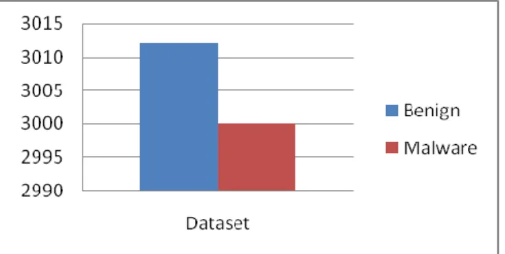
To evaluate the effectiveness of classical machine learning and deep learning architectures, it is required to create a large data set with a variety of different samples. The publicly available data sets for possible research in cyber security for malware detection are very limited due to the privacy preserving policies of the individuals and organizations. Over time, as malware have grown it has become increasingly difficult to have one source having all types of malware families. Many researchers try to collaborate their findings but still there is not a single dataset or repository to acquire all the required samples. In this research, the publicly available dataset contains 3000 benign and 3012 malware which were split up into the following: training dataset (60%), validation data (20%), and testing data (20%). The training dataset was shuffled but the validation and testing dataset were not.[Fig 7].

Figure 7. Data set of malware detection

Multi-class Multi-classification can also be done using this technique, with the idea being that a variant of malware files will have images different from the other.

[Fig 8] presents all steps of the architecture of our system. First of all, we started with download malware and begin software from open source databases (Download), after that we extract this files that contain malware and benign software (Unpacking). The third step is the operation code from each instruction and then produces a data set in which each instance is described by sequences of opcodes(Opcode). Next, the binary image matrices are reconstructed by these opcode sequences with their probabilities and information gains (Binary image). Later, we split dataset into two parts training and testing phases (Split Dataset). The next step is to implement fastai in PytTorch of the models ResNet:18, 34, 50, 101 and 152 (Implement the models). After that, we optimize the model to reduce Learning Rate (Reduce LR). The last step is prediction on test dataset (Malware or Benign).

Figure8. Architecture for proposed model from data preparation to prediction

Once we have our dataset ready, we will convert each file into a 256x256 grayscale image (each pixel has a value between 0 and 255)[Fig 9].

Since malware detection is done in real time, we need to classify an image as benign or malware within seconds. Therefore, keeping the image generation process simple and short will help us save valuable time.

We used fastai for PyTorch library to implement the image classification with Google Colaboratory tool for the purpose of classification, the below shows the Neural Network generated by the Deep Learning technique.

Fastai is a deep learning library that provides researchers with high-level components that can quickly and easily achieve good cutting-edge results in standard deep learning areas and provides researchers with low-level components that can be mixed and matched to create new patterns. It aims to do both things without substantial compromise in ease of use, flexibility or performance. This is possible through a carefully layered architecture, which expresses the common underlying models of many deep learning and data processing techniques in terms of decoupled abstractions. These abstractions can be expressed concisely and clearly by taking advantage of the dynamism of the underlying python language and the flexibility of the PyTorch library.

Fastai includes: A new type distribution system for Python with a semantic type hierarchy for tensors A computer vision library optimized by GPU which can be extended in pure Python An optimizer which refactors the common functionalities of modern optimizers into two elements basic, allowing the algorithms to optimize the code. A new bidirectional callback system that can access any part of the data, the model or the optimizer and modify it at any time during training A new API from data block and much more. In this article we have used this library to create our own comprehensive deep learning model for detecting malware on different images. The library is already widely used in research, industry and education [24].

Figure 9. Benign image (left) and malware image (right)

6.

Experiments and Evaluation

In this paper, we are going to cover ResNet-152 in detail which is the most efficient one for our system. More details and explanation are presented in this axis.

In order to compare the models of ResNet, our system calculates four parameters (Accuracy, Precision, Recall and F1 score) using four main evaluation metrics [Table 1]:

Table 1. Evaluation metrics of each indicator

Indicator Formula

Accuracy

Precision

Recall

F1 Score

Here below the explanation of each indicator: Accuracy is a measure of correct classification.

Precision is a measure of accurate positive predictions over the total amount of positive predictions.

Recall is a measure of true positive over total actual positive. F1 score is used whenever there needs to be a balance between Precision and Recall and there is a large imbalance in the dataset[Table 1] [25].

As we can see in the figure above, our system used four main parameters to calculate the accuracy, the precision, the recall and the F1 score.

Figure 10. Confusion matrix

Each parameter of confusion matrix is explained below: TP: True Positives is the number of correctly identified malware samples.

TN: True Negatives is the number of correctly identified benign samples.

FP: False Positives is the number of samples that were benign but identified as malware.

FN: False Negatives are the samples that were malware but not identified correctly by the model[25].

[Table2] shows the results of each ResNet model (18, 34, 50, 101 and 152) considered in this research.

Accuracy: The base models ResNet 18 and ResNet 34 reached the lowest value accuracy with a negligible difference in which ResNet 18 presents 87,9% and ResNet 34 presents 87%. Note that ResNet 101 with an accuracy of 91% and ResNet 50 with an accuracy slightly better of 91,6% perform so good but they still not the best compared to ResNet 152 with the highest accuracy of 93,5%.

Precision: The ResNet 34 have noticeable lower precision than all the other model with a percentage of 87,3% followed by ResNet 18 with a precision of 88,5%, that means that they are incorrectly classifying benign samples as malware. ResNet 101 and ResNet 50 achieved a high precision of91,8% and 93,2% successively but they still lower than the precision achieved by ResNet 152 (93,4%). That indicates that most samples classified as infected was indeed infected for this model (ResNet 152).

Recall: All ResNet models were close but ResNet-152 was the best (95%). Since recall is a measure of many infected samples where missed by the models, ResNet 152 seem to be effective at identifying most infected samples. A high recall score suggests that the model is strong at identifying less obvious malware samples.

F1 Score:ResNet 152 model scored the highest with a score of 94,1%. That indicates ResNet 152 has the best balance of precision and recall. In other word, it has the best balance between identifying only malware samples and identifying most of infected samples over all[Table 2].

Concerning the detection time, we have reserved a part just above.

Table 2. Results of confusion matrix for each ResNet model

Model Accuracy Precision Recall F1

score Time (s)

ResNet 18 0,879 0,885 0,90 0,892 37

ResNet 34 0,87 0,873 0,91 0,891 40

ResNet 50 0,916 0,932 0,916 0,923 43

ResNet 101 0,91 0,918 0,933 0,925 51

ResNet 152 0,935 0,934 0,95 0,941 56

We present the table above as a graph in order to simplify the overview. We can see clearly why we choose ResNet 152 in our system (Best accuracy 93,5%, best precision 93,4%, best recall 95% and best F1 score 94,1%)[Fig 11]. So, we can say it is the better choice to extract the features from images. ResNet 152 is a deep learning based image classifier. For our task we finetune the ResNet152 mode 1 on our malware/benign binary classification dataset. In addition to that, ResNet 152 is the new one (It is introduced in 2015), that means it is deeper in terms of layers (152), It added a large number of layers with strong performance (As we already explained previously in the chapter 3.3 Residential Energy Services Network).

Figure 11. Comparison for used ResNet models [Table 3] presents our ROC curves (The Receiver Operating Characteristic), it measures the models’ abilities to detect malware and it is calculated with the same parameters that we mentioned above (TP, FN, FP and TN) but this time using two evaluation metrics:

Table 3. Evaluation metrics of TPR and FPR

Indicator Formula

True Position Rate (TPR)

False Position Rate (FPR)

The [Table4] shows True Positive Rate and False Positive Rate of each ResNet model, but we generate only the one that we are interested in (ResNet 152) [Fig 12].

Table 4. FPR and TPR of each model

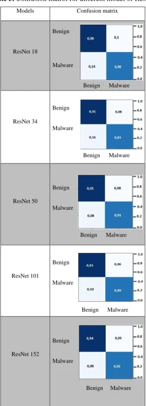
[Table 5] shows the confusion matrix successively of ResNet 18, ResNet 34, ResNet 50, ResNet 101 and ResNet 152.

We generate ROC curve of ResNet 152. In order to analyze this ROC curve, we must measure the area under curve (AUC) value. That helps us to know if our model ResNet 152 has the ability to differentiate between classes. In our case, we get AUC=0,94. It is a high value. That means our model (ResNet 152) is accurately predicting benign samples as benign and malicious samples as malicious.

Model FPR TPR

ResNet 18 0,14 0,90

ResNet 34 0,16 0,910

ResNet 50 0,08 0,91

ResNet 101 0,10 0,93

Table 5. Confusion matrix for different model of ResNet

Models Confusion matrix

ResNet 18

Benign

Malware

Benign Malware

ResNet 34

Benign

Malware

Benign Malware

ResNet 50

Benign

Malware

Benign Malware

ResNet 101

Benign

Malware

Benign Malware

ResNet 152

Benign

Malware

Benign Malware

So, the best performing model is the ResNet 152 model because it has the higher precision scores which involve both TP and FP values, in other words, with an AUC of 0.94, ResNet 152 is arguably a good model for our system [Fig 12].

For our system, we are going to go with ResNet-152 which is the most efficient one for our system with an accuracy value of 93,52%(We tested all the ResNet architectures: 18,34,50, 101 and152) [Fig13].

As we can observe in the[Fig14], the ResNet152 really performed better in terms of prediction accuracy. However, it performed poorly in terms of running time on malware dataset as compared with the other architectures (ResNet 18,

34, 50 and 101). But in our case, this difference of running time is not too remarkable that is why we accepted it.

Figure 12. Receiver Operating characteristic (ROC)

Figure 13. Comparison of ResNet models

0:37 0:40 0:43 0:51

0:56

Running Time (s)

Figure 14. Running time of different architectures of ResNet

As can be seen from the [Table6], we used 5 parameters in order to perform the prediction of malware. The role of every parameter is explained below.

• Poch: Denotes the number of iterations or passes of the entire training dataset.

• Train loss: Loss function output for the training set for that particular epoch. The loss function for our case is binary-cross entropy loss function.

• Valid loss: Same as train loss but on the validation / test set. For this experiment, validation set is same as test set as there is no hyperparameter tuning done

• Testing Accuracy: Represents a test method is said to be accurate when it measures what it is supposed to measure. This is calculated after every epoch.

• Time (second): time taken to train for the current epoch or iteration.

As we can see in the [Table6], the best accuracy to our system is 91,66%. However, we are not sure about this value. So, there is a simple way that can help us to determinate the reasonable minimum and maximum boundary value, this tool is “LR range test”. This test is reliable whenever having a new architecture dataset. Therefore, all we must do is to run our system for several epochs while the learning rate increase and decrease linearly between minimum and maximum LR value [Fig 15][24].

Table6. Model ResNet 152 before LR range test

Epoch Testing

Accuracy Train_loss Valid_loss Time

0 0,824074 0,627386 0,721273 00 :57

1 0,888889 0,447629 0,320702 00 :57

2 0,916667 0,318618 0,262 00 :56

3 0,907407 0,344537 0,495571 00 :56

0,10 0,12 0,14 0,16 0,18 0,20 0,22 0,24 0,26 0,28 0,30

le-06

le-05

le-04

le-03

le-02

LR

Figure 15. Learning rate plot

The main parameter that can change all the results in terms of increasing the accuracy and decreasing the error at a time, is the Epoch that indicates the number of times you browse the entire dataset.

We tested several different numbers of iterations of dataset using the LR range test and we get the following output. For the epoch 0 and 1, we can see the accuracy increases as the number of epochs rises. In which the testing accuracy of the epoch 0 was 87,96% and it increased to 90,74% in the epoch 1 [Table7].

For the two epochs 2 and 3, the value of testing accuracy is constant in the same percentage (93,52%). This step is the points that warns us and determines the number of epoch necessary to detect the malware. Therefore, in each operation of detection of malware, we must increase the epoch (the testing accuracy increases too) until the value of the accuracy stays constant or begins to decrease. Here we have to stop increasing the epochs [Table7]. In this case, the epoch 2 was the optimal one that stabilizes the highest accuracy (93,52%). [Fig16]: shows the evolution of the Loss function and the accuracy as a function of the epoch numbers for ResNet 152.

Table7. Model ResNet 152 after LR range test

Epoch _Accuracy Testing Train_loss Valid_loss Time

0 0,87963 0,604314 0,257363 00 :57

1 0,907407 0,408414 0,181318 00:57

2 0,935185 0,309338 0,167167 00 :56

3 0,935185 0,26714 0,151349 00 :56

0,00 1,00 2,00

200 400 600 800 1000 1200

Valid Train

Figure 16. Training and validation loss of our system using ResNet152

In order to simplify the total overview and the interpretation, the results are displayed as graph with two main parameters: The epoch and the Testing Accuracy [Fig17].

0.85 0.86 0.87 0.88 0.89 0.90 0.91 0.92 0.93 0.94

0 1 _Accuracy 2 3

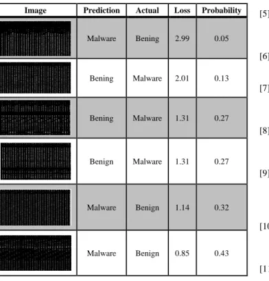
Figure 17. The optimal accuracy of ResNet15 Here are images of the output we got after running my code (Few images from the training dataset will be shown on 2 rows) [Table 18].

Deep learning provides an exceptional promising path towards, efficient, robust malware classification and detection.

After testing all architectures of ResNet model, our system performs better with 152 layers. However, this architecture is not the best one in terms of time. Despite of this ‘’negligible’’ difference, this note open a new door of a new research about finding a best model in terms of prediction accuracy and running time at a time.

Table 18. The images with maximum losses

7.

Conclusion

If we look at the trend of cyber security, we will find out that the whole world is looking forward to a solution to the ever-growing concern of malware. And thankfully deep learning and neural networks are showing new and promising hope. From regular articles to academic research papers, everyone is showing promising results.

The model we have presented here is relative simplicity and has shown its efficacy in the research that used it in this paper. In this work, we design a light-weighted deep learning-based malware detection system. Which has been proven to be capable enough to work well on different datasets. Furthermore, benefited from instruction grouping interpretation, the accuracy, and effectiveness of our method are all updated. Opposed to other work, our analysis, detection and prediction method is more lightweight both in aspects of the training data extraction and training time. In the future, our goal is to compare the difference between the methods of prediction, and we hope to achieve our goal so fast.

References

[1] J. E. Abdelkhalki, M. B. Ahmed, et A. Slimani, « Incident prediction through logging management and machine learning », in Proceedings of the 4th International Conference on Smart City Applications - SCA ’19, Casablanca, Morocco, 2019, p. 1‑8, doi: 10.1145/3368756.3369069.

[2] « Malware analysis », Wikipedia. févr. 29, 2020, Consulté le: mars 21, 2020. [En ligne]. Disponible sur: https://en.wikipedia.org/w/index.php?title=Malware_analysi s&oldid=943198641.

[3] J. Barriga et S. G. Yoo, « Malware Detection and Evasion with Machine Learning Techniques: A Survey », International Journal of Applied Engineering Research, vol. 12, p. 7207‑7214, sept. 2017.

[4] A. Chuvakin, K. Schmidt, et C. Phillips, Logging and Log Management: The Authoritative Guide to Understanding the

Concepts Surrounding Logging and Log Management. Newnes, p. 115‑135, mai 2012.

[5] M. Sebastián, R. Rivera, P. Kotzias, et J. Caballero, « AVclass: A Tool for Massive Malware Labeling », in Research in Attacks, Intrusions, and Defenses, Cham, 2016, p. 230‑253, doi: 10.1007/978-3-319-45719-2_11.

[6] K. Bartos, M. Sofka, et V. Franc, « Optimized Invariant Representation of Network Traffic for Detecting Unseen Malware Variants », p. 17.

[7] J. Z. Kolter et M. A. Maloof, « Learning to Detect and Classify Malicious Executables in the Wild », Journal of Machine Learning Research, vol. 7, no Dec, p. 2721‑2744, 2006.

[8] S. Chakraborty et L. Dey, « A rule based probabilistic technique for malware code detection », Multiagent and Grid Systems, vol. 12, no 4, p. 271‑286, janv. 2016, doi: 10.3233/MGS-160254.

[9] Z. Bazrafshan, H. Hashemi, S. M. H. Fard, et A. Hamzeh, « A survey on heuristic malware detection techniques », in The 5th Conference on Information and Knowledge Technology, shiraz, Iran, mai 2013, p. 113‑120, doi: 10.1109/IKT.2013.6620049.

[10] Y. Ki, E. Kim, et H. K. Kim, « A Novel Approach to Detect Malware Based on API Call Sequence Analysis », International Journal of Distributed Sensor Networks, vol. 11, no 6, p. 659101, juin 2015, doi: 10.1155/2015/659101. [11] S. Ren, K. He, R. Girshick, et J. Sun, « Faster R-CNN:

Towards Real-Time Object Detection with Region Proposal Networks », in Advances in Neural Information Processing Systems 28, C. Cortes, N. D. Lawrence, D. D. Lee, M. Sugiyama, et R. Garnett, Éd. Curran Associates, Inc., 2015, p. 91–99.

[12] A. Krizhevsky, I. Sutskever, et G. E. Hinton, « ImageNet classification with deep convolutional neural networks », Commun. ACM, vol. 60, no 6, p. 84‑90, mai 2017, doi: 10.1145/3065386.

[13] M. Furqan Rafique, M. Ali, A. Saeed Qureshi, A. Khan, et A. Majid Mirza, « Malware Classification using Deep Learning based Feature Extraction and Wrapper based Feature Selection Technique », arXiv e-prints, vol. 1910, p. arXiv:1910.10958, oct. 2019.

[14] R. Vinayakumar, M. Alazab, K. P. Soman, P. Poornachandran, et S. Venkatraman, « Robust Intelligent Malware Detection Using Deep Learning », IEEE Access, vol. 7, p. 46717‑46738, 2019, doi: 10.1109/ACCESS.2019.2906934.

[15] X. Glorot, A. Bordes, et Y. Bengio, « Deep Sparse Rectifier Neural Networks », p. 9.

[16] S. Dube, « Deep Learning for Malware Classification », Medium, mars 28, 2019. https://medium.com/ai-ml-at-

symantec/deep-learning-for-malware-classification-dc9d7712528f (consulté le mars 22, 2020).

[17] T. N. Sainath, O. Vinyals, A. Senior, et H. Sak, « Convolutional, Long Short-Term Memory, fully connected Deep Neural Networks », in 2015 IEEE International Conference on Acoustics, Speech and Signal Processing (ICASSP), South Brisbane, Queensland, Australia, avr. 2015, p. 4580‑4584, doi: 10.1109/ICASSP.2015.7178838. [18] M. Kalash, M. Rochan, N. Mohammed, N. D. B. Bruce, Y.

Wang, et F. Iqbal, « Malware Classification with Deep Convolutional Neural Networks », in 2018 9th IFIP International Conference on New Technologies, Mobility and Security (NTMS), Paris, févr. 2018, p. 1‑5, doi: 10.1109/NTMS.2018.8328749.

[19] S. Kornblith, J. Shlens, et Q. V. Le, « Do Better ImageNet Models Transfer Better? », arXiv:1805.08974 [cs, stat], juin 2019, Consulté le: avr. 18, 2020. [En ligne]. Disponible sur: http://arxiv.org/abs/1805.08974.

[20] L. Sun, « ResNet on Tiny ImageNet », p. 1 ‑6, avr. 2017.

Image Prediction Actual Loss Probability

Malware Bening 2.99 0.05

Bening Malware 2.01 0.13

Bening Malware 1.31 0.27

Benign Malware 1.31 0.27

Malware Benign 1.14 0.32

[21] chm, « Understanding and Implementing Architectures of ResNet and ResNeXt for state-of-the-art Image… », mc.ai, p. 2‑8, févr. 07, 2018.

[22] R. U. Khan, X. Zhang, et R. Kumar, « Analysis of ResNet and GoogleNet models for malware detection », J Comput Virol Hack Tech, vol. 15, no 1, p. 29‑37, mars 2019, doi: 10.1007/s11416-018-0324-z.

[23] S. Banescu, C. Collberg, et A. Pretschner, « Predicting the Resilience of Obfuscated Code Against Symbolic Execution Attacks via Machine Learning », p. 19.

[24] J. Howard et S. Gugger, « fastai: A Layered API for Deep Learning », Information, vol. 11, no 2, p. 108, févr. 2020, doi: 10.3390/info11020108.

[25] A. McDole, M. Abdelsalam, M. Gupta, et S. Mittal, « Analyzing CNN Based Behavioural Malware Detection Techniques on Cloud IaaS », p. 2 ‑16, févr. 2020.