Adoption Features and Approach for UWB Wireless
Sensor Network based on Pilot Signal assisted MAC
Kamran Ayub
1, 2, Valerijs Zagurskis
21
Technology Group, NYUAD Saadiyat Campus New York University. 2
Institute of Electronics and Computer Science, Riga Technical University, Latvia. [email protected], [email protected]
Abstract: In the field of wireless sensor network (WSN), Pilot Assisted Transmission (PAT) is a new concept. In our previous research, a mac layer algorithm called, “PA-MAC” was designed, which exclusively uses PAT technique for the medium access control. The performance of PA-MAC was evaluated under multi-hop and single multi-hop WSNs. It was excellent under a single multi-hop structure (i.e. network with a few nodes). But when it was evaluated for the dense network topology, the performance seriously declined. It was noted that the two main reasons of performance degradation are interference and transmission range. Technically there are two ways to tackle a dense network traffic problem. One is to use the multi-hop structure and the other one is clustering. In this research paper, clustering based adoption strategy is examined, and beside dynamic clustering approach multiple optimization features (i.e., clustering formation based on transmission range, dynamic cluster head selection and use of the Volterra code for the mitigation of interference) are added and tested. Collectively these adoption features have not only improved the media access performance but also optimized the network lifetime.
Keywords: Clustering, Energy efficiency, Media Access Control, Ultra wide band, Wireless Sensor Network.
1.
Introduction
PAT is a new concept in the field of wireless sensor network communication, due to its unique signal transmission structure, it has shown tremendous results when used for the mac layer in wireless sensor network. Earlier we had proposed one of the first medium access control algorithm “PA-MAC” based on PAT technique. That is, a schedule based MAC algorithm that uses impulse radio at the physical layer.
One of the main job of a sensor network is to securely and smoothly transfer the sensed data to the sink. This can be achieved only if the underneath network formation is correct (i.e., cluster is properly formed). The root cause of performance degradation in a PA-MAC architecture is its nodes formation in a heavy network topology. The traditional clustering and optimization procedures could not resolve the performance issues [2], because of Transmitted Reference/Delay Hopped Impulse Radio (TR/DH IR-UWB) at radio layer. In this research paper we have targeted these main performance degradation blockages and successfully optimized network performance by applying multiple adoption features. The improved architecture focuses the transmission range and node formation and uses (the same) pilot signal assisted mac with impulse radio at Physical layer. Due to the complexities involved in a multi-hop technique clustering approach for the network formation is used here. It is known that when the number of clients increases in a WSN cluster the whole burden comes on the MAC layer [3],
as a result collision and interference issues occur. Similarly selection of Cluster Head based (only) on residual energy can save the power but can create transmission and formation issues. As a solution for these challenges, our cluster formation is based on a transmission range rule, where groups are formed based on transmission range from the base station. Additionally, a threshold level is fixed for the cluster membership and the number of members for a cluster never crosses that limit. Beside this cluster head selection is based on multiple parameters called cost function. That selects the strongest node as cluster head. These two major enhancements not only simplifies the network formation but also improves the overall network performance. The rest of the research paper is divided as follows. Section 2 gives a brief overview of PA-MAC media access control algorithm. In section 3, a brief explanation of radio layer (Delay Hopped Transmitted Reference Scheme) is defined. Section 4 covers the clustering and proposed adoption features. In section 5 the network performance & simulation results are evaluated. The summary and conclusion are explained in Section 6.
2.
Media Access Control Layer
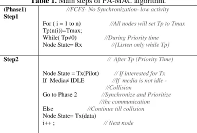
Use of PAT in WSN saves receiver’s energy and avoids channel estimation that is very attractive for the wireless sensor network [1], [2]. The main design of PA-MAC is based on two phases. Phase-1 is an initial phase which remains active unless the media access requests cross the threshold level. Right after the 1st collision (due to media access requests) control transfers to Phase-2. Phase 2 deals with different bottlenecks through prioritization and scheduling. See table 1 based on main steps of PA-MAC algorithm [1].
Table 1. Main steps of PA-MAC algorithm.
(Phase1) Step1
//FCFS- No Synchronization- low activity
For ( i = 1 to n) //All nodes will set Tp to Tmax
Tp(n(i))=Tmax;
While( Tp≠0) //During Priority time
Node State= Rx //{Listen only while Tp}
Step2 // After Tp (Priority Time)
Node State = Tx(Pilot) // If interested for Tx
If Media≠ IDLE //If media is not idle - //Collision
Go to Phase 2 //Synchronize and Prioritize //the communication
Else //Continue till collision Node State= Tx(data)
41 International Journal of Communication Networks and Information Security (IJCNIS) Vol. 8, No. 1, April 2016
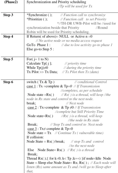
(Phase2) Synchronization and Priority scheduling
//Tp will be used for Tx
Step 3 *Synchronize ( ); // Function call to synchronize
*Prioritize ( ); // Function call to set Priority
*//TH-DR UWB-Pilot will be //used for synchronization beside that Priority //Round Robin will be used for Priority scheduling.
Step 4 If Return( of above)= NULL or Active n =0
// No active node or no media access request
GoTo Phase 1 : // due to low activity go-to phase 1
Else go-to Step 5 :
Step 5 For( j= 1 to N)
Calculate Tp[ j ]; // priority time
While Tp(j)≠0 // during the priority time
Tx Pilot >> Tx Data; // Tx Pilot then Tx (data)
Step 6 switch ( Tx & Tp ) // conditional Control
case 1 : Tx =complete & Tp=0 // If Transmission //completes, as per schedule
Node state =Rx( ) // Rx( ) is a thread, will keep //the node in Rx state and control to the next node.
break; // Next node
case 2 : Tx=complete & Tp ≠0 // If Transmission //complete but Still Priority Time
Node state=Rx( ) //Rx( ) is a thread, will keep //the node in Rx state
Break; // Stop Tx and control to Next node
case 3 : Tx≠ complete & Tp=0
Node state = Tx // Continue Tx ( vulnerable time)
If collision:
Node State = Rx( ) break; // stop Tx and control //to the next node
Else Node State= Rx( ) // Rx( ) is a thread
Break;
Thread Rx( );{ for k=0; k< Tp ;k++) }if node=Idle Node State = Sleep else Node State= Rx; Rx( ) ; // Each node will listen (Rx) same amount as Tx and //will go to Sleep after that,
The priority strategy in this algorithm is based on the following principles.
• The nodes that have completed their (access) time slot, and don’t have any more data, will not be considered for the next (priority) polling.
• After the completion of a (priority) schedule, the cluster head will create a new schedule by collecting access requests and once the priority schedule is finalized and shared with the member nodes. No new request will be accommodated for that cycle. Nodes with new access request will have to wait for the next schedule.
• During the new priority schedule design, the privilege will be given to the nodes who could not complete their turn in the previous round. If the time of arrival (of two or more than two nodes) is same, priority will be decided on the “shortest job first” rule.
At the end of each schedule, if there is no access request (in response to a pilot signal from CH). Phase 2 will be deactivated and control will transfer to Phase 1.
TRDH does not require channel estimation [5]. It gives very accurate synchronization and accumulates multipath energy very efficiently. See Figure1 for the TRDH pilot pulse design.
3.
Radio Layer Architecture
PA-MAC algorithm was tested with multiple receiver type (e.g. RAKE), but it works best with Transmitted Reference Delay Hoped (TRDH) receiver architecture [2]. TRDH consumes less energy than any other scheme when used for
Impulse Radio. This is because Impulse radio with TRDH does not require channel estimation [5], [10]. It gives very accurate synchronization, and accumulates multipath energy very efficiently. See Figure 1 for the TRDH pilot pulse design. As described in [2], radio layer uses a pair of pulses (doublet) instead of single pulse Figure 1. The first pulse (pilot signal) does not carry any data and is delayed (by a code) at the receiving node and works as a correlation pilot (reference) for the next pulse. Data/information is carried by the 2nd pulse of the pair (the doublet). Multiple access model can be achieved by adding the Volterra generated [8] delay code to each user. Here signal receivers are based on Delay Hoped energy detection design. That works asynchronously with power level 5-16 dBm for 5.4 GHz. Where radio dissipates Elec = 5.0 Nano Joule/bit, for a 1 Mbps data stream. IR-UWB Transmitter achieves pulse duration of 5 ns for the bandwidth of 500 MHz and consumes 250 Pico Jules/bit energy at 1 Mbps. PA-MAC algorithm’s duty cycling (scheduling) saves energy by turning the radio in sleep mode.
Figure 1. Delay Hoped Transmitted Reference UWB Scheme
4.
Proposed Strategy
In the traditional clustering approach, clusters are formed before the selection of cluster head [9], [10]. In the traditional way based on the residual energy (or any other factor), cluster head is selected. Cluster head selection is a significant step in network formation, and it has a huge impact on overall network stability [6]. Here a slightly different technique is introduced and cluster formation has been divided into two major parts. In this technique, adoption is divided into two parts; Formation-phase and Stabilize-phase. Formation phase focuses on cluster setup and CH selection, whereas data transmission and routing are managed in stabilize-phase.
Following are the major steps (with some assumptions). • Nodes are deployed randomly across the target region. • At the start of the simulation, all nodes have the same
amount of energy.
• All nodes have the ability to transfer data to any other node or to the BS (base station) using power control. • IR-UWB is used at radio layer. Channel characteristics
are symmetric (transmission power for a message from the x node to the y, (x→ y) node is same as (y→ x). 4.1 Formation Phase:
Cluster Formation & CH Selection: In the cluster formation segment, nodes are divided into groups based on their transmission range from the base station. To limit the number of nodes; a threshold level is defined. CH will not
doublet
1 Frame/Chip Tc = Tf
C1=
1 C2=-1
D1
exceed the membership of nodes (as described by threshold level). Following are thigh level steps.
• ‘n’ nodes are randomly deployed in the designated region.
• At start up, the base station (by using the pilot signal) collects the information of all the nodes.
• On reception of the pilot, every active node; sends the basic details such as node id, energy level and distance to the base station.
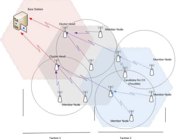
• Based on the received data, factions or groups are derived Figure 2. Accordingly CH is selected from the available candidates.
Here each faction is based on the transmission range from the BS. (e.g., nodes within base station’s Tx range are Faction 1) and faraway nodes are defined in higher level (e.g. Faction 2) and so on.
(CH selection is the first step, keeping the threshold limit each CH defines it cluster membership and forms clusters.)
After the selection of Cluster Head (CH uses pilot signal assisted MAC algorithm). Cluster head creates the schedule and shares with the member nodes. Once scheduled time-slot is assigned to the member nodes, following core steps are performed.
1. Data sensing process starts.
2. Based on the activity when data is sensed and gathered the nodes wait for their turn and transmit data to CH (according to defined MAC schedule [1].
3. At the end of each cycle, CH (cluster head) performs aggregation process and transfers data to the base station. Transmission from cluster head to base station could take direct or indirect via other cluster head route (depends on the routing strategy.
Explanation
In a common clustering approach, CH is nominated based on distance or residual energy [3]. Here we have used slightly different cluster head selection techniques. In our technique, each node selects CH first. Which is based on the cost function (cost function was explained in [4] which takes into account not only the energy level but also distance). To keep the size of cluster stable, a threshold level is applied to control the cluster membership. In this approach threshold level is calculated as simple as 10% of total nodes. Cost function [4] is used for the selection of cluster head.
= +
(1)
Here ‘T’ is distance (BS represents base station, Tmax is the maximum range). Based on the cost theory, other nodes (who have not selected CH) will select cluster head from the available candidates (of CH). The principle behind the cluster formation is based on the following formula.
= +
(2)
At the higher level, once CH is selected, nodes with lower cost are ignored. In this approach member nodes (of a cluster) are limited as per the threshold value that stables the cluster communication and increases the CH lifetime (as well as network). Right after the schedule sharing (with member nodes), the formation phase is considered complete and the stabilize phase (or data transmission phase) starts.
43 International Journal of Communication Networks and Information Security (IJCNIS) Vol. 8, No. 1, April 2016
4.2 Stabilize Phase
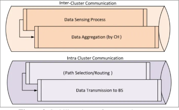
After the two main steps of network clustering, Cluster formation, and CH selection, the network is ready for its operations. This phase is called stabilize phase. During this phase, each cluster manages its data gathering and routing schedule by using MAC algorithm [1]. Stabilize phase carries two important communications, communication within the cluster, and communication with the sink (& other CHs). Figure 3 explains the design of stabilizing phase of our proposed method. In order to avoid the interference between these two communications, different channels are allocated to each cluster. That is shared with the member nodes of each cluster by CH. CH is updated with channel information from BS during formation phase.
4.2.1 Intra-Cluster Communication:
After the cluster formation and CH selection, member nodes collect data, and according to the mac-schedule forward it to the cluster head. Cluster head assembles (collected) data and performs aggregation. At the end of this step, data is forwarded to the base station (via neighboring cluster head or direct to BS) see Figure 2, Figure 3. All members of clusters use a unique channel number which is shared via CH. This protects the interference from neighboring cluster.
4.2.2 Inter-Cluster Communication
Each cluster head designs the communication schedule based on the Pilot signal Assisted-MAC, it is a multi-phase algorithm explained in [1]. See Figure 4 showing both types of communications with the logical paths. CH to CH communication or CH to BS communication uses a separate channel (different from the inter-cluster communication channel) which does not interfere with the inter-cluster communication.
Figure 3. Stabilize phase of proposed strategy
4.2.3 Interference Management
Due to the design nature of cluster-based architecture, interference is a common issue. Primarily interference is due to the nearby communication of adjacent cluster or coexisting communication among cluster heads. It can be dealt on multiple layers, normally on the physical layer and link layer. Here, the common interference issue, ‘Near-Far effect’ is managed by two-step inference management, where radio/physical layer thoroughly described in publication, and the MAC Layer both works together. This cross-layer structure creates communication stability and avoids interference. Addition to this for the inter-cluster communication interference, the coding technique the
Volterra Model [8] protects the communication from internal interference. As discussed as each cluster head uses a different channel for its internal communication, which is shared by CH with members. Once a node leaves a cluster, or when cluster ends its life, all affected members get default channel. This remains their default communication channel until a new cluster is formed or they join a cluster. Besides this, proposed model is centrally coordinated and synchronization is well controlled by ‘Transmitted Reference’ scheme see Figure 1.
Table 2. Simulation parameters and corresponding values
Parameters Values
Network Area (m) 100x100
No. of Nodes (n) 100
Initial Energy (of nodes) 1 J
5 nJ/b
Datagram 4 Kbits
Pulse Duration 5 ns
No of Runs 50
250 pJ/b
D 50m
5.
Simulations & Performance Evaluation
Starting with the experimental design and performance matrices. MixiM (under OMNET++) for the overall modeling is used. For optimization analysis, MATLAB is used. For the Radio layer same structure defined in [2] is used, it was thoroughly tested under MATLAB in our last publication [2].
Table 2 shows the core parameters and their values used in the simulation.
5.1 Average Energy
One of the way to check the effectiveness of optimization technique is to calculate the average energy consumption for multiple rounds, if outcome comes as less energy consumption that means optimization worked. Using the same rule, OCT is evaluated. Here for the energy consumption of the transmutation of an x-bit formula is derived from [3].
=
+
(3) E is the total energy consumed at the node ‘i'. E ! is the energy consumed at the transmitter end and it’s given by", $ =
%&%'× " + )*
+,× " × $
-.
(4)
Similarly E/! is receiver’s consumption and its equal to
" =
%&%'× "
(5) E0102 is the expended energy (of radio) and it is assumed that
Figure 4.
In simulation, when the battery life of a node depletes to “zero” it is considered dead. To make it more realistic, a random function is used for this purpose.
Over here scenarios are applied and simulation is executed for 50 runs. The network size is 100X100 m. As the aim of this research is to examine the performance under dense or heavy traffic, numbers of nodes are kept same for all the scenarios (i.e. n= 2 to 100 in all scenarios), value of ‘n’ gradually increases, that gives more clear understanding about the network performance in dense cases. Results are validated by comparing with famous LEACH protocol the same way author examined in [7].
In the first scenario value of n is kept constant to
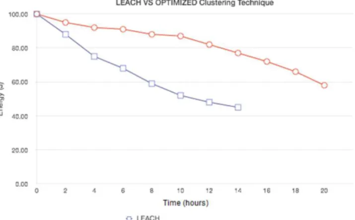
the simulation results Figure 5, it can be seen that optimized clustering technique’s residual energy is improved even in a dense network case (n=100). Comparing the remaining energy of LEACH and OCT, one can see that, after the 14th hour; for the same number of nodes Leach has about 40 Jules (residual energy), on the other hand OCT has about 75 Jules. OCT excels in both energy and packet delivery. There are many success factors behind this optimization, cross coordination, synchronization, interference management and CH selection technique are the major once. Moreover, in OCT there is no channel estimation involved that saves transceiver energy.
Figure 4. Intra & Inter-Cluster Communication
In simulation, when the battery life of a node depletes to “zero” it is considered dead. To make it more realistic, a imulation is executed for 50 runs. The network size is 100X100 m. As the aim of this research is to examine the performance under dense or heavy traffic, numbers of nodes are kept same for all the scenarios (i.e. n= 2 to 100 in all scenarios), value of ‘n’ gradually increases, that gives more clear understanding about the network performance in dense cases. Results are validated by comparing with famous LEACH protocol the In the first scenario value of n is kept constant to 100. From the simulation results Figure 5, it can be seen that optimized-clustering technique’s residual energy is improved even in a dense network case (n=100). Comparing the remaining energy of LEACH and OCT, one can see that, after the 14th he same number of nodes Leach has about 40 Jules (residual energy), on the other hand OCT has about 75 Jules. OCT excels in both energy and packet delivery. There are many success factors behind this optimization, cross-layer interference management and CH selection technique are the major once. Moreover, in OCT there is no channel estimation involved that saves
5.2 Lifetime of the Network
The lifetime of a network is directly proportional to the lifetime of its nodes. Which in fact depends on the succession of packet delivery.
Network life time is calculated as the time before its first node goes down. As our aim is to check the complete performance, we used a slightly different appr
formula for network life time is basically on the rule “The time before the last node
Figure 5. Energy Consumption (LEACH vs. OCT) Lifetime of the Network
The lifetime of a network is directly proportional to the its nodes. Which in fact depends on the succession of packet delivery. In conventional approach Network life time is calculated as the time before its first node goes down. As our aim is to check the complete performance, we used a slightly different approach and our formula for network life time is basically on the rule “The
International Journal of Communication Networks and Information Security (IJCNIS)
goes down and where there is some network activity in process.
Increase number of jamming during data transm
packet drop during a session can put repetitive burden on the network flow that consumes lots of additional energy. Similarly death of node also effects overall network performance.
During the 2nd scenario, network size is gradually increased (n=5 nodes to n=100).
It is observed that the network lifetime remains between 6 and 9 hours (which is very stable figure). By increasing the number of nodes, life time of network also increases. Technically that is true because energy burden is divided among nodes. Looking at the graph, network lifetime was on its peak when n=100. Which is biggest “n” value.
Figure 6. Network Life-Time Analysis
That means OCT has resolved the issue (Pilot assisted MAC performance under dense network) where network performance drops when n > 20. From simulation analysis, OCT gives same level of performance as LEACH.
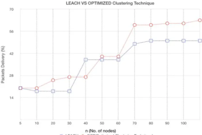
Figure 7. Packet Success delivery Ratio
Just to make sure that results are accurate, experiments are repeated multiple times. Most of the times it is observed that optimized clustering technique has better results (a few both have same results, and that is natural and acceptable in simulation environment). The optimized clustering scheme has smooth performance in case of network lifetime see Figure 6. One of the reasons; why optimization technique provides smooth results is due to the use of cost function. Where not only energy but also other factors a considered.
nal Journal of Communication Networks and Information Security (IJCNIS)
goes down and where there is some network activity in mming during data transmission or packet drop during a session can put repetitive burden on the network flow that consumes lots of additional energy. effects overall network network size is gradually increased It is observed that the network lifetime remains between 6 and 9 hours (which is very stable figure). By increasing the number of nodes, life time of network also increases. Technically that is true because energy burden is divided ong nodes. Looking at the graph, network lifetime was on its peak when n=100. Which is biggest “n” value.
Time Analysis 1
OCT has resolved the issue (Pilot assisted MAC performance under dense network) where network performance drops when n > 20. From simulation analysis, OCT gives same level of performance as LEACH.
Packet Success delivery Ratio
sure that results are accurate, experiments are repeated multiple times. Most of the times it is observed that optimized clustering technique has better results (a few times both have same results, and that is natural and acceptable in nt). The optimized clustering scheme has smooth performance in case of network lifetime see Figure 6. One of the reasons; why optimization technique provides smooth results is due to the use of cost function. Where not only energy but also other factors are also
5.3 Packet Delivery Ratio
Another way to judge the performance of optimization changes is to examine the successful packet delivery ratio. The fundamental formula for this is
“Percentage of successfully transported packets = Total No. of Received packets/Total No. of Transmitted packet
From Figure 7, 8, it is observed that the optimized clustering approach has better packet delivery value than LEACH. Performance remains consistent even when the number of nodes are gradually increased
ups and downs in the graph that shows the death of a node during simulation (which works in random fashion). Overall it proves the success of PA
environment. It is also observed that as the number of nod increases, the packet delivery improves. This is because more nodes mean more options of routes with BS and more candidates for the cluster head. From Figure 8, we can observe
That more packets arrived on the base station when optimization techniques (e.g. OCT) is used
Figure 8. Packet Reception at BS (percen
Conclusion
Pilot assisted Medium Access control (PA
“PAT” (pilot assisted transmission) based MAC algorithm specifically designed for the wireless sensor network. Due to its remarkable performance in WSN, after the
of algorithm as next step we decided to define a complete framework. A part of our framework design, this research was focused on the optimization and multiple adoption. In this paper we targeted those issues due to them PA was failed in the dense deployment. Our results p
using transmission range based adoption features has not only resolved the old issues (e.g. Packet delivery performance, Network life time etc.) but has some additional advantages over the conventional MAC protocols e.g. it’s only WSN protocol which provides cross layer compatibility between Radio (UWB) and MAC. Though when PA was used in a dense network environment. in our previous research, due to the weak topology, it‘s performance in terms of packet delivery, energy consumpti
was degraded. We investigated these issues and noticed that the two main reasons are topology and weak routing structure. In this paper, in our strategy, selection of cluster head is based on a cost function. That considers multiple properties e.g. transmission ranges, residual energy provides a better choice for cluster management and keeps the cluster structure balanced. Clustering based on 45 Vol. 8, No. 1, April 2016
Packet Delivery Ratio
Another way to judge the performance of optimization changes is to examine the successful packet delivery ratio. The fundamental formula for this is,
Percentage of successfully transported packets = Total No. of Received packets/Total No. of Transmitted packet”
From Figure 7, 8, it is observed that the optimized clustering approach has better packet delivery value than LEACH. Performance remains consistent even when the number of nodes are gradually increased .e.g. n=100). There are some ups and downs in the graph that shows the death of a node during simulation (which works in random fashion). Overall it proves the success of PA-MAC in a dense network environment. It is also observed that as the number of nodes increases, the packet delivery improves. This is because nodes mean more options of routes with BS and more candidates for the cluster head. From Figure 8, we can more packets arrived on the base station when
e.g. OCT) is used
Packet Reception at BS (percentage)
transmission range gives a stable as well as control cluster heads mechanism, which prevents packet drop, interface management and media access management Simulation results show that our optimization technique has improved the performance of PA-MAC even in a dense network environment. Consolidated results with LEACH verify, that in most of the cases optimized clustering technique has better performance than LEACH. Performance is also compared with the pre-adoption state of the framework and found very positive results. In future, we have a plan to deeply investigate its self-organization feature
References
[1] Kamran Ayub, V. Zagurskis, “IR-UWB Radio Architecture for Wireless Sensor Network Based on Pilot Signal Assisted MAC”. 6th International Conference on New Technologies, Mobility & Security (NTMS), ISBN: 9781479932238, pp. 1-5, 2014.
[2] Ayub K, Valerijs. Z, “Pilot signal assisted Ultra-Wideband medium access control algorithm for Wireless Sensor Networks”. Telecommunications Forum (TELFOR) 21st Conference Belgrade. ISBN: 978-1-4799-1419-7, 2013. [3] V. J. Mathews and G. L. Sicuranza. Polynomial Signal
Processing. Illustrated Edition. Chichester, England: John Wiley & Sons Ltd. 2000: 121-129.
[4] N. M. Abdul Latiff, C. C. Tsimenidis, B. S. Sharif. An Energy-aware Clustering Technique for Wireless Sensor Networks. IEEE 18th International Symposium on Personal, Indoor and Mobile Radio Communication PIMRC’07. September 2007 New Castle, UK; 1-5.
[5] H. Hoctor and H. Tomhon. An Overview of Delay-Hopped, Transmitted Reference RF communications. GE Technical Information Series Report, CRD 198, 2001/2002.
[6] Veena Bhat, Sharada U. Shenoy. Effective Cluster Head Selection Based on EDM for WSN. The IUP Journal of Computer Science, July 2014; Vol. 8, Issue 3, page 47. [7] Lu Tao, Zhu Qing-Xin, Zhang Luqiao. An Improvement for
LEACH Algorithm in Wireless Sensor Network. Industrial Electronics and Applications (ICIEA) Taichung, 2010, 1811-1814
[8] De-xuan ZOU, Li-qun GAO, Steven LI. Volterra filter modeling of a nonlinear discrete-time system based on a ranked differential evolution algorithm. Journal of Zhejiang University-Science 2014 15(8):687-696
[9] M. Hussaini, H. Bello-Salau, A. F. Salami, F. Anwar, A. H. Abdalla, Md. Rafiqul Islam, “Enhanced Clustering Routing Protocol for Power-Efficient Gathering in Wireless Sensor Network” International journal of communication networks and information security (IJCNIS), ISSN: 2076-0930, Vol 4, No. 1, 2012, pp. 18-28.