Physically-based sampling for motion planning

(1)

Physically-based Sampling for Motion Planning

Thomas Russell Gayle

A dissertation submitted to the faculty of the University of North Carolina at Chapel Hill in partial fulfillment of the requirements for the degree of Doctor of Philosophy in the Department of Computer Science.

Chapel Hill 2010

Approved by:

Dinesh Manocha, Advisor

Ming C. Lin, Reader

Patrick G. Xavier, Reader

Mark Foskey, Committee Member

(2)

c 2010

(3)

Abstract

Thomas Russell Gayle: Physically-based Sampling for Motion Planning. (Under the direction of Dinesh Manocha.)

Motion planning is a fundamental problem with applications in a wide variety of

areas including robotics, computer graphics, animation, virtual prototyping, medical

simulations, industrial simulations, and traffic planning. Despite being an active area

of research for nearly four decades, prior motion planning algorithms are unable to

provide adequate solutions that satisfy the constraints that arise in these applications.

We present a novel approach based on physics-based sampling for motion planning that

can compute collision-free paths while also satisfying many physical constraints. Our

planning algorithms use constrained simulation to generate samples which are biased

in the direction of the final goal positions of the agent or agents. The underlying

simulation core implicitly incorporates kinematics and dynamics of the robot or agent

as constraints or as part of the motion model itself. Thus, the resulting motion is smooth

and physically-plausible for both single robot and multi-robot planning.

We apply our approach to planning of deformable soft-body agents via the use of

graphics hardware accelerated interference queries. We highlight the approach with a

case study on pre-operative planning for liver chemoembolization. Next, we apply it to

the case of highly articulated serial chains. Through dynamic dimensionality reduction

and optimized collision response, we can successfully plan the motion of “snake-like”

robots in a practical amount of time despite the high number of degrees of freedom in

the problem. Finally, we show the use of the approach for a large number of bodies in

dynamic environments. By applying our approach to both global and local interactions

between agents, we can successfully plan for thousands of simple robots in real-world

(4)

(5)

Acknowledgments

When I first walked onto the campus at the University of North Carolina, I remember

thinking it would be a great place for me to take the next step in my education. It certainly

was a great place for this, but I never could have imagined that it would have such a significant

impact on who I am and on my life today. The Department of Computer Science, the

Univer-sity, and even the town of Chapel Hill has been a wonderful and supportive environment. I met

some amazing people, and made some of my best and closest friends while working towards

my academic goals.

I really do feel fortunate to have had a great set of people supporting me over the years

and in my endeavors. I would like to extend a great amount of thanks to my advisor, Dinesh

Manocha. His support and persistence never faded, even through some fairly trying times. I

owe him a great amount of gratitude for his help, his advice, and his support of my work. I

could never have gotten this far without him, as both an individual and a researcher. I also

want to thank my co-advisor, Ming Lin, whose guidance helped me through many difficult

places and who always helped me reach out and network with the academic community. I

want to extend a special thanks to my committee members. Many thanks to Patrick Xavier

for being a collaborator and mentor during my summer at Sandia National Labs and for many

interesting discussions and useful feedback on my work. Also, many thanks to Mark Foskey

and Nancy Amato for their support and their feedback over the past few years.

I’m extremely thankful for the Department of Energy’s High Performance Computing

Fellowship, the Krell Institute, and its staff. The Fellowship and Krell opened my eyes to

many opportunities and a wealth of interesting research projects. The summer I spent at

Sandia National Laboratories was a wonderful experience and definitely helped to shape who

I am today and what I want to do in the future.

Over the years, it has been a joy and honor to have worked with such a motivated and

talented group of individuals. I owe a great deal of thanks to my co-authors Avneesh Sud,

(6)

Klingler, Stephane Redon, Stephen Guy, and William Moss. Without them, much of this work

may not have been possible or would have taken much longer. I’d like to thank the members of

the UNC GAMMA Research group for all the feedback, support, and interesting discussions.

I also want to thank many members of the Department of Computer Science staff, including

Sandra Neely, Missy Wood, and Janet Jones, for all their friendliness and support as well.

One of the greatest joys of my time in Chapel Hill has been all the great friends I have

made along the way. I’d like to thank two of my close friends in particular, Avneesh Sud and

Sasa Junuzovic. I will cherish the good discussions, late night coffee runs, and especially all

the fun times. To Karl Strohmaier, Jason Sewall, Sarah Kennedy, Vince Noel, Tynia Yang,

Brian and Carol Begnoche, Jeff Terrell, Keith Lee, Stephen Olivier, Aaron Block, Luv Kohli,

and Nico Galoppo, you all are some the best friends imaginable.

Many thanks go out to my parents, T. Vincent Gayle and Theresa Gayle, for their love,

their care, their support, and mostly for believing in me and allowing me to grow into the

person I am today.

Finally, to my wife Sarita I give my utmost gratitude for her love, her support and for

(7)

List of Tables

4.1 Deformable robot planning performance: This table highlights the performance of our planner running on a laptop with a 1.5GHz Pentium-4 processor. We highlight geometric complexity of the environment in terms of the number of triangles. We report the high-level path generation time and simulation time. The last column reports the average time taken per simulation step. . . 84

4.2 Planning performance with 2.5D overlap test: This table gives a breakdown of the average time step for each scenario. Constraint update refers to the time spent in computing each constraint for the given config-uration. The 2.5D overlap test along with the exact triangle intersection test are the two stages of the collision detection algorithm. The Solve-System time is that spent in solving the motion equations during each step. . . 93

5.1 Articulated body planning performance table: Planning perfor-mance breakdown across each of our benchmarks. Longer simulation times result from the robot having to travel a greater distance, whereas the average step times are relatively uniform across all environments. . . 127

6.1 Uniform Sampling vs. APSL in Roadmap Cleanup. This shows the reduction in input roadmap size based on the APSL sampling metric. 185

6.2 Planning times for benchmarks: This table shows the timing for each of our benchmarks. Forces (force computation, constraint updates), update (motion equation integration), and step time are averages over the entire planning run. Total time is the amount of time it took to find a planning solution. . . 187

(13)

List of Figures

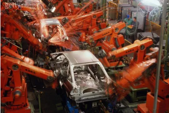
1.1 Car manufacturing plant, robotic assembly line, elevated view: Courtesy of Getty Images. http://www.gettyimages.com/detail/LA4074-003/Riser, 2009. . . 2

1.2 Trade show simulation: In the tradeshow scenario, each agent has a series of goals which it must visit. Realistic movements and interac-tions between humanoids is critical to creating a compelling and realistic simulation. . . 3

1.3 Workspace vs Configuration space: This planning situation requires the triangle to move translationally (no rotation) from the blue to the pink position. The left image contains the start and final configurations, while the right image maps it to its configuration space. The initial and final configurations can be represented as a point in C while theC−obstacles have been enlarged. Here, theF is the white area on the right image. . 6

1.4 Cell decomposition: A vertical cell decomposition of theC is computed by extending the vertices of theC obstacles vertically to the environment boundary. A path is created by connecting the midpoints of adjacent cells. 8

1.5 Roadmap: A roadmap is created by randomly sampling the C. Each sample in F is then connected to the nearest neighbors on the roadmap. To find a path, the initial and goal configurations are connected to the roadmap. Then, the shortest path between the configurations is found and used as the path. . . 9

1.6 Potential field: Since all obstacles here are given a repulsive or high potential value, this potential field path causes the robot to try to stay optimally far from obstacles as it navigates toward the goal. . . 11

1.7 Planning of a deformable cylinder: The final path of a deformable cylinder as it travels through a series of walls with holes. The cylinder’s radius is chosen so that it must deform in order to reach its goal. . . 26

(14)

1.9 Impact of multiple agents: The presence of multiple agents can greatly impact the realism of a scene or scenario. On the left, we see a scene with only the user’s avatar in an online virtual world. On the right, the avatar is joined by intelligent agents which can autonomously navigate the virtual world. . . 31

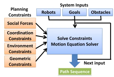
3.1 Planner Architecture: The physics-based motion planning cores uses the robots, goals, obstacles, and a set of planning constraints as its input. By solving the constraints (several different types are mentioned in the figure) and applying the resulting forces, motion is generated and the system is updated. The resulting value is a waypoint along the path and serves as the next input. . . 58

4.1 The Ball in Cup Scene: The goal is to plan a path to move the ball into the cup. Since the cup’s rim has about the same diameter as the ball, a deformation on the ball simplifies the path planning. The image, generated by our planner, shows the path of the deforming ball as it moves toward the center of the cup. Note that the final path causes the ball to deform around the rim of the cup. . . 68

4.2 Path Planning of Catheters in Liver Chemoembolization: The deformable catheter (robot), represented by 10K triangles, is 1.35mm in diameter and approximately 1,000mm in length. The obstacles including the arteries and liver consist of more than 83K triangles. The diameter of the arteries varies in the range 2.5-6mm. Our goal is to compute a collision free path from the start to end configuration for the deformable catheter. The free space of the robot is constrained. The path computed by our motion planner is shown in Fig. 4.9. . . 71

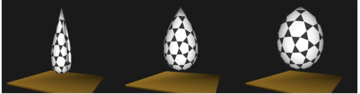
4.3 Soft-body robots with varying internal pressures: The leftmost robot has a relatively low pressure, while the rightmost has a fairly high pressure. The middle image has a pressure value in between the other two. 82

4.4 SphereWorld benchmark: The robot is shown in wireframe, and is deforming between some of the larger spheres. Each of the larger spheres are stationary, rigid obstacles. . . 83

(15)

4.6 Tunnel benchmark: This environment is a simple tunnel which the robot must travel through in order to reach the goal. In this image, the striped cylinders represent the deformable robot at various states in its path through the tunnel. Note that a collision-free would not be possible if this robot was not deformable . . . 85

4.7 2.5D overlap tests used for collision detection: The query checks whether there exists a separating surface along a view direction of depth complexity one. S has depth complexity more than one from View 1 as well as View 2. In the right image, s1 has depth complexity one from

View 1 ands2 has depth complexity one from View 2. As a result, we use

two 2.5D overlap tests to decide that R1 and R2 are not colliding with

the obstacles (Oi). . . 86 4.8 2.5D speed-up vs. triangle count: This graph highlights the speedups

obtained by utilizing the 2.5D overlap tests in our collision detection algorithm, as we increase the polygonal complexity of our scene. We observe nearly an order of magnitude improvement in complex scenes over prior algorithms based on bounding volume hierarchies. . . 94

4.9 Path Planning of Catheters in Liver Chemoembolization: We highlight the collision-free computed by our algorithm for the catheter shown in Fig. 4.2. We show the overall path from the start to the end configuration in the rightmost image. The left images highlight the zoomed portions of the path, showing bends and deformations. . . 96

5.1 Construction of an articulated body: An articulated body Ais con-nected to bodyBat the principal joint,j2, to form bodyC. The assembly

tree forC is shown beneath the body. Forces and accelerations which gov-ern C’s motion are shown. . . 100

5.2 Collision Frame: The collision frame, Fcoll is determine by the point of contact and the contact normal. By convention, thez-direction of the collision frame is in the direction of the contact normal. Forces upon link k must be transformed from the Fcoll toFk, the link’s inertial frame. . . 112

(16)

5.4 Pendulum benchmark: For testing the feasibility of our collision han-dling approach, in this benchmark an articulated pendulum with one end fixed to a point falls toward a set of randomly placed cylinders. The pen-dulum is modeled with 200 DOF. A visually accurate simulation was run with only 40 active DOFs and gives a 5X speedup in collision detection and response computation. . . 123

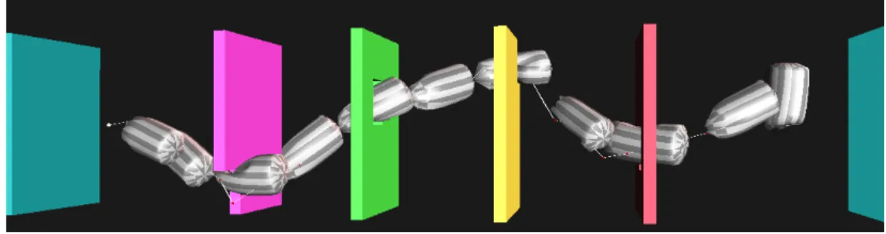
5.5 Threading benchmark: The articulated body is modeled with 300 DOFs and moves through a sequence of holes in walls. At each step of the simulation, we use only 60 DOFs for adaptive dynamics and collision response computation. Overall, our adaptive algorithm results in 5X speedup in this simulation. . . 123

5.6 Bridge benchmark: The articulated body travels around the bridge in a snake-like motion. The body contains over 500 links and 500 DOFs (i.e. 500 DOFs). We used only 70 DOFs for adaptive dynamics and collision response, resulting in 8X improvement in the simulation. . . 124

5.7 Collision response time vs. number of active joints: This chart shows the average time to process a collision for a fixed number of active joints. It also shows that there is a relatively linear relationship between the active joints and the running time. . . 125

5.8 Planning time vs. Number of active joints: Relationship between active joints and planning time for the Serial Walls (300 DoF) and Tunnel benchmarks (600 DoF). The horizontal line represents the time taken by using Featherstone’s DCA algorithm. The values above it are the speed-ups over the DCA algorithm when that many active joints are simulated.

. . . 128

5.9 Articulated planning benchmark scenarios: (a) Serial Walls; (b) Tunnel; (c) Liver Catheterization; (d) Pipes; (e) Debris. . . 129

5.10 Full vs. Reduced dimensionality articulated body accuracy: Vi-sual comparison of the simulation of an articulated with 100 joints. On the left, all 100 joints are simulated while on the left only the most im-portant25of the 100 are simulated. Each segment represents a rigidified portion of the body. . . 130

(17)

6.1 Guarding and escorting: This image is from a guarding and escorting scenario. 35 aggressive robots (in red) are trying to reach an important robot (in green). The black robots are attempting to stay in a formation while protecting the important robot. Their goal is to escort it across the environment. Our social force model allows the aggressive robot to move toward the important robot while avoiding collisions and distance coordination constraints are used to help maintain the formation. This benchmark took 132.9 s with an average step time of 42 ms. . . 136

6.2 Reactive Deforming Roadmaps (RDR): The RDR contains a set of dy-namic milestones and reactive links. Each of these are represented with

C-space particles: a point mass in the configuration space. As the obsta-cle oi moves, the dynamic milestones move as well and the reactive links

of the roadmap deform to avoid the obstacle boundary. (c) If a path link deforms too much or is too close to the obstacleoi, the link is removed. 141

6.3 Social Potential Fields: This figure compares Inverse-force laws (dark-blue and green curves) and Helbing’s social force laws (red and cyan curves) with differing parameters. The Inverse-force plots initially decline rapidly, and then the rate of decline slows greatly. On the other hand, the Helbing plots do not smoothen out quite as quickly and do not grow indefinitely as distance approaches 0. . . 144

6.4 Antipodal Robots: In this benchmark, 16 polygonal robots, colored by starting quadrant, start along the edge of a circle. Each robot must travel to a position across the circle and to a different orientation. This sequence shows four steps in the planning. (a) The robots are at their initial position. (b-c) The robots are in the process of moving across the circle, where social forces help prevent collision while also leading toward the anti-podal position. (d) The agents arrive at their anti-podal positions and we see the paths they traveled. . . 145

6.5 Adding links to the RDR: (Left) To explore, a random sample q1

rand

is generated, and its nearest neighbor to the roadmap is found, q1

near.

To merge different connected components, a random milestone, q2_rand on Component 2 is selected and its nearest neighbor on Component 1 is found, q2

near. (Right) New milestones, qnewi are added by extending qneari

towardq_randi and valid straight-line links are added. . . 146 6.6 Unsafe and Safe Link Samplings: (Left) The default sampling of

linkl1 is insufficient, since the safety region (circles) defined byη(p1) and

η(p2) do not overlap. Similar for linkl2. (Right) The addition of particles

p4 and p5 result in safe links, since the the entire link is covered by some

(18)

6.7 Adding and Removing Particles: (Left) The links, between orange circles as the endpoints, have been sampled based on the position of a dynamic obstacleO1. Samples are shown as green circles. The blue open

circles show the safety region for each particle (Middle) As O1 moves,

η(pi) is updated for each particle. As a result, there are redundant par-ticles on linkl1 and too few particles on linkl3. (Right) The add particle

procedure adaptively adds particles to l3 until it passes the safety

crite-rion, and particles who belong in the safety regions of its neighbors have been removed froml3. . . 152

6.8 Reactive Deforming Roadmaps (RDR): An example with 4 transla-tional agents (red circles) and goals (yellow triangles). The static obsta-cles shown as dark blue rectangles and dynamic obstaobsta-cles are shown as cyan rectangles with arrows indicating the direction of motion. The green curves represent links of the reacting deforming roadmap, using uniform sampling. The dynamic obstacles represent cars. As the highlighted car (circled) moves, the affected link in the roadmap is removed. . . 157

6.9 Roadmap Link Bands: Link bands are a partition of the freespace based on the links of RDR. (a) Several RDR links, in solid black lines, respond to a static obstacle, O2 and a dynamic obstacle O1. The link

band, B(1), for link l1 is shaded, and the link boundaries are shown as

dashed lines. (b) As O1 approaches link l2 it deforms. Link band B(1)’s

boundary is highlighted in bold dashed lines and shows the two segments of the milestone boundary,Bm(1), and the intermediate boundary Bi(1). (c) Linkl2 is removed due O1’s motion while the link band B(1) changes

to reflect the removal. . . 158

6.10 Social Force Discretization: Since the general social force integral is difficult to compute, we discretize the domain. This figure shows the discretized social force computation on ri from rj. Robot ri has been uniformly sampled into a set of points, shown as small blue dots. For each sample,pi_nwithin a fixed distance fromrj,Fsoc(pi_n, rj) will be computed. By the force law definition, points closer to rj such as pi15 will receive

larger forces than points farther away, such as pi

6. For points too far

(19)

6.11 College campus: (a) Many areas in online virtual worlds, such as this college campus in Second LifeR, are sparsely inhabited. (b) We present

techniques to add virtual agents and perform collision-free autonomous navigation. In this scene, the virtual agents navigate walkways, lead groups, or act as a member of a group. A snapshot from a simulation with 18 virtual agents (wearing blue-shaded shirts) that automatically navigate among human controlled agents (wearing orange shirts). (c) In a different scenario, a virtual tour guide leads virtual agents around the walkways among other virtual and a real agent. . . 164

6.12 Local Navigation via social forces: The colors of the arrows corre-spond to the specific object that generates the social force. (a) Agentr1

is acted upon by social repulsive force Fsoc

2 (r1) from r2, attractive force

Fatt

3 (r1) from r3, repulsive obstacle force Fobs1 (r1) from o1, and goal force

Fgoal(r1). Repulsive and attractive forces encourage the agent to move

toward or away from agents and obstacles, respectively. (b) An additional velocity bias force Fvel

2 (r1) is computed to account for agent r2’s velocity

during inaccurate sensing. By assuming a linear trajectory over a short period of time, we can help to reduce the impact of network latency. No velocity bias force is computed for r3 since it is heading in the same

di-rection asr1. The final net forceFnet(ri) reflects the sum of all the forces and serves as the agent’s next heading. . . 167

6.13 Multiple robots on the RDR: For proper avoidance, each robot ap-plies forces on the RDR except on the particles that are in its fixed particle zone. . . 170

6.14 Adding additional links between milestones: As the robot r2

ap-proaches a link occupied by r1, an additional link L2 is added for r2 to

traverse. . . 171

6.15 Agent clusters for fast proximity computation: (Left) Each color corresponds to a unique cluster of nearby agents. Link band boundaries are shown as dashed orange lines. (Center) Zoomed-in view of the clusters in the boxed region, with a single agent highlighted and circled. The roadmap force components are shown for another agent with the central milestone as next intermediate goal. nl denotes the unit normal vector from agent to the link l. ek denotes the unit vector direction towards next goal. (Right) Cluster updates are highlighted, as an agent crosses a link band boundary. . . 172

(20)

6.17 Maze environment: Left: Navigation of 500 virtual agents in a maze consisting of 8 entrance and 8 exit points. Center: Each agent computes an independent path to the nearest exit using adaptive roadmaps. Right: Our local dynamics simulation framework based on link bands captures emergent behavior of real crowds, such as forming lanes. We perform real-time navigation of 500 agents at over 200fps. . . 178

6.18 Multi-robot motion planning of 15 star-shaped robots in differ-ent colors using reactive-deforming roadmaps: (a) Initial configu-ration. Each robot has 3-DOF (2T+R) and acts as a dynamic obstacle for the other 14 robots. The goal for each robot is represented as a thick point of same color. Thin gray segments represent the initial roadmap, thick colored segments denote the path for each robot. (b)-(c) Two timesteps of our planning algorithm. Only the deforming paths are shown. (d) The final configuration showing the reactive-deforming roadmaps and the cor-responding paths. Total number of simulation steps = 1,525, average time per step = 10.6 msec on a 2.1GHz Pentium Core2 CPU. . . 181

6.19 Application of N-body motion planning using reactive deform-ing roadmaps to complex crowd simulation with human agents and polygonal dynamic obstacles: (a)-(b) An instructive example with 4 agents (in red) and goals (in yellow). The static obstacles are in dark blue and dynamic obstacles (cyan). The reactive deforming roadmap is shown with green links. The dynamic obstacles represent cars. As the highlighted car (circled) moves, the affected link in the roadmap is re-moved. (c) A real-time simulation of motion planning for 100 human agents and 4 cars in same environment. The average time for roadmap update and motion planning per frame = 11.5ms on a 2.1Ghz Pentium Core2 CPU. . . 182

6.20 APSL vs. Uniform Sampling: The simple city scene after 700 simu-lation steps. Larger, orange circles are milestones, while the light green circles are the internal samples along a link. (Top row) Uniform sampling effectively covers the links to provide smooth deformations. (Bottom row) APSL provides straighter links and can provide equivalent sampling in the most deformed state of a link. (Right column) A zoomed in view of the boxed region is shown to highlight the differences as well as unnecessary bends and oscillation in the Uniform case. . . 200

(21)

6.22 Antipodal benchmark timings: To test scalability, the number of robots was increased in the antipodal benchmark. . . 201

6.23 Letters: The letters benchmark consists of 33 convex and nonconvex robots in an assembly-like situation. (a) The letters start off at random positions and orientations. (b) Repulsive and attractive forces allow the robots to move toward their goals but to also avoid collisions with each other. (c) The robots arrive at their final location. . . 202

6.24 Maze - Performance vs. Number of Agents: This chart compares the performance of including APSL and agent clustering into a crowd system for the maze scenario. . . 203

6.25 Trade Show- Performance vs. Number of Agents: This chart compares the performance of including APSL and agent clustering into a crowd system for the trade show scenario. . . 203

6.26 City - Performance vs. Number of Agents: This chart compares the performance of including APSL and agent clustering into a crowd system for the Cityscenario. . . 204

6.27 City block: The sequence of images follows the evolution of virtual agents in a small city block. Several virtual citizens (circled in red and wearing shirts in various shades of blue) move around the streets and occasionally stop by the fountain. Virtual agent behaviors include explo-ration, attraction to the fountain (for a period of time), and avoidance. Agents r1 and r2 are identified to demonstrate their avoidance of each

other as they cross near the fountain. A human controlled agent (orange) acts as an obstacle and must be avoided. The scene has 18 virtual agents distributed over 2 PCs. . . 204

(22)

6.29 Crowd simulation in an urban landscape: A street intersection in a virtual city with 924 buildings, 50 moving cars as dynamic obstacles and 1,000 pedestrians. We show a sequence of four snapshots of a car driving through the intersection. As the car approaches a lane of pedestrians (top), the lane breaks (middle two images) and the pedestrians re-route using alternate links on the adaptive roadmap. Once the car leaves the intersection (bottom) the pedestrians reform the lane using the adaptive roadmap. We are able to perform navigation of 1,000 pedestrians in this extremely complex environment at 54fps on a 2.6Ghz Dual Processor PC. 206

(23)

Chapter 1 Introduction

The general problem of motion planning requires finding a path for an agent or agents

through an environment, or otherwise reporting that one does not exist. Efficient

meth-ods for motion planning are essential to a wide variety of areas including robotics,

com-puter graphics, animation, medical simulation, virtual prototyping. Automated agents,

both in the real and virtual domain, are becoming more commonplace. From digital

actors, automated vacuum cleaners, to robotic “mules” or packhorses, their ability to

solve problems and adapt to new situations and difficult environments plays a significant

role in their utility and the level to which they will be adopted.

Generating motions for real or virtual agents, which are coupled to a goal or task,

is usually a complicated task. A wide variety of approaches and methodologies have

been proposed to tackle the problem. In most cases, these solutions can be viewed as

“search” algorithms, where we are seeking to find a way to the goal through some space

representative for the problem. Each search space is tailored to the problem itself, which

allows for an extremely wide variety of extensions, applications, and even interpretations

of the basic motion planning problem.

For example, consider a team of robotic arms on a manufacturing assembly line whose

task is to simultaneously paint an automobile. Each arm would need several joints in

(24)

individual arms must move themselves to precise locations along the automobile’s body

while also avoiding collisions with other arms, the car and other parts of the assembly

line. Furthermore, if the vehicle or its parts are moving along the assembly belt, then

the painting end of the arms, their end-effectors, must accurately move with the item

in a prescribed manner. To automate this process, algorithms must be able to quickly

determine the sequence, or collectively a path, of joint angles that each arm must follow

to both reach the piece. Finally, it needs a motion controller to execute that sequence

(See Fig. 1.1).

Figure 1.1: Car manufacturing plant, robotic assembly line, elevated view: Courtesy of Getty Images. http://www.gettyimages.com/detail/LA4074-003/Riser, 2009.

For a different viewpoint on generating motion, consider the task of animating a

crowd of humans in an urban environment. Each human or virtual agent needs to be

able move around while also avoiding other agents or obstacles in the scene. An animator

could solve this task by painstakingly moving each agent through the scene. However, in

(25)

and simulation algorithms could be used to determine this locomotion and to provide

goals for each agent. Simple equations for pedestrian dynamics, mathematical models

which describe how humans to tend to move amongst each other, can model the agent’s

physical properties, how it interacts with its neighbors, and in which direction it should

proceed next. (See Fig. 1.2).

Figure 1.2: Trade show simulation: In the tradeshow scenario, each agent has a series of goals which it must visit. Realistic movements and interactions between humanoids is critical to creating a compelling and realistic simulation.

While these situations and their goals are mostly distinct, one generic similarity

is that they share a set of rules govern their motion. For instance, in the robot arm

example, every aspect of the generated motion is found and specified entirely by the

“rules” of a search algorithm and its resulting path. As such, a geometric interpretation

of this search only considers the geometry of the arm and disregards any masses or

moments. On the other hand, in the crowd example, the general motion is prescribed

by work on pedestrian dynamics and basic path planning. Instead of following a precise

path, agents in a crowd follow a more general set of rules that govern their motion and

(26)

These two simple examples represent two ends of a spectrum on how motion can be

considered and generated. An algorithm can precisely control all aspects of the situation,

or it can employ a predetermined set of laws or rules which influence the motion and

behavior. It is known that there are a wide variety of technical challenges at both

ends of this spectrum, resulting in consideration attention from the related research

communities. With precise control, it has been shown that the time required to find a

solution grows intractably as the complexity of the planning problem, the underlying

robot, or the scene increases. Additionally, the resulting motion is often considered

’un-natural’ or ’un-intuitive’ when observed by humans. In comparison, modern

physically-based dynamics simulations (which are suitable for handling and applying sets of “rules”

or motion equations) are capable of handling tens of thousands of objects or agents in

complex environments (e.g., NVIDIARPhysXR), but usually at the expense of

fine-tuned control or control beyond some local region of the objects.

A solution in the middle of the “control versus predetermined laws” spectrum would

be beneficial and help to overcome of the drawbacks of each. A robotic arm empowered

with control criteria, goals, and a physical “state” no longer requires explicit control of

all of its joints. By modeling the joints as physical bodies, a path could be generated

where these joints move as needed based on motion equations as the end effector moves.

With additional control, the artist would be able to provide specific goals for individual

members of the crowd to better direct its motion while the general crowd moves and

adapts appropriately. In general, realistic extensions to many planning problems can

utilize these ideas and improvements.

In this thesis, we focus on integrating precise control with generalized rules of motion

for motion planning of single (rigid, articulated, or non-rigid) or multiple agents. Our

goal is to utilize physics simulations to relax the requirement of precise control of many

degrees of freedom, and instead allow the agents or their parts to move toward the goal

(27)

physics-based sampling, because a system of forces and constraints are applied to the

the agents in a physically-based manner to bias the search toward the goal. Control,

when needed, is gained through integration of these forces with simplified paths through

the search domain. We show that a physics-based sampling framework can overcome

many of the limitations of prior approaches and show how it can be used in a variety of

application including medical simulation, hyper-redundant robots, and crowd or social

simulations.

1.1 Motion planning background

Since motion planning fundamentals are used throughout this work, this section first

introduces key concepts and ideas and traditional approaches in motion planning. Then,

we discuss extensions to the basic planning problem as related to this work and their

inherent challenges.

1.1.1 Definitions and Notation

Consider a robot r in an environment or workspace D embedded in _R2 _or

R3. Within the workspace is a set of obstacles, O = {o1,o2, . . . ,on}. Traditionally, robot r is a

rigid or an articulated body composed of rigid parts and is the only object allowed to

move in D, the remaining obstacles and environment are completely static. A robot’s

configuration qis the set of variables or parameters which fully determine all points on

the robot’s body. This is often the position and orientation of robot as well as that of

its sub-parts, but any parameterization that completely models the agent can be used.

The number of configuration parameters is the number of degrees of freedom, or DOFs,

of the robot. The set of all possible configurations defines a robot’sconfiguration space,

C [LP83]. In many cases, there are constraints which prevent a robot from moving into

(28)

motion. These constraints are mapped intoC as illegal or forbidden regions. The space

outside of these regions makes up the robot’s free space, F. A path through C is a

function τ : [0,1]→ C between configurations τ(0) and τ(1). A path is collision-free if

for every configurationqt on τ, qt ∈ F (See Fig. 1.3).

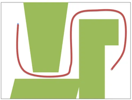
Figure 1.3: Workspace vs Configuration space: This planning situation requires the triangle to move translationally (no rotation) from the blue to the pink position. The left image contains the start and final configurations, while the right image maps it to its configuration space. The initial and final configurations can be represented as a point in C while the C−obstacles have been enlarged. Here, the F is the white area on the right image.

Using these definitions, we pose the basic motion planning as follows: Given a robot

r in workspace D and its initial and goal configurations, qinit and qgoal, respectively,

find a collision-free path τ such that τ(0) =qinit and τ(1) = qgoal, or report that such

a path does not exist.

1.1.2 Prior Approaches

A variety of approximations have been proposed and can usually be classified into a few

categories.

• Complete motion planning and cell decompositions: Many of the early

ap-proaches in motion planning compute an exact representation of the freespace, F.

(29)

report that no path exists. One of the more popular approaches for this is cell

decomposition planners [SS83,BLP85]. The idea of cell decomposition planners is

that the configuration space can be divided into regions of non-overlapping cells.

The size and type of cell is usually chosen such that a path exists between any

configurations within a cell and it can be determined whether or not the cell is

in F. After determining all of the “free” cells, a connectivity graph is generated

by using the adjacency relationships between cells. To solve a planning query, the

algorithm first identifies which cells contain the initial and goal configurations and

then performs a graph search through the connectivity graph between these cells.

The final path is extracted from the returned sequence of cells.

Other complete motion planning approaches, often also called criticality-based

al-gorithms, include computing the free space for a specific class of robots [LPW79,

Don84, Hal02] and exact roadmap methods [Can88a]. However, due to the

com-plexity of exact geometric queries for higher degree of freedom problems, there are

no known practical and efficient implementations of these complete approaches

[HH03]. Several hybrid planners which include cell decompositions have been

proposed as well, many of which are complete [VM05, ZKM07]. Others are

con-sidered resolution-complete and work by subdividing cells which are known to be

both “free” and contain a configuration space obstacles. Thus, for a sufficiently

small cell, they can report whether or not a path exists (See Fig. 1.4)

• Roadmaps: Roadmap approaches represent the connectivity ofF by a graph or

network of configurations and 1D collision-free curves connecting these

configura-tions. A roadmap is first constructed by sampling configurations inF (usually in

a randomized or otherwise prescribed manner) and then determining a local path

between these configurations. Given an initial and goal configuration, the planner

first determines how to connect each of these configurations to the roadmap. Then,

(30)

Figure 1.4: Cell decomposition: A vertical cell decomposition of the C is computed by extending the vertices of theC obstacles vertically to the environment boundary. A path is created by connecting the midpoints of adjacent cells.

of a planning query relies on the quality of the roadmap: how well it captures the

global connectivity of F and on how easily any configuration can be connected

to the roadmap. Recently, randomized approaches of roadmap generation

(Prob-abilistic Roadmap Methods [KSLO96], Rapidly-exploring Random Trees [LK00])

have been very successful at solving a wide range of complex problems and have

also been shown to be probabilistically-complete (See Fig. 1.5).

• Potential fields: These planners exploit the idea thatartificial potential functions

defined over the configuration space can be used as a heuristic to direct the path

search. Navigation potential functions are usually designed as a summation of an

attractive potential (or a sink) at the goal configuration, and repulsive potentials

(31)

Figure 1.5: Roadmap: A roadmap is created by randomly sampling the C. Each sample in F is then connected to the nearest neighbors on the roadmap. To find a path, the initial and goal configurations are connected to the roadmap. Then, the shortest path between the configurations is found and used as the path.

function for a robot with a configurationqt at timet may be:

Ur(t) = Uqgoal(t) +UO(t)

where

Uqgoal(t) =

1

2kp(qt −qgoal)

2

and

UO= X

oi∈O

1 2ko(

1

d(oi,qt)

− 1

ρ)

2

where Uqgoal is an attractive potential to the goal, and UO is the total potential

away from obstacles,kpis a potential gain for the goal,ko is a potential gain for the

obstacles, ρis a limit on the distance of the potential field influence, and d(oi,qt)

(32)

the potential field points toward lower potentials and thus away from obstacles

and toward the goal. In many cases, the potential function can be sampled locally

and does not need to be entirely precomputed. Similarly, this often lends itself to

real-time executions since the potential field at a point can usually be determined

very quickly [Kha86]. However, one well known drawback of this approach of

potential field motion planning is that the field could contain local minima. If

a robot moves into one of these regions, it effectively becomes stuck. A variety

of approaches help reduce the likelihood of this situation such as construction of

a potential field which does not contain any local minima [RK92] or by adding

Brownian motion or a random walk to the motion at each stage [BL91]. While the

exact approach is limited by the number of degrees of freedom in the problem, the

Brownian motion solution has been shown to work effectively for tens of degrees of

freedom. Due to the randomization, it is alsoprobabilistically-complete, or will find

a path if one exists given sufficient time. In general, probabilistic completeness

relaxes the requirement of path existence. (See Fig. 1.6).

While most work falls into the previously described categories, there are a few

ap-proaches which try to leverage the advantages and disadvantages of several of these

ideas. For instance, a coarsely defined roadmap does a good job of capturing the

gen-eral connectivity of an environment, while a potential field can help overcome difficulties

in navigating between the connected components. A roadmap could also be extracted

from a potential field by identifying the local minima checking if they can be connected

by a simple “link”.

The true success of any of these approaches is often measured by how large or complex

of a problem it can solve, and how quickly a solution can be found. While each of these

classes of planners or solvers have been extended to solve a wide variety of problems of

varying complexity, each has some inherent drawbacks. For instance, while the potential

(33)

Figure 1.6: Potential field: Since all obstacles here are given a repulsive or high potential value, this potential field path causes the robot to try to stay optimally far from obstacles as it navigates toward the goal.

is further away from obstacles. Furthermore, it is often perceived as being smoother

or more natural since the resulting path is smooth. The next two subsections discuss

additional topics: the range of problems which planning approaches can be used to solve

and the related complexity of these planning problems.

1.1.3 Extensions to basic planning

In many realistic or modern planning scenarios, the problem’s assumptions do not match

those of the basic motion planning problem. A wide variety of extensions to the basic

problem have been proposed. Since this work relates to several of them, we provide an

overview of the extensions related to our work here.

• Dynamic environments: In many scenarios, it is more realistic if the robot is

not the only entity moving in a scenario. For this extension, obstacles oi ∈ O

(34)

If the motion of a dynamic oi is known a priori, the configuration space can

augmented to include a temporal dimension t where oi(t) describes the state of

the obstacle at any point in time. On the other hand, if the motion of oi is not

predetermined or is influenced by interactions with the robot, then the planning

algorithms must be able to quickly adapt or replan as time proceeds to account

for changes in the environment. If the obstacles can be moved by the robot, the

planner could consider how an obstacle must move or how the moved obstacle

changes the connectivity when planning a path.

• Differential constraints: The basic planning problem requires finding a path

based only on the geometry of the robot. Other factors can influence or otherwise

restrict the way a robot can move. For instance, a wheeled robot typically has a

limited turning radius and moves based on the directions of the wheels. In other

cases limits on velocity and acceleration require second order constraints (over

time) to be maintained. These types of constraints are often generically classified

as differential constraints. A planner needs to consider a different

parameteri-zation of space which includes the robot’s state rather than just its geometric

configuration, which includes additional information such as a robot’s velocity or

acceleration. Planning algorithms must then consider the robots state-space S

and any state-space obstacles. Finally, other factors such as avoiding inevitable

collisions states, or states in which the momentum of the body will cause a

colli-sion in the future, should be considered. This category is often broken down into

three subcategories: nonholonomic planning, kinodynamic planning, and

trajec-tory planning. Briefly, nonholonomic planning is primarily mentioned in regards

to wheeled robots, and involves constraints which cannot be completely integrated.

Kindoynamic planning usually requires velocity and acceleration bounds to be

sat-isfied while also avoiding obstacles, thus the second order dynamics of the motion

(35)

determine a sequence of positions along with velocities (or velocity profiles) for a

robot that satisfy the dynamics constraints.

• Multiple agents: In many real and virtual world scenarios, a team of robots must

work together to solve a problem, or several agents will move in close proximity to

each other to individually reach their goals. For both of these, the basic problem

needs to be extended to include several robots. One view of this extension is

that it is very similar to unpredictable obstacles, each robot is an unpredictable

obstacle to every other robot. However, unlike obstacles, each agent or robot

can be controlled. In another view, groups of robots or the entire population of

robots can be treated much like a single robot in a “combined” or “aggregated”

configuration space. Then, motion for the multiple agents can be generated in a

similar manner to the standard planning approach.

• Deformable or non-rigid robots: With recent improvements in simulation

and robotics technology, it is no longer a requirement to have rigid agents or

robots. For instance, consider motion planning for a flexible fire hose or rubber

tube, a bendable needle, or any other soft-bodied or otherwise pliable object.

Also, consider a situation where a robot needs to move or adjust a deformable

object. Since any point on the surface can be moved or deformed relative to

any other point, the parameterization of the space is often much more difficult.

In practical implementations, the bodies are discretized as a set of volumes or

control points. For a higher resolution deformable body, this leads to a very large

number of control points and extremely large configuration spaces (and intractably

long planning times). Furthermore, planners for general deformable robots must

consider soft-body constraints such as volume and total or degree of deformation

(36)

1.1.4 Motion Planning Challenges

Advances in motion planning methods and algorithms have had a difficult time keeping

up with growth of complexity of many current systems or situations. For instance,

med-ical practitioners could make use of a deforming catheter-like robot to aid in performing

various procedures. Related simulations could also help as a teaching tool or for

preoper-ative planning. Hyper-redundant robots such as snake-like robots or self-reconfigurable

modules may contain hundreds or possibly thousands of links and joints. Fleets of

mo-bile robots sizing from the tens to hundreds are already used for managing warehouses.

Autonomous vehicles will need to know how to avoid and navigate among many other

moving obstacles. Virtual reality developers can populate their environments with many

agents each of which have their own goal, task, or behaviors. All of these examples are

very difficult to handle in the current state of motion planning algorithms.

The complete robot motion planning problem has been shown to be exponential in

number of DOFs of the robot [Rei79,Can88b]. As previously mentioned, many modern

and popular approaches employ randomization to quickly generate an approximate and

hopefully representative mapping of theC, and they also relax the completeness

require-ment in the process. These algorithms have enjoyed a great deal of success over the last

decade due to their ability to solve a wide variety of problems in higher dimensional, or

high DOF, configuration spaces in a more practical amount of time. Moreover, these

randomized algorithms are generally intuitive and relatively easy to implement.

As the complexity of the robot or its environment increases, motion planning becomes

more and more difficult. When considering problems with deformable robots, highly

articulated robots, or multiple, complex robots such as those previously mentioned,

the effectiveness of most motion planning algorithms rapidly deteriorates. By nature

of randomized algorithms, the motion itself may not be even be realistic. Most of

these approaches generate motion by linearly interpolating between states rather than

(37)

is not necessarily physically plausible, is not smooth, or may contain motion paths which

are un-intuitive. There are some approaches which plan in the “state” space of a robot,

sometimes referred to as “kinodynamic” planning [HKLR02]. However, since kinematic

and dynamic constraints increase the dimensionality of the space which needs to be

searched, they typically do not scale well to higher DOF planning scenarios.

Based on these considerations, we identify three important sources of complexity in

motion planning for realistic, and more generic, scenarios:

1. Agent complexity: The complexity is inherent to the robot itself or to its

ge-ometry. For instance, for a highly articulated robot with thousands of joints and

possibly many branches or kinematic loops, the C has an extremely high

dimen-sionality. As mentioned in Sec. 1.1.3, for a completely deformable robot theC may be intractably large. In both cases, the complexity of the robot is typically too

great for standard planning approaches. Finally, to ensure smooth and realistic

motions, dynamics and kinematics for these robots should be considered. Since

each parameter in the “state” space adds additional DOFs to the problem, these

constraints can also greatly increase the overall problem complexity.

2. Numerous agents: Many real world and virtual planning situations include

multiple moving bodies, or multiple agents. A complete, centralized approach to

this situation treats the DOFs of all the robots as a single robot, i.e. a single

configuration describes the complete position and orientation of all robots and

their sub-parts. Under this formulation, the problem is identical to the

single-robot planning problem and can be handled as such (via any of the approaches

mentioned earlier). Since the number of DOFs grows linearly with the number of

robots, the inherent complexity of the planning problem becomes intractable with

just a few robots. Decentralized approaches treat each robot individually; they

plan for each robot individually and then perform a coordination planning step to

(38)

The latter solution is usually faster, but gives up the completeness property of a

centralized algorithm and in practice has been shown to have a much lower success

rate [SI06].

3. Dynamic environments: Finally, in many cases, there are other obstacles or

items which are moving or are otherwise changing during the execution of the

motion. These dynamic events and environments add complexity to the planning

situation itself, and present additional challenges. In cases where the motion of

obstacles is unpredictable, it adds a real-time constraint. The robot has a finite

amount of time to decide how to avoid or adapt to a changing environment. In

many cases, this requires the robot to quickly re-plan or otherwise adapt its current

plan. Since planning is already a complex task, this poses a large challenge for even

moderately complex environments. When the obstacle motion is known a priori,

this adds a temporal dimension toC which makes planning more computationally

expensive due to the larger search space.

In many real and virtual world situations, many of these constraints may exist even

in a single situation or scenario. For instance, a city scene may include navigating

agents which must also avoid moving vehicles. While algorithms do exist which can

appropriately handle for each of them individually, the ability to do this successfully

and in a reasonable amount of time diminishes as the problems become more complex.

Even for moderately “realistic” problems, most modern motion planning algorithms

tend to take a long time or do not respond in a practical amount of time.

1.2 Constrained Simulation

Motion planning has enjoyed a great deal of success in providing specific, goal-oriented

(39)

high. On the other hand physics simulators, systems or software which can adequately

model physics and physical interactions, have seen successes in handling large numbers of

objects in a general, unified manner, in a physically realistic manner, and in a relatively

faster amount of time.

With regards to robots, agents, and environments, many simulation environments

provide a uniform set of “motion equations,” or predefined rules or laws which dictate the

motion of a body, based on well established laws such as those of classical dynamics. This

permits any object in a scene to behave in a physically-plausible way: they accelerate,

torque, recognize collisions, and respond to collisions much like one would expect it

to respond. Constrained simulation augments standard simulation environments by

restricting or otherwise influencing the way an object can move. For example, consider

a hinged joint with two pieces, such as one that allows a door to open and close. One

solution to generate motion in this situation is for all the interactions between both

parts of the joint to be modeled. Since they are always in contact, there would be an

infinite number or extremely high number of contacts each of which would need to be

resolved. Instead, since we know by design that both parts of the hinge will always be in

contact, we can ignore these complex interactions and instead constrain the motion of

the two pieces to behave in this manner, like an articulated body. This greatly reduces

the computational complexity while still allowing for realistic simulations.

In this sense, constrained dynamics allows a body to follow and obey the established

motion laws and equations while also requiring it to obey the defined constraints and

restrictions. In a way, it gives more “control” over a simulation but still benefits from

the generalized simulation framework. This aspect of constrained simulation makes it a

good fit to aid in motion planning.

In this section we give a brief overview of a general simulation framework, describing

the primary tasks which a simulator needs to implement. A more complete treatment

(40)

limitations in using constrained dynamics specifically for the task of motion planning.

1.2.1 Physically-based simulation

Most physics and dynamics simulators share common elements, regardless of what they

are attempting to simulate. This includes a set of motion equations which dictates

how the body moves given a set of external (and sometimes internal) forces, a collision

or interference query system which finds the set of overlapping geometry, a collision

response system which determines how to respond or react to collisions, and finally a

numerical solver which is used to evolve the state of the environment in time.

For example, consider a simple particle: a point in space with a mass. Its motion can

be most easily described via the Newton-Euler laws of motion. Collisions are detected

when the particle crosses any surface or plane in the environment, and a response can be

calculated by simply reflecting its currently velocity (and eliminating any acceleration in

the direction of the surface with which it collided). Finally, Euler’s numerical integration,

or any other numerical integration technique, can be used to solve the motion equations

and to update the state of the particle.

While this is a simple example, nearly all physical simulators have a similar

frame-work. The motion of rigid, articulated, and even deformable bodies can be described by

some equations. A wide variety of collision detection and response methods have been

studied for each of these classes of bodies, and a wide range of methods are available to

update the state. Regardless of the choice of components, the end result is a simulator

which reflects whatever behavior is encoded into the system.

1.2.2 Constraint-driven simulation

Standard physics simulators have been successful used in numerous applications, mainly

when the emphasis is on the evolution of the motion or the trajectory of objects in a

(41)

constraint-driven or constrained simulation is that we want to be able to do more than

apply external forces, we want to be able to actually restrict the way the bodies are

allowed to move in a scene or environment. This is an important concept in general,

as it paves the way for more compelling and efficient simulations. Constraints allow us

to connect two bodies via hinge, require that certain bodies stay a fixed distance apart,

ensure that no pair of bodies are overlapping or interesting, and many more.

In the scope of this work, constraints generally fall into two different categories.

Hard constraints are firm restrictions on the motion or state and must be enforced at

all times whereas soft constraints are used to influence the motion or behavior at a

given state, but are not required to be maintained at all times. Thus, hard constraints

directly remove or changes properties of the body or its forces whereas soft constraints

act alongside (or in opposition to) external forces. When combined, these constraints

greatly enhance the capabilities of a simulation.

For example, consider a “point-distance” constraint between a pair of pointsxandy.

Thishardconstraint could be useful for fixing two points on a robot or ensuring that the

robot stays a fixed distance from some other object. Mathematically, this constraint can

be defined asCdist(x,y) =||x−y|| −d for some specified distance d. During execution,

if Cdist 6= 0, then let δd be the difference between d and the actual distance. We can

move each body a distance of δd

2 toward each other to enforce the constraint or apply a

force that would cause the same change in position.

Alternatively, consider a “goal attraction” soft constraint. This constraint can be

defined such that it will only be satisfied once the robot, or whatever part of the robot

the constraint is defined on, reaches its goal. A penalty force for this constraint would

point directly toward the goal or along a path, and could be applied to the entire robot

or to whatever part of the robot needs to reach the goal.

Many more details and specific examples of hard and soft constraints will be

(42)

1.2.3 Simulation loop

To this point, we have discussed the main concepts for a constrained simulation. The

simulation loop ties these components algorithmically in order to generate

physically-plausible motion.

Note that we have not yet put all the pieces together into a single, unified system.

Many related works describes a simulation core or a simulation loop to achieve this. The

following are the general steps in a single step of a simulation core:

1. Clear the force accumulators: Each body or its components maintains a total

of all forces on it. At the beginning of each step, we clear the forces from the

previous step.

2. Detect collisions: Loop over all bodies and determine any contacts or collisions

in the scene and prepare them to be resolved.

3. Compute external forces: Loop over all external forces, including contact or

collision resolution forces, and add them to the force accumulators.

4. Compute constraint forces: At this point, each body or component knows the

total force acting upon it (its in force accumulator). To process the constraints,

first add any soft constraints to the accumulators. Finally, compute and apply the

hard constraint forces.

5. Compute derivatives: Gather derivatives as needed to prepare to update the

system.

6. Integrate and update the state of the simulation: Use a numerical

(43)

1.2.4 Constrained simulation challenges

Constrained simulation is a powerful framework for generating motion of many bodies.

A simple set of rules and constraints can be defined which will handle an extremely wide

variety of situations. As such, it has become an extremely popular tool in interactive

computer graphics, animation, and even in robotics. However, there are several

chal-lenges and complications inherent to physics simulation with respect to the goal of this

work.

• Computational bottlenecks: A wide variety of geometric and numerical methods

are used to determine the state of the bodies in the environment, interactions

between the bodies, their derivatives, and finally to advance the simulation in

time via numerical integration. Since these steps must be performed at every step,

the performance of a simulation dependent on the complexity of these methods.

Algorithms for the simulation core must be chosen to not only be accurate, but

also efficient, in a wide range of applications.

• Motion per step: Even if the simulation core is efficient, the overall simulation can

still take a great deal of time. For instance, if our time step is extremely small

or if the simulation’s goals require a the body to travel a great distance (relative

to the maximum amount it can travel per iteration) then the overall simulation

can still take a great deal of time. Thus, simulation core algorithms should try to

allow for large steps either in time or motion available.

• Stability: A well known drawback of several numerical integration techniques is

their instability. In particular, many integration methods suffer fromstiff systems

and when the time step is too large. Compelling simulations need to be aware of

the complete range of interactions possible in order to try to avoid this state. While

(44)

simulation parameters can help overcome some of these drawbacks, these can also

significantly impact performance.

• Constraints: In general, there is a standard set of constraints like non-penetration

and collision response we can be included in any simulation. However, many

sim-ulations, such as hinges or joints as mentioned earlier, require specific additional

constraints. Thus, to some degree, every problem must be evaluated for which

con-straints are necessary. Furthermore, many of these concon-straints include constants

which must be tuned depending on the range of interactions and other dynamics

of the simulation.

• Accuracy and error: To help improve performance, many portions of a

simula-tion core are often approximated. The time-integrasimula-tion methods and computasimula-tion

of derivatives are examples of methods that are often approximated or that can

include some additional error. Given the simulation loop, these errors can

accu-mulate over the duration of a simulation. Thus, components of the simulation

core must be precise enough to either correct for errors or keep them at a

reason-ably small level, but fast enough to be able to solve problems within a reasonable

amount of time.

While these topics each present challenges for simulation, they are common across

most simulation environments. Due to the popularity of simulation or simulation-related

techniques, a great deal of attention has been given to these topics to help alleviate or

reduce the impact of them. Nonetheless, they are important considerations in using

simulation as part of general motion planning.

1.3 Goals

In the previous sections, we describe two variations on ways to control motion of bodies

Physically-based sampling for motion planning