A comparison of performance of K-complex classification
methods using feature selection
Elena Hernández-Pereira, Veronica Bolón-Canedo, Noelia Sánchez-Maroño, Diego Álvarez-Estévez,
Vicente Moret-Bonillo, Amparo Alonso-Betanzos
Department of Computer Science, Faculty of Informatics, University of A Coruña, Campus de Elviña s/n, 15071 A Coruña, Spain
Keywords: Feature selection Machine learning, K-complex classification.
A b s t r a c t
:
The main objective of this work is to obtain a method that achieves the best accuracy results with a low false positive rate in the classification of K-complexes, a kind of transient waveform found in the Electroencephalogram. With this in mind, the capabilities of several machine learning techniques were tried. The inputs for the models were a set of features based on amplitude and duration measurements obtained from waveforms to be classified. Among all the classifiers tested, the Support Vector Machine obtained the best results with an accuracy of 88.69%. Finally, to enhance the generalization capabilities of the classifiers, while at the same time discarding the existing irrelevant features, feature selection methods were employed. After this process, the classification performance was significantly improved. The best result was obtained applying a correlation-based filter, achieving a 91.40% of accuracy using only 36% of the total input features.
1. Introduction
Sleep staging classification is one of the most important tasks within the context of sleep studies. Over the last few decades the gold standard for the characterization of patients’ sleep macrostructure has been based on the set of rules proposed by Rechtschaffen and Kales (R&K) [37], which assigns labels to time intervals representing different states of sleep: Wakefulness (W), stages 1–4, and Rapid Eye Movement (REM). This method has been recently modified by the American Academy of Sleep Medicine (AASM) [23] which reduced the four non-REM stages into only three stages: stage 1, stage 2 and stage 3 (this last being the union of what were previously stages 3 and 4). To help in sleep stage characterization, a micro structural analysis is necessary. Transient events such as micro arousals, sleep spindles, K-complexes and other patterns need to be analyzed [23].
According to the current AASM definition [23], K-complex is a “well-delineated negative sharp wave immediately followed by a positive component standing out from the background Electroencephalogram (EEG), with total duration ≥ 0.5 s, usually maximal in amplitude when recorded using frontal derivations”. Some works have also imposed a maximum duration generally comprised between 1 and 3 s
[8,26,27,38,39]. K-complexes are one of the key features that contributes to sleep stages assessment, specifically is one of the hallmarks of stage 2. Unfortunately, their visual identification is very time-consuming (there are typically 1–3 K-complexes per minute in stage 2 of young adults [28]) and rather dependent on the knowledge and experience of the clinician, since it cannot be performed on a regular basis. Hence, poor agreements among experts are reported in the literature
[8,40]. This explains why automatic identification of complexes is of great interest. The main difficulty of the automated K-complex identification problem has been the lack of specific characterization of the wave and its similarity to other EEG waves such as delta or vertex waves. In spite of this difficulty, this task has been the purpose of several published efforts that will be analyzed in more detail in the next section.
Based on shape analysis, one of the most relevant works in the K-complex detection so far has been that of Bankman et al.
[4], where a feature-based detection approach is presented. However, analysis of the relevance of the different features has not been fully carried out, so our fundamental hypothesis is that classification of K-complexes based on shape analysis can be improved by the application of feature selection methods. This paper deals with the extraction and classification of isolated waveforms. The capabilities of several machine learning techniques were tried for this classification task where the inputs for the classifiers were the features described in Bankman’s work, based on amplitude and duration measurements. To enhance the generalization capabilities of the classifiers, while discarding the existing irrelevant features, feature selection methods were employed. Feature selection is arguably the most popular dimensionality reduction technique, whose goal is to obtain a subset of features that properly describes the given problem attempting to improve the classification performance and generalization capacity[16]. Moreover, there are other benefits associated with a smaller number of features: a reduced measurement cost and hopefully a better understanding of the domain. These facts have been demonstrated in earlier work by the authors of this paper for the identification of EEG arousals[3]. Given the properties mentioned above, feature selection is a broadly used technique in the machine learning field[7,43,49]. In order to investigate the previous hypothesis, the goal of this research is therefore to propose a reduction in the number of necessary features whilst improving the K-complex classification accuracy.
The paper is structured as follows:Section 2presents different methods available to identify K-complex patterns,Section 3
proposes the research methodology,Section 4describes the materials and methods used in the research,Section 5presents the results obtained and, finally, discussion and conclusions are presented inSection 6.
2. Background
Several attempts for K-complex automatic identification have been found in the literature : some of them deal with the K-complex wave detection[8,11,12,26,27,41,42,44]and work with the complete night recording while others deal with the clas-sification problem[4,24,25,34,35,38,47]using EEG segments of fixed length to determine if they are K-complexes or not.
The firsts attempts trying to characterize the K-complex waves, involved the design of an electronic detection system capable of operating in real time, although the accuracy of the detection system is argumentative[8]. Later, Jansen et al. describe in[25]
a knowledge-based approach to automated sleep EEG analysis. The system is tested on the detection of K-complexes and sleep spindles and its performance indicates that the approach followed is feasible but the data set used is not meaningful. Another explorative study[24]investigates the performance of artificial neural networks (ANN) for the detection of K-complexes using the raw and filtered digitized data but this approximation leads to poor results. A detector of vertex waves and K-complexes has been proposed by Da Rosa et al., which models neuronal feedback loops and detects the transient events through a maximum-likelihood estimator[39]. In real sleep signals, the number of K-complexes detections in which automatic and visual scoring agreed reaches a level of 94% with a false positive rate of 13%.
In 1992, Bankman et al.[4]present a feature-based detection approach using ANNs that provides good agreement with visual K-complex recognition. A sensitivity of 90% is obtained with about 8% false positives (FPs). The information contained in the features provides significantly better results than the classification based on raw data, as the work states.
Later, Jansen presents a study aimed to improve Bankman and his own results[25], using simulated and real EEG data involv-ing two basic ANNs architectures[26]. These ANNs received normalized magnitude and phase values, obtained through Fourier transformation, as input. Nevertheless, the results achieved over real data are disappointing with poor classification rates for both network approaches. Even better results were obtained using the knowledge-based approach with the same data. Tang and Ishii present in[44]a method for recognizing the K-complex waveform based on Discrete Wavelet Transform parameters instead of amplitude and frequency in time-domain analysis. The method is tested on records of EEG containing auditory evoked K-complexes, obtaining 87% and 10% true and false positive rates, respectively. However, they considered the K-complex to be overridden by a sleep spindle but it can also occur isolated or even accompanied by alpha events (K-alpha) or embedded with delta waves[19]. In[42], the authors use a combined method of the one suggested by Bankman[4]and an ANN classifier as proposed by Jansen[24]. The features used as inputs to the classifier are a subset of those defined by Bankman with the goal of emulating visual recognition as closely as possible. Unfortunately, the authors do not provide numerical results.
Richard and Lengelle propose a detection structure which can be interpreted as joint time and time-frequency domains
[38]. Nevertheless, this structure does not deal with the detection of complexes but rather with the classification among K-complexes and delta waves. The performance reported in the K-K-complexes classification task is 90% true positive rate and 9.2% false positive rate, slightly worse than Bankman’s[4]. Kam et al. develop a novel algorithm based on Continuous Density Hidden Markov Model for K-complexes detection[27]. The approach is evaluated in two manners: first, using segments of K-complexes (classification problem) where it achieves a 7% error rate; and, second, using a whole night record (detection problem) where the performance is within the variance of the human scorers which achieve an average of 85.3% true positive rate.
In[11]a method based on feature extraction and likelihood thresholds is presented. The detection performance is evaluated on the basis of two human scorings performed independently. True positive rates of 61.72% and 60.94% are respectively obtained with scorer 1 and 2. Moloney et al.[34]develop a procedure based on nonsmooth optimization and classification methods. A combination of Radial Basis Function and Extended cutting angle method with a Multilayer Perceptron produced the best
3
Fig. 1. The K-complex classification methodology.
classification results. Lately, the attempts for K-complexes detection are in terms of comparing matched filter and ANN methods
[41]. The sensitivity obtained for the ANN is higher (96.06%) than the one obtained for the matched filter (86.47%). The inputs for the ANN are similar to Bankman’s features. Erdamar, Duman and Yetkin[12]proposed an algorithm for automatic detection of K-complex using amplitude and duration properties of the waveform. This algorithm is based on wavelet and teager energy operator combined to obtain a robust decision. The results obtained were evaluated with the ROC analysis and proved up to 91% success in detecting K-complex. In[47]a new feature extraction method is proposed. This method transforms visual features of the K-complex wave into mathematical representation and classifies it using a hybrid-synergic machine learning method. Their results indicate that the proposed model is at least as good as human experts in K-complex detection. Recently, in[35]
feature extraction with a Generalized Radial Basis Function Extreme Learning Machine algorithm is applied to obtain K-complex waves from EEG signals. In addition, they use feature selection to reduce the input space and improve their performance results. However, they only tested a feature selection method; it is based on a Sequential Forward Selection strategy and the Mahalanobis distance between classes as evaluation function. A fair comparative study is not possible due to differences in both datasets and evaluation methods.
To the best knowledge of the authors of this paper there is only an attempt[35]in the literature to take advantage of fea-ture selection methods in order to improve the classification performance, generalization capacity or simplicity of the induced model, in this specific field of application. Therefore, in this work several feature selection models are evaluated to confirm the aforementioned advantages.
3. Research methodology
The main objective of this work is to obtain a method that achieves the best accuracy results with a low FP rate in the K-complexes classification task. Over the EEG signal of a set of sleep recordings, and after applying a band filter, a set of isolated waveforms were obtained. Using these patterns, two approaches were tested. The first uses the set of 14 Bankman’s features
[4]and over a set of classifiers, chooses the best one in terms of accuracy. The second approach uses feature selection over the 14 features previously mentioned to check whether irrelevant features exist and, again, to choose the best classifier in terms of accuracy with the selected features. The goal of this second approach is to achieve comparable or better results than the first one, and also check the existence of possible redundant or irrelevant features that could be discarded so as to obtain a simpler final model. An outline of the proposed methodology is shown inFig. 1.
0 50 100 150 200 250 300 350 400 450 500 -40 -30 -20 -10 0 10 20 30 40 0 50 100 150 200 250 300 350 400 450 500 -80 -60 -40 -20 0 20 40 60 80
(a) Positive (b) Negative
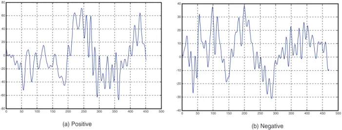
Fig. 2. Positive and negative K-complex examples.
Table 1
The features of the K-complex defined by Bankman.
Feature Formula Explanation
f1 xmax−xend Peak-to-peak amplitude
f2 xmax−xstart Amplitude of the sharp positive wave
f3 xstart−xend Difference between the start point and the minimum of the negative wave
f4 tend−tstart Trough-to-trough duration
f5 tmid1−tbase1 Duration of the sharp wave
f6 tmin−tmax Duration of the falling slope
f7 tbase2−tbase1 Duration at the baseline
f8 f5/f7 Ratio of the positive wave’s width to the baseline wave’s width
f9 (tlevel2−tlevel1)/(tbase2−tmid2) Sharp of the negative wave
f10 (tmid2−tmid1)/(tmin−tmax) Continuity of the falling side
f11 f1/f4 Aspect ratio of the wave (global sharpness)
f12 (xmax−xstart)/(tmax−tstart) Slope of the rise
f13 f2/f1 Ratio of the positive wave’s to the peak-to-peak amplitudes
f14 NttminmaxcrossBaseline Number of the times the baseline is crossed intmaxtotmin
3.1. Data processing
The initial step of the proposed methodology is the processing of the available EEG signals. It is widely known that the EEG signal is very sensitive to noise, which may hinder the identification of the features as proposed by Bankman[4]. In order to overcome this problem, the raw data was digitally filtered using two different criteria. In the first one we tried to get rid of, as much as possible, all of the frequency components outside the characteristics band of the K-complexes. In this respect we used a band-pass filter in the 0.5–2.3 Hz frequency band, with the resulting data identified asDataf. And, in the second one, we investigated a less conservative approach in which only the very high frequency components were filtered out by means of a low-pass filter with cut-off at 18 Hz. The resulting data is referred to asDataf2.
The next step in the methodology is to obtain the isolated waveforms. The positive examples were identified by the medical expert and in order to achieve a balanced data set, the same number of negative examples were selected from the whole set of recordings. To get these negative examples, the Bankman features were calculated for each recording over signal segments of three seconds duration, due to the K-complex maximum duration[11]. Then, the signal segments with an appropriate value for the first Bankman feature, the peak-to-peak amplitude, were selected and the segments corresponding to positive examples were discarded.
Fig. 2shows an example of a K-complex pattern identified by the medical expert,Fig. 2(a), and an example of background EEG waveform,Fig. 2(b), i.e., a negative example as previously described. Due to the highly stochastic nature of the EEG, a K-complex can have a large variety of shapes and it is not always distinctly different from the background EEG, as can be seen in the figure. The positive example is a arguable case as it is superimposed with varying levels of higher frequency EEG and its morphology is somewhat altered. Nevertheless it is a K-complex confirmed by the medical expert. The negative example is not a K-complex due to subtle differences presented in some features, such as the sharp of the negative wave and the slope of the rise (f9andf12 inTable 1respectively).
5
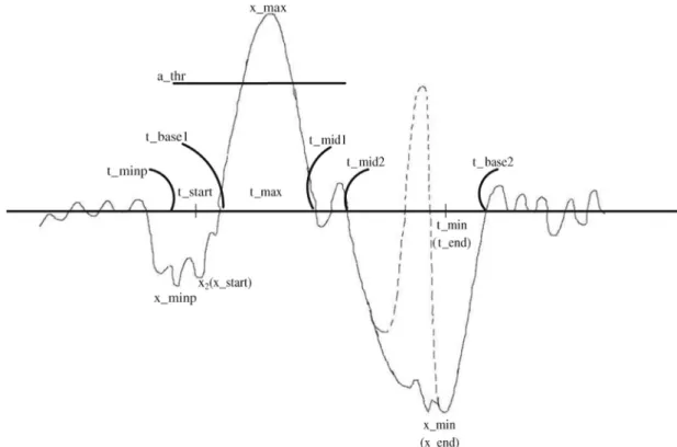
Fig. 3.A schematic K-complex with amplitude and time labels.
3.2. Feature extraction
As we have pointed out, the features used are those defined in[4], based on several amplitude and duration measurements taken on significant points of the K-complex waveform.Fig. 3shows a schematic K-complex in which the timing and amplitude labels of the significant points are marked.
Table 1describes the whole set of features.
3.3. Feature selection
Feature selection is a dimensionality reduction technique which consists of detecting the relevant features and discarding the irrelevant ones[16]. This technique has several advantages, such as:
• Improving the performance of machine learning algorithms.
• Data understanding, gaining knowledge about the process and helping to visualize it.
• Data reduction, limiting storage requirements and helping in reducing costs.
• Simplicity, possibility of using simpler models and gaining speed.
Feature selection methods can be divided into wrappers, filters and embedded methods. While wrapper models involve optimizing a predictor as part of the selection process, filter models rely on the general characteristics of the training data to select features with independence of any predictor. The embedded methods generally use machine learning models for classification, and then an optimal subset or ranking of features is built by the classifier algorithm. On the other hand, wrappers and embedded methods tend to obtain better performances but at the expense of being very time consuming and having the risk of overfitting when the sample size is small. On the other hand, filters are faster and, therefore, more suitable for large data sets. They are also easier to implement and scale up better than wrapper and embedded methods. For all these reasons, filters will be the focus of this work.
Three feature selection methods were chosen for this study, among those available throughout the literature[6], namely Correlation-based Feature Selection (CFS), Consistency-based filter and INTERACT, with the aim of employing filters that use different metrics to select the final features. CFS is one of the most well-known and most frequently used filters, INTERACT is based on the interaction between features and, finally, Consistency-based is based on the consistency in the class values. A detailed explanation of each filter method is given in the following sections.
3.3.1. Correlation-based feature selection, CFS
Correlation based feature selection is a simple filter algorithm that ranks feature subsets according to a correlation-based heuristic evaluation function[17]. The bias of the evaluation function is toward subsets that contain features that are highly correlated with the class and uncorrelated with each other. Irrelevant features should be ignored because they will have low correlation with the class. Redundant features should be screened out as they will be highly correlated with one or more of the remaining features. The acceptance of a feature depends on the extent to which it predicts classes in areas of the instance space not already predicted by other features. CFS’s feature subset evaluation function is:
MS=
krc f
k+k
(
k−1)
rf f, (1)
whereMSis the heuristic ‘merit’ of a feature subset S containingkfeatures,rc f is the mean feature-class correlation (f∈S) and
rf f is the average feature–feature intercorrelation. The numerator of this equation provides an indication of how predictive of the class a set of features is; and the denominator of how much redundancy there is among the features.
The application of this algorithm consists of two steps. First, the numeric features are discretized and then, a measure known asSymmetrical Uncertainty, SU[36], is employed. SU is defined as the ratio between the information gain (I) and the entropy (H) of two features,XandY:
SU
(
X,Y)
=2 I(
X;Y)
H
(
X)
+H(
Y)
, (2)where:
• The entropy (H) quantifies the uncertainty present in the distribution of a featureX, randomly chosen, and it is defined as
H
(
X)
= −x∈X
p
(
x)
logp(
x)
,where the lower casexdenotes a possible value that the variableXcan adopt.
• The Information Gain (I) is defined as
I
(
X;Y)
=H(
Y)
+H(
X)
−H(
X|
Y)
,beingH(X) the entropy of featureXandH(X|Y) the entropy of featureXonce the values taken by another featureYare known, computed as:
H
(
X|
Y)
= −y∈Y
p
(
y)
x∈X
p
(
x|
y)
logp(
x|
y)
.The value of IG denotes the relevance of a given feature with respect to others. Thus, in the case thatIG(X,Y)>IG(Z,Y) it is demonstrated that featureYis more correlated with featureXthan with featureZ.
Returning to the CFS algorithm, the SU measure (Eq. (2)) is used to estimate the degree of association between two different features and, then, obtaining different subsets of features. In the second step of the algorithm, we useMS(Eq. (1)) to select the optimal subset of features.
3.3.2. Consistency-based filter
The consistency-based filter[10]evaluates the worth of a subset of features by the level of consistency in the class values when the training instances are projected onto the subset of attributes. The algorithm generates a random subset S from the number of features in every round. If the number of features of S is less than the current best, the data with the features prescribed in S is checked against the inconsistency criterion. If its inconsistency rate is below a pre-specified one, S becomes the new current best.
The inconsistency criterion, which is the key to the success of this algorithm, specifies to what extent the dimensionally reduced data can be accepted. If the inconsistency rate of the data described by the selected features is smaller than a pre-specified rate, it means that the dimensionally reduced data is acceptable.
The inconsistency rate is calculated as follows:
(a) Two patterns are considered inconsistent if they match all but their class labels. For example, an inconsistency is caused by two instances (0 1, 1) and (0 1, 0), in which the two features take the same values for these two samples, while the class attribute varies.
(b) The inconsistency count for a pattern is the number of times it appears in the data minus the largest number among different class labels. For example, let us assume there arenmatching patterns, among whichc1patterns belong to label1;
c2to label2andc3to label3wherec1+c2+c3=n. Ifc3is the largest among the three, the inconsistency count is
(
n−c3)
. (c) The inconsistency rate is the sum of all the inconsistency counts for all possible patterns of a feature subset divided by the7
3.3.3. INTERACT
The INTERACT algorithm[50]is a method based on symmetrical uncertainty (SU)[36], defined inEq. (2), that introduces the detection of interaction between features.
The motivation behind the development of this algorithm is based on the idea that, in theory, a feature not very correlated with the class label might be deemed as irrelevant. However, if it is combined with other features, it might be highly correlated with the class label, becoming an important feature for the prediction task. Dealing with the possible interaction between all the features is practically unfeasible, and that is why algorithms previous to INTERACT seldom tackle this problem and they usually assumed independence between features.
The authors of INTERACT consider that the interaction between features can be managed with a thorough design of the evaluation measure (consistency contribution) and a backward search strategy.
The main measure employed by this algorithm, besides SU (Eq. (2)), is the consistency contribution (c-contribution). C-contribution of a feature is an indicator about how significantly the elimination of that feature will affect consistency. The algorithm consists of two major parts. In the first part, the features are ranked in descending order based on their SU values. In the second part, features are evaluated one by one starting from the end of the ranked feature list. If the c-contribution of a feature is less than an established threshold, the feature is removed, otherwise it is selected. The authors stated in[50]that INTERACT can thus handle feature interaction, and efficiently selects relevant features.
3.4. Classification
In this section, we provide an overview of the methods used in the research for K-complex classification (seeFig. 1). Several approaches were considered, three lineal models —a one-layer feedforward neural network, a logistic regression and a proximal support vector machine—, and two non linear ones —a multilayer feedforward neural network and a support vector machine—.
• One-layer feedforward neural network
The one-layer feedforward neural network (FNN) is a single-layer FNN without hidden layers. This is a linear classification system that was trained using the supervised learning method proposed in[9]. The contribution of this learning method is that it is based on the use of an alternative cost function that measures the errorsbeforethe nonlinear activation functions instead ofafterthem, as is normally the case. An important consequence of this formulation is that the solution can be obtained directly using a system of linear equations due to the fact that the new cost function is convex[13]. So, the method avoids local minima, and a very good approximation to the global minimum of the error function is obtained.
• Logistic regression
Logistic regression is part of a category of statistical models called generalized linear models. The goal of logistic regression is to correctly predict the category of outcome for individual cases using the most parsimonious model. To accomplish this goal, a model is created that includes all predictor variables that are useful in predicting the response variable. Logistic re-gression does not assume a linear relationship between the dependent (outputs) and independent variables (inputs), finds a “best fitting” equation using a maximum likelihood method, which maximizes the probability of getting the observed results given the fitted regression coefficients[32].
• Multilayer Feedforward Neural Network
The multilayer feedforward neural network is one of the most commonly used neural network classification algorithms
[5]. The architecture used for the classifier consisted of a two layer feed-forward neural network: one hidden and one output layer. It has been demonstrated that, with an appropriate number of hidden neurons, one hidden layer is enough to model any continuous function[21]. The optimal number of hidden neurons for this problem was empirically obtained.
• Support Vector Machine, SVM
A Support Vector Machine is a supervised classification technique that works by nonlinearly projecting the training data in the input space to a feature space of higher (infinite) dimension by the use of a kernel function. This results in a lin-early separable data set by a linear classifier. In many instances, classification in high dimension feature spaces results in overfitting in the input space; however, in SVMs, overfitting is controlled through the principle of structural risk mini-mization[46]. The empirical risk of misclassification is minimized by maximizing the margin between the data points and the decision boundary[30].
• Proximal Support Vector Machine, pSVM
The proximal Support Vector Machine[14]is a method that classifies points assigning them to the closest of two parallel planes (in input or feature space) that are pushed as far apart as possible. The difference with a SVM is that this one classi-fies points by assigning them to one of two disjoint half-spaces. The pSVM leads to an extremely fast and simple algorithm by generating a linear or nonlinear classifier that merely requires the solution of a single system of linear equations.
3.5. Performance measures
After the classifiers were trained, the performance of the system is evaluated in terms of different measures of relevance to the problem in question. The definitions of the performance measures are provided as follows:
• The classification accuracy is computed as the percentage of correctly classified instances on a data set.
• The sensitivity (or true positive rate) is the proportion of K-complexes which are correctly identified as such.
In the context of K-complex classification, it is preferable to miss a K-complex rather than to false identify it[4]. Therefore, it is interesting to minimize the false positives while retaining a satisfactory level of sensitivity.
3.6. Multiple-criteria decision-making, MCDM
Classification algorithms are normally evaluated in terms of multiple criteria which can be handled by a single evaluation model using Multiple-Criteria Decision-Making[48]. This model is focused on addressing the aforementioned issue. MCDM methods evaluate classifiers from different aspects and produce rankings of classifiers[15]. Among many MCDM methods that have been developed up to now, Technique for Order of Preference by Similarity to Ideal Solution (TOPSIS)[22]is a well-known method that will be used. TOPSIS finds the best algorithms by minimizing the distance to the ideal solution whilst maximizing the distance to the anti-ideal one.
4. Materials and methods
The aim of this work is to present a methodology to improve previous results on K-complex classification presented in Bankman et al. study[4]. The materials and methods used in this work are described in this section.
4.1. Datasets
In the experiments made, 32 different recordings scored at the Brain Research Center of the Medical University of Vienna were used. The EEG signals of these recordings were sampled with a frequency of 200 Hz and later analyzed by a medical expert who detected a total of 111 K-complexes.
According to the methodology shown inSection 3.1, two approaches for filtering the data were applied, resulting in two banks of data namedDatafandDataf2. Then, and in order to achieve a balanced set, the same number of negative examples were selected from the whole set of recordings. In this manner, bothDatafandDataf2data sets have 222 samples.
4.2. Experimental procedure
The experimental procedure is detailed as follows: 1. Extract the initial set of features to be used as inputs.
2. Apply the three feature selection methods (CFS, Consistency-based filter and INTERACT) presented inSection 3.3to provide the subset of features than describe properly the given problem.
3. For each nonlinear classifier, establish its architecture/parameters.
(a) For FNNs, set the number of hidden units by training independently each of the FNNs. In order to choose this num-ber, the results stated by Hecht-Nielsen[20]were used. These results establish that a FNN should never possess a number of hidden units more than twice plus one the number of its input units (i). Therefore, several FNN topolo-gies were trained using from 2 to 2 times i + 1. Then, for the multilayer model set the number of output units (1 vs. 2). Among these models, we try a one hidden layer architecture and a two hidden layer architecture. Logistic transfer functions were used for each neuron in both the hidden and the output layers. The learning algorithm used was the conjugate gradient[33]with the mean squared error cost function. A maximum number of 3000 epochs were performed on the training set.
(b) For the SVM, set the kernel function. We try a linear, polynomial of degree 2, and Gaussian (choosing different sigma values: 1, 100, 1000, 10,000) kernel functions. The cost parameter value was set to values in the range [100,∞]. 4. Take the whole data set and apply a 10-fold cross validation in order to better estimate the true error rate of each model. 5. Obtain the accuracy measures, and a decision threshold for the output of each model and select the best one. For the
resulting model obtain false positive rate and sensitivity measures.
6. Apply the TOPSIS method to the performance measures previously obtained.
The experiments performed in this work were executed using the software tools Matlab and Weka, described as follows:
• Matlab[31]is a numerical computing environment, well known and widely used by scientists and researchers. It was de-veloped by MathWorks in 1984 and its name comes fromMatrix Laboratory. Matlab allows matrix manipulations, plotting of functions and data, implementation of algorithms, creation of user interfaces, and interfacing with programs written in other languages, including C, C++, Java, and Fortran.
• Weka (Waikato Environment for Knowledge Analysis)[18]is a collection of machine learning algorithms for data mining tasks. The algorithms can either be applied directly to a data set or called from your own Java code. Weka contains tools for data pre-processing, classification, regression, clustering, association rules, and visualization. It is also adequate for developing new machine learning schemes.
9 Table 2
K-complex classification results. Mean test set accuracy, false positive and sen-sitivity (%) of a 10-fold cv. Best values marked in boldfont.
Accuracy False positive Sensitivity
Dataf Dataf2 Dataf Dataf2 Dataf Dataf2
One-lay. FNN 85.52 87.78 1.61 5.43 74.77 86.48 Log. Reg. 84.16 87.33 8.60 7.69 85.58 90.09 FNN 1out 85.07 87.33 8.14 8.14 86.48 90.99 FNN 2out 84.16 87.33 7.69 5.88 83.78 86.48 FNN 2lay-1out 85.97 87.33 8.60 4.52 89.20 83.78 SVM 84.61 88.69 9.95 5.88 89.20 89.20 pSVM 82.35 86.88 6.79 4.52 78.37 82.88 5. Results
In this section the results obtained with and without feature selection are shown and compared in terms of the three effective-ness measures described inSection 3.5. Notice that, for obtaining the results without feature selection, step 2 in the experimental procedure (presented in the previous subsection) should be skipped.
5.1. Results without feature selection
From the sets previously detailed, the results overDataf—data filtered between 0.5 and 2.3 Hz— andDataf2—data after apply-ing a 18 Hz low-pass filter— are shown. Usapply-ing these two sets, and accordapply-ing to the method previously described inSection 4.2, several models for each classifier were trained (except for the linear ones). For the sake of clarity, we only show the results that correspond with the models using the optimal number of hidden neurons and the optimal classifier parameters.
Table 2shows the accuracy, false positive rate and sensitivity measures obtained by the selected models over a 10-fold cross validation for the K-complex classification with all the Bankman features.
For theDatafdata set, the best accuracy obtained was 85.97% with a 14-8-6-1 FNN. For this model we achieved a sensitivity of 89.20% and a FP rate of 8.60%. These values are similar of those obtained by Bankman et al. in[4]with a 14-3-1 ANN.
Among the linear models tested (one-layer FNN, Logistic regression and pSVM), the one-layer FNN was the best option, achieving even the lowest FP rate (1.61%) but with a sensitivity of 74.77%. Over the non-linear models, the two-layer FNN obtains the best results.
On the other side, theDataf2data set presents an improvement over the previous data set (Dataf). This could be becauseDataf2 allows us to obtain values more adjusted to the features due to the fact that the K-complex wave derived is more similar to the real one. Besides, the 0.5–2.3 Hz band-pass filter from whichDatafresulted, was too aggressive and some relevant features were missed. In this sense, the results improve for all the classifiers. Using theDataf2data set, the best behavior is achieved by the SVM (RBF kernel, C=inf) with 88.69%, 5.88% and 89.19% values of accuracy, FP rate and sensitivity, respectively.
5.2. Results with feature selection
In this section, we present the results of the different classifiers using the features obtained after the feature selection process. Again, these results are analyzed in terms of accuracy, false positive rate and sensitivity.
Using the sets previously detailed,DatafandDataf2, and according to the experimental procedure (seeSection 4.2), several models for each classifier were trained (except for the linear ones). Again, for the sake of clarity, we only show the results that correspond with the models using the optimal number of hidden neurons and the optimal classifier parameters.
Tables 3,4and5show the accuracy, false positive rate and sensitivity measures obtained by the selected models over a 10-fold cross validation for the K-complex classification with the different feature selection methods used (indicating in brackets the number of features). The best values for each data set are marked in boldfont, whereas the best value per column is marked in italic.
The application of feature selection turns out, in general, to have better performance results than the classification made with all Bankman features. This fact can be observed in both data sets,DatafandDataf2.
The accuracy results obtained with the application of feature selection methods outperform the results achieved with the complete set of features for any of the classifiers. OverDataf, the two-layer FNN, with a 4-10-8-1 layer architecture, obtains the best results with CFS and Consistency-based filters. In particular, the Consistency-based filter obtains the best accuracy (88.68%) with a 2.71% of FP rate and a sensitivity of 82.88%. This fact is accomplished for theDataf2data set as well. In this case, the CFS filter with a 5-10-8-1 FNN obtains the highest accuracy (91.40%). With this model, 3.17% and 89.19% values for FP rate and sensitivity are obtained, respectively. The model with the smallest FP rate is chosen as in the K-complex classification task, it is interesting to minimize this value.
Table 3
K-complex classification results. Mean test set accuracy (%) of a 10-fold cv. Feature selection methods
CFS Consistency Interact
Dataf Dataf2 Dataf Dataf2 Dataf Dataf2
(3.8) (5) (4.5) (4.5) (5.4) (7.9) One-lay. FNN 86.42 90.04 86.42 89.14 86.42 89.14 Log. Reg. 85.52 89.59 85.52 89.14 85.52 89.14 FNN 1out 86.88 90.95 86.88 90.95 87.33 90.95 FNN 2out 86.88 91.40 85.97 89.59 86.88 89.14 FNN 2lay-1out 87.88 91.40 88.68 90.50 86.42 90.50 SVM 85.97 90.49 85.06 90.04 85.97 90.04 pSVM 84.16 89.14 84.16 88.69 84.16 88.69 Table 4
K-complex classification results. Mean test set false positive rate (%) over a 10-fold cv.
Feature selection methods
CFS Consistency Interact
Dataf Dataf2 Dataf Dataf2 Dataf Dataf2
(3.8) (5) (4.5) (4.5) (5.4) (7.9) One-lay. FNN 7.24 4.98 7.24 6.33 7.24 6.33 Log. Reg. 9.95 3.62 5.43 3.17 7.69 3.17 FNN 1out 1.81 3.17 4.52 5.43 1.36 2.71 FNN 2out 4.98 4.52 5.43 4.07 4.07 4.52 FNN 2lay-1out 5.43 3.17 2.71 7.24 5.88 6.33 SVM 5.88 3.17 6.33 5.43 6.33 5.43 pSVM 6.33 4.07 6.33 3.62 6.33 3.62 Table 5
K-complex classification results. Mean test set sensitivity (%) over a 10-fold cv. Feature selection methods
CFS Consistency Interact
Dataf Dataf2 Dataf Dataf2 Dataf Dataf2
(3.8) (5) (4.5) (4.5) (5.4) (7.9) One-lay. FNN 87.39 90.09 87.39 90.99 87.39 90.99 Log. Reg. 90.99 86.48 81.98 84.68 86.48 84.68 FNN 1out 74.77 88.29 82.88 92.79 74.77 87.39 FNN 2out 83.78 91.89 82.88 87.39 81.98 87.39 FNN 2lay-1out 86.49 89.19 82.88 95.49 84.68 93.69 SVM 83.78 87.39 82.88 90.99 84.68 90.99 pSVM 81.08 86.48 81.08 84.68 81.08 84.68
Among the linear models tested (one-layer FNN, logistic regression and pSVM), the one-layer FNN showed the best perfor-mance, achieving the highest accuracy and sensitivity over the two data sets and for all the filters used. Nevertheless, in this case the logistic regression and the pSVM are the ones with the lowest FP rate.
5.3. Overall analysis
The results obtained in the previous sections do not allow us to conclude which method is the best. Taking into account the accuracy, FP rate and sensitivity (SEN) measures for the models both with and without feature selection (FS), and for the two data sets (band-pass and low-pass filter approaches), the results were evaluated with the TOPSIS method (seeSection 3.6). Due to the importance of avoiding false positives in the detection of K-complexes, the FP rate measure is assigned a weight double the other two measures. Among the different models evaluated,Table 6shows the top ten ranking over a total of 56 (seven classifier models, three FS methods, one method with no FS and two filter approaches).
These results confirm that the performance of the K-complex classification task is better when using feature selection, al-though there is no one filter method that clearly outperforms the others. In fact, the results obtained by methods without feature selection rank last. Regarding the filtering approach, low-pass band filtering populates 90% of the top 10. Finally, there is no clear decision of which classifiers perform best. FNN places 40% of the top 10 and, moreover, it obtains the three best results in terms
11 Table 6
Ten best results from TOPSIS method.
TOPSIS Filter FS Model Accuracy FP(%) SEN
0.9343 low-pass INT 8-15-1 FNN 90.95 2.71 87.39
0.9237 low-pass CFS 5-10-8-1 FNN 91.40 3.17 89.19
0.9148 low-pass CFS 5-15-1 FNN 90.95 3.17 88.29
0.9044 low-pass CFS SVM1 90.49 3.17 87.39
0.8714 band-pass Cons. 4-8-6-1 FNN 88.68 2.71 82.88
0.8656 low-pass INT Log. Reg. 89.14 3.17 84.68
0.8656 low-pass Cons. Log. Reg. 89.14 3.17 84.68
0.8508 low-pass CFS Log. Reg. 89.59 3.62 86.48
0.8206 low-pass INT pSVM 88.69 3.62 84.68
0.8206 low-pass Cons. pSVM 88.69 3.62 84.68
1kernel=polynomial,C=103.
Table 7
False positive rate (%) for different sensitivity levels in the test set.
Sensitivity
85% 90% 95%
Bankman 6.1 8.1 14.1
Dataf 5.4 7.7 9.9
Dataf2 4.5 6.2 8.6
of accuracy, FP rate and sensitivity. Five out of ten results were obtained by linear models (logistic regression and pSVM) whilst the remaining five were obtained by non linear models (FNN and SVM).
5.4. Overall signal results
Once it has been determined which model achieves the best results in terms of classification accuracy, with and without feature selection, experiments over the entire signal length were performed. The Bankman features were calculated over signal segments of three seconds of duration with an overlap of 0.5 s, due to the K-complex maximum and minimum duration respec-tively[11]. A K-complex is identified when its waveform falls in the middle of the window. From the two approaches for filtering the data, detailed inSection 3.1, the low-pass filter allows the classifiers to achieve better classification results than the band-pass filter. With this approach, results improve when features selection is applied and, over the classifiers tested, the 5-10-8-1 FNN model achieves the best classification results.
In this scenario, the performance measures obtained over the entire signal were 88.73%, 10.99% and 78.31% for accuracy, FP rate and sensitivity, respectively. The results achieved are slightly worse than those obtained inSection 5.2for the two-layer FNN model with CFS filter applied (Datafdata set). This behavior is somehow expected on models working on real situations. Among the records analyzed by the medical expert, five of them have no K-complexes marked and this is not a common situation, as there are typically 1–3 K-complexes per minute in stage 2 of young adults[28]. The complete set of 32 recordings were analyzed using the entire signal of EEG and the absence of K-complex annotations in the recordings mentioned could be one of the reasons for obtaining slightly worse results.
5.5. Comparative study with previous results
The results presented in the previous tables, are achieved when focusing on maximizing accuracy. Nevertheless, to compare these results with those of Bankman et al.[4], the decision threshold is oriented to accomplish a required sensitivity of 85%, 90% and 95%.Table 7shows the sensitivity and false positive rate measures published in[4]for a FNN model with three hidden units and those corresponding to this work forDataf(band-pass filter approach) andDataf2(low-pass filter approach) data sets.
The values obtained forDatafcorrespond to the 4-10-8-1 FNN model, using as inputs the Consistency-based filter features selected. For theDataf2data set and using as inputs the CFS filter features selected, the values shown correspond to a 5-10-8-1 FNN model. The FP rate decreases for all the sensitivity levels and following the results obtained in this work,Dataf2achieves the best values.Fig. 4depicts the ROC analysis results of the FNN models for the two data sets: solid line forDatafand dashed line forDataf2. Three area values are calculated as 0.85, 0.90 and 0.95 unit square, respectively. Both curves were obtained setting the threshold in the range of [0–1], with increments of 0.01. These results verify the experimental results given inTable 7for this work. Obviously, and although this comparison has to be interpreted carefully as the data set used in each work is different, it has to be noticed that the K-complex classification can be improved using a reduced set of features.
0 0.1 0.2 0.3 0.4 0.5 0.6 0.7 0.8 0.9 1 0 0.1 0.2 0.3 0.4 0.5 0.6 0.7 0.8 0.9 1 ROC curve
False Positive Rate
True Positive Rate
Dataf2 5−10−8−1 Dataf 4−10−8−1
Fig. 4. ROC results for the best FNN models.
Fig. 5. Vertex, Delta and K-complex waves.
5.6. Rationale of the selected features
With the feature selection procedure, the features chosen over the 10 fold cross-validation aref1,f2andf11forDataf; andf1,
f2,f3andf11forDataf2. The first feature represents the peak-to-peak amplitude whilst the second one is the amplitude of the sharp positive wave. The third feature shows the difference between the start and the minimum negative points, and, finally,f11is the “aspect ratio” of the onset wave, involving the amplitude feature. The featuref1confirms the fact that a K-complex (Fig. 5c) is recognized by an increase in the EEG amplitude. Its contribution to the identification of this transient waveform is discriminatory. But this behavior appears in vertex waves too. The vertex wave consists of a small spike of positive polarity followed by a large negative wave, which is almost always the most prominent feature. Vertex waves have a negative deflection of 50–150
μ
vand last at least 0.5 ms duration[29,45].Fig. 5a shows an example of a vertex wave. Thus, it is necessary to have some other features to help in the K-complex recognition procedure, as the amplitude of the sharp positive wave (f2) does. This feature is the second (following) discriminatory one, as there must be an amplitude ratio between the positive and the negative waves to identify a K-complex. Nevertheless, there exists another transient wave that presents similar values for thisf2feature. The delta wave is13
a high amplitude brain wave with a frequency of oscillation between 0 and 4 Hz. They are the slowest, but highest amplitude brainwaves[29].Fig. 5b shows an example of a delta wave. The visual distinction between a delta wave and a K-complex is the sharpness of the whole wave and this value is represented byf11, the wave’s “aspect ratio”. So, the relevance of this feature is justified. Thef11feature allows to discard delta waves as it discriminates between sharp/spike waves and slow waves.
6. Conclusions
This paper presents a comparative study over the K-complex classification task involving three feature selection filters, and five different classification algorithms. The main goal was to find a classifier that achieves the best accuracy results with a low FP rate and, in view of the results, to explore the application of feature selection methods over the set of Bankman features to improve the performance of the classifiers employed and, therefore, the K-complex classification task.
As a starting point, the set of features defined by Bankman for the classification of the K-complexes was used. This set, ob-tained over amplitude and duration measurements, was the input of different classifiers to choose the best one in terms of accuracy values. To extract the features we used two different data sets corresponding to two different bandwidth filters. The first one is centered on the basic frequency of the K-complex, while the second one is obtained heuristically to help the feature calculation procedure.
Using the first data set (Dataf, data filtered between 0.5 Hz and 2.3 Hz), the best results were obtained with the two-layer FNN (accuracy of 85.97%); but we achieved an improvement on all the classifiers when using the second one (Dataf2, data obtained applying a 18 Hz low-pass filter). In this case, SVM outperforms the remaining classifiers (accuracy of 88.69%).
When feature selection is applied, the results improve significantly. UsingDataf, all the classifiers obtain better accuracy val-ues, and the CFS method achieves the best one (88.68%). This result was obtained with a two-layer FNN. Again, usingDataf2an improvement for all the classifiers was carried out. In this scenario, the best configuration is the Correlation-based filter with a 91.40% value of accuracy and a reduction of 64% in the number of features. Even though this comparison has to be inter-preted carefully, if these results are contrasted with Bankman’s, for required sensitivity levels, an improvement in FP rate is again achieved.
The results reported show that if the inputs to the classifier are relevant morphological features, the classification can have a potential contribution to EEG waveform detection. Similar results have been obtained in an previous investigation by the authors in a different application domain for the detection of EEG arousals. In this work, the features selected for the K-complex identification were all related to amplitude details. In fact, the most important one is the peak-to-peak amplitude. This could mean that a K-complex wave is basically defined by an increase in the EEG amplitude, but some other features are needed to distinguish this wave from other EEG waves. In particular, it seems that the amplitude of the sharp positive wave could allow discarding bursts with maximal amplitude as vertex waves. Moreover, another important feature is the “aspect ratio” of the wave, based on its global sharpness, which is the feature that permits visual distinction between a delta wave and a K-complex.
As a conclusion, in this work the extraction and classification of isolated waveforms was carried out. The feasibility of the K-complex identification using a reduced set of the Bankman features has been probed. The features selected represent amplitude values and the aspect ratio of the onset wave. There is no single filter method that precisely outperforms the others and even though there is no clear decision of which classifiers perform best, it seems that FNN models are good candidates for K-complex classification. The results obtained pave the way for facilitating the incorporation of this information as decision rules in a sleep analysis system to improve the performance of the K-complex classification task[1,2]. This will constitute our main further research on this topic. Moreover, we plan to test the use of ensembles of classifiers, trying to take advantage of the strengths of the different algorithms tested here and combine them in order to improve the classification accuracy.
Acknowledgments
This research was partially funded by the Xunta de Galicia under projects 09SIN003CT and GRC2014/35, and by the MINECO under projects TIN2013-40686P and TIN2012-37954, all partially supported by FEDER funds. The database of K-complexes used in this study was recorded in the frame of the European SIESTA Project. We would like to thank Dr. Bob Kemp, MCH Westeinde, The Hague, for his support and Dr. Peter Rappelsberger, Brain Research Center of the Medical University of Vienna, to whom we are very grateful for making the data set available for this study.
References
[1] D.A. Estévez, V. Moret-Bonillo, Fuzzy reasoning used to detect apneic events in the sleep apnea-hypopnea syndorme, Expert Syst. Appl. 36 (4) (2009) 7778–7785.
[2] D.A. Estévez, J.M. Pastoriza, E. Hernández-Pereira, V. Moret-Bonillo, A method for the automatic analysis of the sleep macrostructure in continuum, Expert Syst. Appl. 40 (5) (2013) 1796–1803.
[3] D.A. Estévez, N.S.-M. no, A. Alonso-Betanzos, V. Moret-Bonillo, Reducing dimensionality in a database of sleep EEG arousals, Expert Syst. Appl. 38 (6) (2011) 7746–7754.
[4] I. Bankman, V. Sigillito, R. Wise, P. Smith, Feature-based detection of the K-complex wave in the human electroencephalogram using neural networks, IEEE Trans. Biomed. Eng. 39 (12) (1992) 1305–1310.
[5] C.M. Bishop, Neural Networks for Pattern Recognition, Oxford University Press, Inc., New York, NY, USA, 1995.
[6] V. Bolón-Canedo, N.S.-M. no, A. Alonso-Betanzos, A review of feature selection methods on synthetic data, Knowl. Inf. Syst. 34 (3) (2013) 483–519. [7] V. Bolón-Canedo, N.S.-M. no, A. Alonso-Betanzos, J. Benítez, F. Herrera, A review of microarray datasets and applied feature selection methods, Inf. Sci. 282
[8] G. Bremer, J. Smith, Automatic detection of the K-complex in sleep electroencephalograms, IEEE Trans. Bio-Med. Eng. 17 (4) (1970) 314–323.
[9] E. Castillo, O. Fontenla-Romero, A. Alonso-Betanzos, B. Guijarro-Berdiñas, A global optimum approach for one-layer neural networks, Neural Comput. 14 (6) (2002) 1429–1449.
[10] M. Dash, H. Liu, Consistency-based search in feature selection, Artif. Intell. 151 (1-2) (2003) 155–176.
[11] S. Devuyst, T. Dutoit, P. Stenuit, M. Kerkhofs, Automatic K-complexes detection in sleep EEG recordings using likelihood thresholds, in: Proceedings of the 32nd Annual International Conference of the IEEE EMBS, 2010, pp. 4658–4661.
[12] A. Erdamar, F. Duman, S. Yetkin, A wavelet and teager energy operator based method for automatic detection of K-complex in sleep EEG, Expert Syst. Appl. 39 (1) (2012) 1284–1290.
[13] O. Fontenla-Romero, B.G.-B. nas, B. Pérez-Sánchez, B. Alonso-Betanzos, A new convex objective function for the supervised learning of single-layer neural networks, Pattern Recogn. 43 (5) (2010) 1984–1992.
[14] G. Fung, O. Mangasarian, Proximal support vector machine classifiers, in: R.S.e. F. Provost (Ed.), Proceedings KDD-2001: Knowledge Discovery and Data Mining, Association for Computing Machinery, San Francisco, CA, New York, 2001, pp. 77–86.
[15] K. Gang, Y. Lu, Y. Peng, S. Yong, Evaluation of classification algorithms using MCDM and rank correlation, Int. J. Inf. Technol. Decis. Mak. 11 (1) (2012) 197–225. [16] I. Guyon, S. Gunn, M. Nikravesh, L. Zadeh, Feature extraction: foundations and applications, vol. 207, Springer, 2006.
[17] M. Hall, Correlation-based feature selection for machine learning, The University of Waikato, 1999 Ph.d. thesis.
[18] M. Hall, E. Frank, G. Holmes, B. Pfahringer, P. Reutemann, I.H. Witten, The WEKA data mining software: an update, ACM SIGKDD Explor. Newsl. 11 (1) (2009) 10–18.
[19] P. Halsz, K-complex, a reactive EEG graphoelement of NREM sleep: an old chap in a new garment, Sleep Med. Rev. 9 (5) (2005) 391–412. [20] R. Hecht-Nielsen, Neurocomputing, Addison-Wesley Publishing Company, 1990.
[21]K. Hornik, M. Stinchcombe, H. White, Multilayer feedforward networks are universal approximators, Neural Netw. 2 (5) (1989) 359–366.
[22] C.-L. Hwang, K. Yoon, Multiple attribute decision making. Methods and applications. A state-of-the-art survey, Springer-Verlag, Berlin Heidelberg, 1981. [23] C. Iber, S. Ancoli-Israel, A. Chesson, S. Quan, The AASM Manual for Scoring of Sleep and Associated eEvents: Rules, Terminology and Technical Specifications,
American Academy Of Sleep Medicine, Westchster, Illinois, 2007.
[24] B. Jansen, Artificial neural nets for K-complex detection, IEEE Eng. Med. Biol. 9 (1990) 50–52.
[25] B. Jansen, B. Dawant, Knowledge-based approach to sleep EEG analysis - a feasibility study, IEEE Trans. Biomed. Eng. 36 (5) (1989) 510–518. [26] B. Jansen, P. Desai, K-complex detection using multi-layer preceptrons and recurrent networks, Int. J. Biomed. Comput. 37 (1994) 249–257.
[27]A. Kam, A. Cohen, A. Geva, A. Tarasiuk, Detection of K-Complexes in Sleep EEG Using CD-HMM, in: Proceedings of the Annual International Conference of the IEEE EMBS, 2004, pp. 33–36.
[28] M. Kryger, T. Roth, W. Dement, Principles and practice of sleep medicine, in: Principles & Practice of Sleep Medicine, Elsevier/Saunders, 2005. [29] T.L. Lee-Chiong, Sleep: A Comprehensive Handbook, John Wiley & Sons, 2005.
[30] D. Mashao, Comparing SVM and GMM on parametric feature-sets, in: Proceedings of the 15th Annual Symposium of the Pattern Recognition Association of South Africa, 2004.
[31] 2013, MATLAB, version 8.1.0.604 (R2013a), The MathWorks Inc., Natick, Massachusetts. [32] T. Mitchell, Generative and discriminative classifiers: Naive Bayes and Logistic Regression (2010).
[33]M.F. Moller, A scaled conjugate gradient algorithm for fast supervised learning, Neural Netw. 6 (1993) 525–533.
[34] D. Moloney, N. Sukhorukova, P. Vamplew, J. Ugon, G. Li, G. Beliakov, C. Philippe, H. Amiel, A. Ugon, Detecting K-complexes for sleep stage identification using nonsmooth optimisation, ANZIAM J. 52 (4) (2011) 319–332.
[35]S. Noori, A. Hekmatmanesh, M. Mikaeili, K. Sadeghniiat-Haghighi, K-complex identification in sleep EEG using MELM-GRBF classifier, in: Proceedings of the 21th Iranian Conference on Biomedical Engineering (ICBME), 2014, 2014, pp. 119–123.
[36] W. Press, B. Flannery, S. Teukolsky, W. Vetterling, et al., Numerical Recipes, vol. 547, Cambridge University Press, 1986.
[37]A. Rechtschaffen, A. Kales, A Manual of Standardized Terminology, Techniques and Scoring System for Sleep Stages of Human Subjects, National Institutes of Health Publications, US Government Printing Office, Washington DC, 1968 Tech. rep. 204.
[38] C. Richard, R. Lengelle, Joint time and time-frequency optimal detection of K-complexes in sleep EEG, Comput. Biomed. Res. 31 (3) (1998) 209–229. [39] A. Rosa, B. Kemp, T. Paiva, F.L.d. Silva, H. Kamphuisen, A model-based detector of vertex waves and K complexes in sleep electroencephalogram,
Electroen-cephalogr. Clin. Neurophysiol. 78 (1991) 71–79.
[40] O. Sheriff, B. Pagnrek, S. Mamouhd, R. Broughton, Automatic detection of K-complex in the sleep EEG, in: Proceedings of the Conference Digest of IEEE International Electronics Conference, 1977.
[41] V. Shete, S. Sonar, A. Charantimath, S. Elgendelwar, Detection of K-complex in sleep EEG signal with matched filter and neural network, Int. J. Eng. Res. Technol. (IJERT) 1 (3) (2012) 1–4.
[42] C. Strungaru, M. Popescu, Neural network for sleep EEG K-complex detection, Biomed. Technik - Biomed. Eng. 43 (1998) 113–116. [43] M. Tan, I.W. Tsang, L. Wang, Towards ultrahigh dimensional feature selection for big data, J. Mach. Learn. Res. 15 (2014) 1371–1429.
[44] Z. Tang, N. Ishii, Detection of the K-complex using a new method of recognizing waveform based on the discrete wavelet transform, IEICE Trans. (1995) 77–85.
[45] C.M. Teofilo, L. Lee-Chiong, R. Brooks, Fundamentals of Sleep Technology, Lippincott Williams & Wilkins, 2012.
[46] V. Vapnik, Statistical learning theory, in: Adaptive and learning systems for signal processing, communications, and control, 1998.
[47]H.Q. Vu, G. Li, N. Sukhorukova, G. Beliakov, S. Liu, C. Philippe, H. Amiel, A. Ugon, K-complex detection using a hybrid-synergic machine learning method, IEEE Transactions on Syst., Man, Cybern., Part C: Appl. Rev., 42 (6) (2012) 1478–1490.
[48] M. Zeleny, Multiple criteria decision making, vol. 25, McGraw-Hill New York, 1982.
[49] Y. Zhai, Y.-S. Ong, I. Tsang, The Emerging “Big Dimensionality”, Comput. Intell. Mag., IEEE 9 (3) (2014) 14–26.
[50] Z. Zhao, H. Liu, Searching for interacting features, Proceedings of the 20th International Joint Conference on Artifical Intelligence, Morgan Kaufmann Pub-lishers Inc., 2007, pp. 1156–1161.