Object Oriented Data Analysis of Cell Images
and
Analysis of Elastic Functions
Xiaosun Lu
A dissertation submitted to the faculty of the University of North Carolina at Chapel Hill in partial fulfillment of the requirements for the degree of Doctor of Philosophy in the Department of Statistics and Operations Research.
Chapel Hill 2013
Approved by:
J. S. Marron
Perry Haaland
Jan Hannig
Haipeng Shen
c
2013 Xiaosun Lu
ABSTRACT
XIAOSUN LU: Object Oriented Data Analysis of Cell Images and
Analysis of Elastic Functions.
(Under the direction of J. S. Marron and Perry Haaland.)
This thesis consists of two parts: object oriented data analysis of cell images and analysis of elastic functions. Both topics are motivated by studies in cell culture biology.
The first part discusses object oriented data analysis (OODA) of cell images, which high-lights a common critical issue – choice of data objects. OODA is a useful method for analyzing populations of complicated objects, such as images, trees, etc. Instead of naively choosing either the individual cells or the wells (a container in which the cells are grown) as data ob-jects, a new type of data object is proposed, that is the union of a well with its corresponding set of cells. This research suggests that OODA is not simply a framework for understanding the structure of the data analysis. It leads to useful interdisciplinary discussion that gives better results through more appropriate choice of data objects, especially for complex data analyses.
Table of Contents
List of Figures . . . vi
1 Introduction . . . 1
2 OODA in Cell Image Analysis . . . 5
2.1 Introduction. . . 5
2.2 Feature Extraction . . . 10
2.2.1 Cell Features . . . 10
2.2.2 Entire-well features. . . 14
2.3 Object Oriented Data Analysis of Image Data. . . 16
2.3.1 Data Objects and the Consequential Analyses. . . 17
2.3.2 Comparison of Different Data Objects . . . 19
2.3.3 Analysis of Cell-Well Data Objects . . . 21
2.4 Theoretical Discussion . . . 22
2.4.1 Toy Example . . . 22
2.4.2 Cell Summarization . . . 25
2.4.3 Simulations . . . 29
2.5 Further Research Directions on Cell Image Analysis . . . 31
3 OODA in Curve Registration. . . 32
3.1 Introduction. . . 32
3.2 Mathematical Framework . . . 34
3.2.2 Fisher Rao Metric and SRVFs . . . 37
3.2.3 Warp-Invariant Classes and Function Alignment . . . 39
3.3 Fisher Rao Analysis and Data Objects . . . 43
3.4 Horizontal Analysis. . . 45
3.4.1 Conventional FPCA . . . 46
3.4.2 Spherical Structure of Horizontal SRVFs . . . 48
3.4.3 Introduction of Manifold Approaches . . . 50
3.4.4 Analyses on SRVF Manifold . . . 52
3.4.5 Example of Small Horizontal Variation. . . 55
3.5 Vertical Analysis . . . 58
3.5.1 Toy Example . . . 59
3.5.2 Conventional FPCA . . . 61
3.5.3 Vertical SRVF Analysis . . . 62
3.6 Joint Analysis. . . 63
3.7 Application to Cell Growth Media Analysis . . . 66
List of Figures
2.1 A 96-well plate and stem cells . . . 6
2.2 Examples of bright field cell images. . . 7
2.3 IPLab cell identification . . . 8
2.4 Workflow of the manual assessment of confluence level . . . 9
2.5 Graphical summaries of biologists evaluation of cell confluence level. . . 9
2.6 Cell identification in an IPLab segmented image . . . 11
2.7 Intensity pattern of a single cell . . . 12
2.8 Shape features of a single cell . . . 13
2.9 Different windows for a single cell. . . 13
2.10 Angle difference between two cells . . . 14
2.11 An example to illustrate the distance transformation of an image . . . 16
2.12 Examples of distance transformation of segmented cell images . . . 16
2.13 Workflows of three different analyses of cell images . . . 18
2.14 PCA of the cell data . . . 20
2.15 A two-dimensional toy example based on maxima as summaries of cells . . . 23
2.16 Illustration of bio-directional coefficient in a two-dimensional case. . . 26
3.1 A toy example of functions with big horizontal variation . . . 34
3.2 Alignment of the toy data in Figure 3.1 and the mean functions . . . 35
3.3 A toy example to illustrate the problem withL2 alignment . . . 36
3.4 Big horizontal variation and the mean functions. . . 46
3.5 Different analyses of big horizontal variation . . . 48
3.6 A toy example to illustrate the problem of FPCA of warping functions . . . . 49
3.7 Score scatter plots for the big horizontal variation example . . . 54
3.8 Scree plots of four analyses of big horizontal variation . . . 54
3.10 Different analyses of small horizontal variation . . . 56
3.11 Score scatter plots for the small horizontal variation example . . . 57
3.12 Computational issue in the current Fisher Rao software . . . 59
3.13 A toy example for vertical analysis . . . 60
3.14 Four components for generating the toy data for vertical analysis . . . 60
3.15 Different analyses of vertical variation . . . 61
3.16 A toy example for joint analysis of horizontal and vertical variation . . . 64
3.17 PLS of both horizontal and vertical variation . . . 66
Chapter 1
Introduction
Cell culture refers to the process by which cells are grownin vitrounder controlled conditions. It has become a routine laboratory technique since the 1950s. This thesis aims at addressing some statistical challenges in cell culture biology. Two main topics are discussed: object oriented data analysis (OODA) of cell images (Chapter 2), and analysis of elastic functions motivated by studying cell growth curves (Chapter 3).
OODA turns out to be very useful terminology throughout this thesis. The concept was introduced byWang and Marron(2007). The data objects are understood as theatomsof the statistical analysis. They could be numbers as taught in an elementary statistical course or vectors as in multivariate analysis. OODA, however, facilitates the analysis of populations of complex data objects. An interesting special case is functional data analysis, where the data objects are curves. SeeRamsay and Silverman(2005) for an overview of this type of analysis.
Dryden and Mardia(1998) studied geometrical properties of objects, where the data objects are shapes. Wang and Marron (2007), Aydin et al. (2009) and Shen et al. (2013) analyzed tree-structured data from medical images, where the data objects are trees. Different choices of data objects in the analysis of cell images are discussed in Section 2.3, and the choices of data objects in analysis of elastic functions are discussed in Section3.3.
and abstract objects, such as images, shapes, trees, or even covariance matrices. The goal of OODA is to fully understand the data structure, choose appropriate data objects, and finally come up with an appropriate analysis oriented by this choice of data objects. For example, in tree structured data analyses, combinatorial trees can be chosen as data objects to study tree structures. In order to study the evolutionary relations among a group of organisms, phylo-genetic trees are a good choice of data objects. SeeHolmes (1999), Holmes (2003a), Holmes
(2003b) andLi et al. (2000). To exploit the power of functional data analysis to analyze data in tree space, the Dyck path representations are a good choice of data objects. See Shen
(2012). Note that OODA is about how to approach complex data analysis settings and is not limited to any particular data analysis methods. For example, nonparametric regression analysis of 3-d images as data objects was done byDavis (2008) and of artery trees as data objects byWang et al. (2012).
This thesis shows that OODA is not only a framework for describing data objects, but also provides efficient terminology for making critical choices at the beginning of a complicated data analysis, especially in inter-disciplinary situations. In the example of cell image analysis, biologists are comfortable with the notions of cell and well, but do not have simple terminology for the union. The discussion of “what should we take as data objects?” allows quick arrival at and easy understanding, by all parties involved, of the benefits of the cell-well union as the best choice. Another excellent example of the benefits of OODA for facilitating inter-disciplinary discussion is in statistical acoustics research. See e.g. Aston et al. (2012), where the raw data are digitally recorded sounds of human speech. The data objects could be just the time series of sounds, but that might needlessly obscure key aspects of speech. The data objects could also be any of various types of frequency analysis. In the end, motivated by careful discussion of invariance principles, that interdisciplinary group finally chose a particular type of covariance matrix as the data object.
conventional evaluation based on the cell number alone. The background of these cell images is introduced in Section 2.1 , and the features extracted from them are described in Section
2.2. These image features are analyzed in Section 2.3from an object-oriented point of view. Instead of treating either cells or wells as data objects, we propose a new type of data object: the union of a well with its corresponding set of cells, or thecell-well unions. The study of cell images suggests that the cell-well unions can be a better choice of data objects than either the cells or the wells alone. Section 2.4 discusses the benefit of choosing cell-well unions as data objects from a theoretical perspective, which can be easily generalized to any data set with a structure of groups and corresponding individuals. It is shown that, in addition to just being a framework for understanding data structure, OODA, as effective terminology for inter-disciplinary communication, can guide critical choices of data objects, which can lead to better analyses of complex data.
Another statistical challenge in cell culture is to analyze the data variability among cell growth curves. One important application is to explore different media effects on cell growth (see Section3.1for such an example). Intuitively, two different types of variation often exist among these curves, the horizontal (or phase) variation and the vertical (or amplitude) varia-tion. Chapter3proposes a statistical method for analyzing these two types of variation, based on a novel approach to curve registration proposed bySrivastava et al.(2011). The horizontal and the vertical variation are naturally separated in curve registration, and captured by the resulting warping functions and the aligned functions respectively.
The warp-invariant Fisher-Rao metric lays a theoretical foundation for this research. The square-root velocity function (SRVF) transformation provides a dramatic computational sim-plification of the Fisher-Rao framework. In particular, the Fisher-Rao metric becomes the standardL2 metric under the SRVF representation. Thus, standard L2 approaches, such as
the Principal Component Analysis (PCA), can be used. See Section3.2 for detailed discus-sion. In analysis of either the horizontal (Section3.4) or the vertical variation (Section3.5), the Fisher Rao approaches can improve over the conventionalL2 approaches. In Fisher Rao
the SRVFs can be more interpretable than PCA of the original functions. One major benefit of the SRVF representation in analysis of the horizontal variation is that it transforms the manifold of the warping functions to a Hilbert sphere. Thus, manifold approaches, such as the Principal Nested Spheres (Jung et al.(2012)), do a good job of representing the horizontal variation in terms of both the efficiency and the interpretability of the results.
Chapter 2
OODA in Cell Image Analysis
2.1
Introduction
This chapter discusses cell image analysis in cell culture biology from an object-oriented point of view. The motivation of this research is to develop a statistical approach to cell image analysis that better supports the automated development of stem cell growth media. A major hurdle in this process is the need for human expertise, based on studying cells under the microscope, to decide when to passage the cells to a new environment. We aim to use digital imaging technology coupled with statistical analysis to tackle this important problem. The maintenance and growth of cells under controlled conditions is called cell culture. In
vitro culture of cells taken directly from human tissues such as stem cells is, however, very difficult. Success depends on having the right conditions for growth, which include the type of container, the surface coating, oxygen levels, nutrients, and cell-signalling molecules. The liquid containing the nutrients and cell signalling molecules is generally called the growth medium. Two different growth media, having different components, may result in very dif-ferent outcomes. There is great medical and commercial value in developing optimal growth media for stem cells, so the development of growth media is an important problem in the biotechnology industry. Furthermore, the use of automated methods to develop new media can greatly reduce development costs and increase the likelihood of success.
In order to produce enough cells for a medical procedure, cells are grown through several
vessels at a lower density, due to extensive cell-cell signalling as a function of density. Beyond a certain level of density, undesirable differences in morphology and phenotype arise (e.g. the cells are dying). So one of the most important problems in cell culture is deciding when to passage the cells. Cell density in a container is typically described in terms ofconfluence. The confluence of a cell culture is the percentage of the surface of the container that is covered by cells. For example, a 100% confluent culture has cells in all surface area available for cell growth, whereas a 50% confluent culture has used half of the available area. Usually it is desirable to passage a cell culture before it reaches 100% confluence. In particular, stem cell cultures are often passaged at 80% confluence.
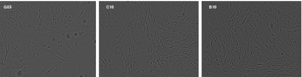
Scientists often study images of the cells growing in the container (Figure2.1) to estimate the confluence and to decide whether or not to passage the cells. From a subjective viewpoint this is done by viewing the image and estimating the remaining space available for cell growth. This process is slow, manual, and highly variable, so being able to estimate the confluence directly from the image is an important capability of any automated cell growth platform. This estimation could be done, for example, by counting the number of cells, multiplying the number of cells by the average cell size and then comparing that area to the total surface area of the container. This approach is not generally desirable in an automated system because most methods to get this information kill the cells. A non-destructive way to get this information is through bright field imaging, where one shines a bright light down through the top of the container and records the image of the shadows from below. See Figure 2.2 for examples of bright field images.
However, to determine cell confluence level based on the shadows in a bright field image is difficult. One can hardly tell the cell number in the image explicitly. But some other visual factors in the image can help biologists make their assessment of confluence level, such as the shape of the cells (more accurately, the cell shadows), the amount of empty space for the cells to grow into and thecell path (the patterns in how the cells orient with respect to each other). Changes of these visual factors as the confluence level increases can be seen in Figure
2.2, where the three images are ordered from least confluent to most confluent. This manual assessment by biologists is usually subjective. Thus, it is proposed to develop a statistical approach to numerically summarize these visual features from an image and then make an objective statistical evaluation of cell confluence level.
Figure 2.2: Pre-processed and intensity-normalized bright field images of three different wells from a 96-well plate of adherent stem cells, sorted from low confluence level to high confluence level. The well names are on the upper left corner. The cells correspond to the long thin objects. From left to right, the cell number increases, the cell shape changes, the gap between cells gets smaller and the cells begin to orient with respect to each other.
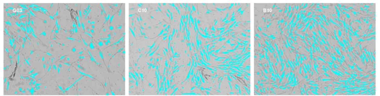
A single 96-well plate of adherent stem cells from a screening experiment by BD Tech-nologies is selected as the training sample. Each well is essentially a container in which cells are grown under a controlled condition. The culture conditions of the inner 60 wells rep-resent a variety of culture conditions that support different rates of cell growth, leading to different confluence levels. The passaging decisions will be made on the well level, i.e. the cells in the same well will be passaged together. A bright field image is taken for each of the inner 60 wells (Figure 2.2). The boundary of each cell is identified, that is, the cell is segmented, using a custom script developed at BD Technologies with IPLab for Pathway software (http://www.digitalimagingsystems.co.uk/software/iplab.html). Figure2.3
Pix-els that are identified to be interior to cells are colored cyan. The identified objects do not exactly cover the real cells, but this gives a useful approximation.
Figure 2.3: Cell identification (using IPLab imaging software) of the wells shown in Figure2.2. The well names are on the upper left corner. The cyan objects are the identified cells.
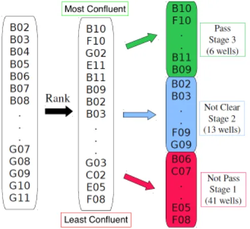
Since the confluence level cannot be directly and unambiguously determined in a bright field image, in order to get a confluence evaluation of the 60 wells, an experiment was designed where four biologists were asked to assess the confluence level of the 60 images. Figure 2.4
shows the work flow of this experiment. The images were initially ordered by well name, a random order of confluence level, as the condition of each well was chosen under a randomized design. At first the biologists participated in the experiment individually. Each of them sorted the images in order based on their own estimated confluence level γ, and then specified two thresholdsα1 and α2 (α1 > α2) for making a passaging decision for every image: to passage
ifγ > α1, not clear ifα2 < γ < α1, and not to passage ifγ < α2.
However, the evaluation results varied among biologists due to different subjective per-ceptions of confluence. After a careful discussion, the biologists finally reached a consensus assessment, referred to later asbio-assessment, which will be considered as an unbiased eval-uation of confluence level to judge the performance of the statistical approach developed later in Section 2.3. This assessment resulted in each image receiving an integer indicating the
Figure 2.4: Workflow of the manual assessment of confluence level. The images were originally ordered by name (B02, B03, ...), and then sorted in order of the estimated confluence by biologists. Finally the passaging decisions were made based on the estimated confluence level: to passage (high level), not clear (medium level) and not to passage (low level).
on subjective judgement, vary a lot among these experts.
Expert 1
Correlation with Consensus: 0.92 Agreement on Passaging: 43 %
Consensus Rank Individual Rank10
20 30 40 50 60
● ●
●
● ●
● ●
●
●
●
●
● ●
● ● ● ● ● ●
● ● ●
● ●
●
● ●
●
● ●
● ● ● ●
●
●
●
●
● ●
●
10 20 30 40 50 60
Expert 2
Correlation with Consensus: 0.84 Agreement on Passaging: 43 %
Consensus Rank Individual Rank10
20 30 40 50 60
● ●●
● ●
● ●
● ●
●
● ●
● ●
●
● ● ● ●
● ● ● ●
●
● ●
● ●
● ●
●
● ● ●
●
●
●
● ●
●
●
10 20 30 40 50 60
Expert 3
Correlation with Consensus: 0.81 Agreement on Passaging: 40 %
Consensus Rank Individual Rank10
20 30 40 50 60
● ● ●
●
● ●
● ●
●
●
● ●
●
● ● ● ● ● ●
● ●
● ●
●
●
● ●
●
●
● ● ● ● ●
●
●
●
● ●
●
●
10 20 30 40 50 60
Expert 4
Correlation with Consensus: 0.91 Agreement on Passaging: 72 %
Consensus Rank Individual Rank10
20 30 40 50 60
● ●
●
● ●
●
● ●
●
●
●
● ●
● ● ● ● ● ●
● ●
● ●
●
● ●
● ●
●
●
● ● ● ●
●
●
●
● ●
●
●
10 20 30 40 50 60
Figure 2.5: Graphical summaries of biologists evaluation of cell confluence level. Each panel corre-sponds to one biologist, and shows scatterplot of the individual rank of the wells vs. the consensus rank. The point color and symbol represent the consensus passaging decision: to passage (green squares), not to passage (red dots) and not clear (blue triangles). The wells whose individual passaging decision matches the consensus decision are highlighted in the boxes. The title shows the correlation between the individual and the consensus ranks and also the percentage of correct individual decisions (i.e. agreement on passaging).
which does not match the bio-assessment very well. It is shown later in Section 2.3.3 that the alternative statistical approach proposed in this chapter substantially improves the cell number assessment, in the sense of better predicting the bio-assessment.
2.2
Feature Extraction
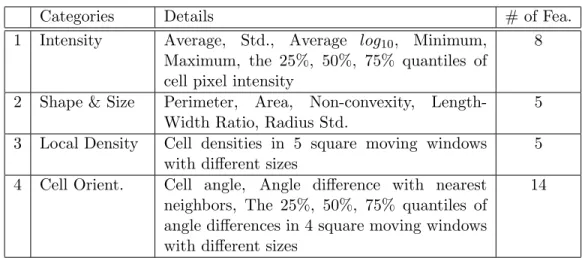
This section aims at numerically extracting cell confluence information from the bright field images. These images are carefully pre-processed beforehand. Some standard graphical tech-niques, such as flat field correction and convolution filter (Sternberg (1983)), are used to remove uneven background shading and granular noise. The pixel intensity is normalized across images. Two types of confluence-related features are extracted from the images:
(1) Cell features, including properties of an individual cell and its relationship with its neighbors. These features can be grouped into four categories, intensity, shape & size, local density, and cell orientation (cell path), as listed in Table 2.1.
(2) Entire-well features. Since cell confluence level is a function of the entire well instead of a simple collection of cells, some additional well-level, or image-level, features are also considered in evaluating confluence level. These well-level features, such as the cell number and some summaries of the gaps1 in the image, are summarized in Table 2.2.
These features are described in detail as follows. Due to irregular intensity distribution and irregular cell features respectively, two images are flagged as outliers.
2.2.1 Cell Features
The cell confluence generally involves two types of cell properties: (1) Individual properties, such as intensity, shape and size; (2) Relationship to neighboring cells, such as local density and angle pattern (how the cells orient with respect to each other). Those properties can be represented numerically ascell features(Table 2.1).
1
Table 2.1: Summary of cell features.
Categories Details # of Fea.
1 Intensity Average, Std., Average log10, Minimum,
Maximum, the 25%, 50%, 75% quantiles of cell pixel intensity
8
2 Shape & Size Perimeter, Area, Non-convexity, Length-Width Ratio, Radius Std.
5
3 Local Density Cell densities in 5 square moving windows with different sizes
5
4 Cell Orient. Cell angle, Angle difference with nearest neighbors, The 25%, 50%, 75% quantiles of angle differences in 4 square moving windows with different sizes
14
A cell identified by the IPLab imaging software can be expressed as a collection of pixels, or points, as shown in Figure2.6. Based on those pixels (bottom right), 32 cell features were computed, organized into the four groups as discussed below.
Figure 2.6: Cell identification in an IPLab segmented image. One identified cell is shown as the long diagonal cyan region contained completely in the upper right graph. The exact pixels in this highlighted cell are shown in the bottom right panel.
(1) Intensity
The cell intensity features are extracted from the intensity of the pre-processed and intensity-normalized bright field images. The darkness of the points in Figure 2.7 reveals the intensity pattern of the highlighted single cell in Figure 2.6. Some standard data sum-maries of the intensity in each cell, including mean, standard deviation, minimum, maximum and the 25%, 50%, 75% quantiles, are used as the intensity features of the cell. The average
log10 intensity is also calculated as a cell feature.
Figure 2.7: Intensity pattern of the highlighted cell in Figure2.6. Darkness codes the intensity.
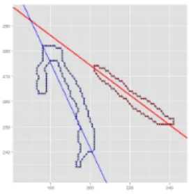
There are many ways to describe the shape and the size of a cell. Taking the highlighted cell in Figure 2.6as an example, the following features are considered in our study:
• Perimeter: The number of pixels at the cell boundary, indicated as the black dots in the first panel of Figure 2.8.
• Area: The number of pixels within a cell, i.e. the total number of points in Figure2.7.
• Non-convexity: Defined as Convex hull area −Cell area
Cell area . In the first panel of Figure 2.8,
the black polygon indicates the cell boundary, and the red polygon indicates the convex hull. The non-convexity is the ratio of the area (in pixel) of the gap between the red and the black polygons to the cell area (in pixel). A larger number indicates a less convex cell shape.
• Length-width ratio: The ratio between the first two eigenvalues of the PCA on pixel locations within a cell. In the second panel of Figure2.8, the green line and the blue line respectively indicate the first two principal component directions of the pixel locations of the cell. The length-width ratio is defined as the ratio between the pixel-location variances along these two directions. A larger number corresponds to a thinner shape.
• Standard deviation of radii. See the third panel of Figure 2.8 for details. The green point at the center is the mean point of the cell pixel locations. The radii are shown as the purple lines connecting the green point and the points at the cell boundary. The standard deviation of the length of these radii indicates how different the cell shape is from round.
Figure 2.8: Shape features of the highlighted single cell in Figure2.6. The black polygon indicates the cell boundary. Left: The convex hull of the cell boundary, shown in red. Middle: The first two principal component directions of the pixel locations of the cell, colored in green and blue respectively. Right: Radii of the cell centered at the mean of the cell pixel locations, colored in purple.
In order to study the local density of cells, square moving windows are used to define the neighborhood. For example, in Figure2.9, the black and the orange squares are two different windows for the central green cell, with side length 40 and 80 in pixel respectively. The blue objects are the neighbor cells. The local density of the green cell with respect to a certain window is defined as W indow areaT otal area of neighbor cells−Central cell area(blue(green) inside the window)inside the window. If the denominator is zero, then the local density is defined to be zero. Different window size leads to different local density distribution of an image. Here we used five different moving windows, with side length 20, 40, 80, 160, 320 in pixel respectively.
Figure 2.9: Zoomed-in view of a cell image. The black and the orange squares are two different windows to define different neighborhood areas of the central green cell, with side length 40 and 80 in pixel respectively. The neighbor cells are colored blue.
(4) Cell Orientation
in the second panel of Figure2.8, the cell orientation is represented by the green line. The [0,
π] angle between the this principal component direction and the horizontal line is defined as the cell angle. Then the angle difference between two cells (Figure 2.10) can be calculated. Since cells in a path have a similar orientation, a small angle difference among the neighbor cells usually indicates the existence of a cell path.
As discussed above, the angle difference between a cell and its nearest neighbor (measured by the distance between the centers of these two cells) is computed as an important feature of cell path. We also use four different moving windows (with side length 40, 80, 160, 320 in pixel respectively) to investigate the pattern of local cell orientation. Particularly, for each cell, the angle differences between the cell and its neighbors inside a certain window are computed, and the 25%, 50%, 75% quantiles of these angle differences are used to summarize the local cell orientation.
Figure 2.10: Angle difference between two cells. The red and the blue lines indicate the different cell orientations.
2.2.2 Entire-well features
As cell confluence level is a function of the entire well instead of a simple collection of cells, some additional well-level (or image-level) features also play an important role in evaluating cell confluence level, such as the number of cells. See Table2.2 for a brief summary of these features.
Thegapbetween cells refers to the non-cyan area in the IPLab segmented images (Figure
2.3). It is an important aspect to consider when evaluating cell confluence because of two main reasons:
Table 2.2: Summary of additional entire-well features.
Categories Details # of Fea.
1 Cell Number Number of identified cells in an image 1
2 Cell Gap Summaries* of gap intensity 6
Summaries* of the size of circular gaps** 6
*Standard deviation, min., max. and the 25%, 50%, 75% quantiles are used
as summaries.
**These features are extracted by performing the distance transformation
(Rosenfeld and Pfalz (1966)) on the IPLab segmented image. Statistical summaries of the intensity of the resulting distance image are used as a description of the size of the circular gaps among cells.
available for the cells to expand. Smaller gaps usually correspond a higher confluence level.
(2) As IPLab identification of cells (the cyan objects in Figure 2.3) cannot exactly cover the real cells, the gap contains part of the cell information.
These two facts respectively suggest two different properties of the gaps, the size and the intensity.
One way to highlight the gaps in an IPLab segmented image is to perform the distance
transformation, which maps each image to a new image called thedistance image. The pixel intensity of a distance image is proportional to the distance between the pixel and the nearest pixel inside the segmented cells. For example, in Figure 2.11, the blue objects represent the segmented cells. After distance transformation, the pixel intensity of the yellow point is proportional to the length of the red segment that connects the yellow point with the nearest blue point inside the segmented cells. Figure2.12shows the distance images that respectively correspond to the three IPLab segmented images in Figure2.3. The lighter color means that the pixel is farther from the segmented cells, which indicates a bigger circular gap. In this way, the distance images clearly displays the pattern of the gaps (light color) and the area of high cell density (dark area). Regular statistics of the intensity of distance images, such as standard deviation, minimum, maximum and the 25%, 50%, 75% quantiles, can be used as a summary of the size of the gaps.
Figure 2.11: A simple example to illustrate the distance transformation of an image. The pixel inten-sity of the yellow point in the resulting distance image is proportional to the length of the red segment.
Figure 2.12: The corresponding distance images of the three IPLab segmented images in Figure2.3.
images. Regular statistics of the gap intensity, such as standard deviation, minimum, maxi-mum and the 25%, 50%, 75% quantiles, are used.
2.3
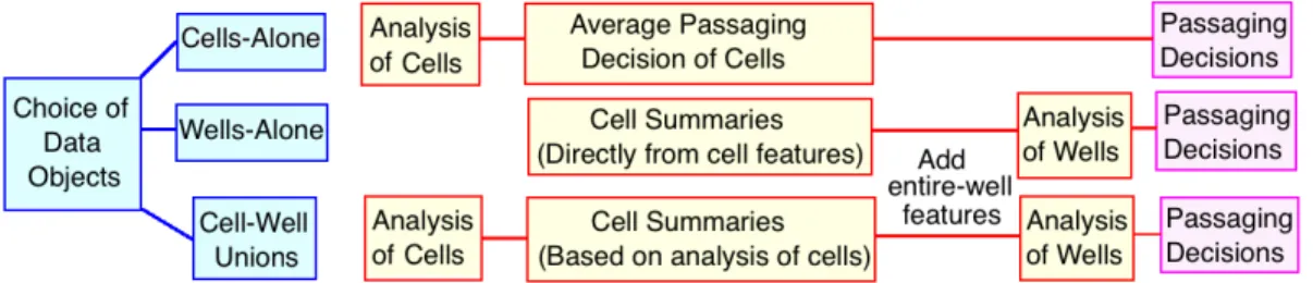
Object Oriented Data Analysis of Image Data
is the union of a well with its corresponding set of cells, or thecell-well unions. Section2.3.1
describes how the choice of data objects orients further analyses.
From an object-oriented point of view, the image data analysis is done in two steps: (1) Separate analyses for various choices of data objects (Section2.3.2), which show the advantage of treating the cell-well unions as data objects; (2) Analysis of cell-well unions as data objects (Section2.3.3), which provides the final results of our statistical assessment. See Section2.4
for further discussions of the choices of data objects.
2.3.1 Data Objects and the Consequential Analyses
As discussed in Section2.2, two different data sets are included in our analyses:
• Cell data(containing cell features of each individual cell);
• Well data (containing entire-well features of each well).
The cell sample size is always dramatically larger than the well sample size. The first challenge in analyzing cell-well structured data is how to combine these two data sets. One natural solution is to define statistics to summarize the cell features across wells, and then combine the summarized cell data with the well data. Finally, the statistical passaging decision for each well will be made based on the combined data set.
The following describes how the procedure of analysis will be oriented by the choice of data objects. Three different types of data objects and the corresponding data analyses are discussed.
(2) Wells-alone analysis, i.e. analysis based on wells alone as data objects. Both the cell data and the well data are used. However, since cells are not chosen as data objects, no cell data analysis is done here. The basic idea of this wells-alone analysis is to first summarize the cell features across wells directly by statistics, such as quantiles, and then combine the summarized cell data with the well data. Finally, the statistical passaging decisions are made by analyzing the combined data set.
(3) Cell-well union analysis, i.e. analysis based on cell-well unions as data objects. This analysis uses both the cell data and the well data. First, the cell data analysis finds an appropriate way to summarize the cell data across wells. In particular, it finds a linear combination of the cell features that correlates well with the bio-rank, and then takes statistics, such as quantiles, of this linear combination and its orthogonal PC scores across wells as the summarized cell data. Finally, the statistical passaging decisions are made based on the combined data set of the summarized cell data and the well data.
Figure 2.13: Workflows of three different analyses of cell images, oriented by different choices of data objects respectively. Summaries refer to statistics, such as quantiles, of the cell-level features.
data analysis into the cell summarization. See Section 2.4 for theoretical discussions of the choice of these data objects. It concludes that the cell-well unions are a better choice of data objects than the other two choices.
2.3.2 Comparison of Different Data Objects
This section aims at comparing the choices of three different data objects, the cells alone, the wells alone, and the cell-well unions, by performing the three corresponding analyses on the cell image data separately. For the purpose of comparison, we used the same statistical method, Distance Weighted Discrimination (DWD), to make the final passaging decisions in all these three analyses. Proposed by Marron et al.(2007), DWD is a powerful classification tool, especially for high dimensional cases. It was used here to find the best linear separations between pairs of the three passaging groups and then to predict the group labels as the predicted passaging decisions. The consensus bio-classification, described in Section2.1, will be considered as a gold standard to judge the performance of these analyses.
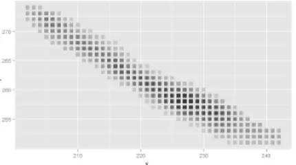
(1) Cells-alone analysis. Figure2.14 (left) visualizes the cell data in two dimensions using Principal Component Analysis (PCA). The point color and the symbol are determined by the bio-assessment. The unclear pattern of either the colors or the symbols suggests that the confluence information contained in the cell data is not obvious. We intended to use DWD to classify the cell data directly. Each cell in a well would receive a label indicating its predicted passaging group, and the passaging decision for this well would be predicted by the average label of the cells within this well. However, due to the large sample size of the cells (over 20,000), we encountered computational difficulties using the current DWD R package by Huang et al. (2012). As an alternative approach, we randomly sampled the wells and randomly sampled a small set of cells from each well, and then used DWD to classify this smaller data set. This procedure was repeated 500 times, and the average classification error rate was 25.1%.