GEOSTATISTICAL DATA FUSION ESTIMATION METHODS OF AMBIENT PM2.5 AND POLYCYCLIC AROMATIC HYDROCARBONS
Jeanette M. Reyes
A dissertation submitted to the faculty at the University of North Carolina at Chapel Hill in partial fulfillment of the requirements for the degree of Doctor of Philosophy in the Department of Environmental Sciences
and Engineering in the Gillings School of Global Public Health.
Chapel Hill 2016
ABSTRACT
Jeanette M. Reyes: Geostatistical Data Fusion Estimation Methods of Ambient PM2.5 and Polycyclic Aromatic Hydrocarbons
(Under the direction of Marc L. Serre)
Fine Particulate Matter (PM2.5) is a complex air pollutant associated with a host of adverse health effects. In epidemiologic studies there is a need to accurately predict exposures to reduce
misclassification. Recently there has been a surge in data fusion methods which combine observed data with gridded modeled data like the regulatory Community Multiscale Air Quality (CMAQ) model.
Substantial resources are allocated to the evaluation of CMAQ. However, this model has inherent error and uncertainty. Currently, CMAQ can only be operationally evaluated at locations where observed data exist, leaving potentially large spatial and temporal gaps in a given modeling domain. This study develops a framework for evaluating gridded air quality modeled data that can then be corrected for systematic error and combined with observed data in a geostatistical framework. First, this dissertation develops the novel Regionalized Air quality Model Performance (RAMP) method that performs a non-homogenous, non-linear, non-homoscedastic model evaluation at each CMAQ grid for a well-documented 2001 regulatory episode across the continental United States. The RAMP method comparatively outperforms other model evaluation methods with a 22.1% reduction in Mean Square Error (MSE). Secondly, the RAMP corrected CMAQ modeled data are combined with observed data in the modern Bayesian Maximum Entropy (BME) geostatistical framework which combines the accuracy of observed data with the spatial and temporal coverage of gridded modeled data. RAMP BME resulted in a 6-7 times increase in spatial refinement compared to using kriging alone. Lastly, the data rich PM2.5 environment is
contrasted with the data poor environment of Polycyclic Aromatic Hydrocarbons (PAHs). The Mass Fraction (MF) BME method is developed through a relatively small number of paired PM2.5 and PAH values and is applied to PM2.5 observed locations where PAH have not been observed to create the first detailed spatial maps of PAH across North Carolina in 2005. The MF BME method reduces MSE by over 39% compared with using kriging alone. Accurate assessment of ambient air pollutants is essential in
public health to explore and elucidate true underlying relationships between pollutants and health endpoints.
v
ACKNOWLEDGMENTS
First and foremost, I would like to thank my advisor, Dr. Marc Serre, for his constant guidance and counsel. His mentorship throughout the years has taught me life-long lessons about research, technical writing, public health and professional collaborations. I would like to thank Dr. William Vizuete for his guidance in the WHIMS project along with his technical background and expertise with
atmospheric chemistry. I would also like to thank my committee members Dr. Michael Flynn, Dr. Amy Herring and Dr. Joachim Pleil for their thoughtful and poignant comments that guided this dissertation.
Along with those at UNC, I would like to thank mentors at the EPA, especially Dr. Ana Rappold, Dr. Lisa Baxter and Dr. Lucas Neas for providing additional insight and research opportunities that both directly and indirectly bolstered this work.
I would like to thank past and present members of the BME lab for their insights and discussions including Dr. Yasuyuki Akita and Prahlad Jat along with my co-author for this work, Dr. Yadong Xu.
Lastly, I would like to thank all my friends and family for their support and their constant convincing that this work would be completed.
I would like to acknowledge the National Institute on Aging (NIA) under award number
vi
TABLE OF CONTENTS
LIST OF TABLES ... ix
LIST OF FIGURES ... x
CHAPTER 1: INTRODUCTION ... 1
CHAPTER 2: REGIONALIZED PM2.5 COMMUNITY MULTISCALE AIR QUALITY MODEL PERFORMANCE EVALUATION ACROSS A CONTINUOUS SPATIOTEMPORAL DOMAIN ... 5
2.1 Introduction... 5
2.2 Materials and Methods ... 7
2.2.1 Observed and Modeled Data ... 7
2.2.2 Variable Definition ... 7
2.2.3 Systematic and Random Error Statistics ... 7
2.2.4 Constant Air quality Model Performance (CAMP) ... 8
2.2.5 Regionalized Air quality Model Performance (RAMP) ... 9
2.3 Results and Discussion ... 13
2.3.1 Model Performance Evaluation Results Demonstrating the RAMP Analysis ... 13
2.3.2 Validation Results ... 15
2.3.3 Stochastic Simulation Results ... 17
2.3.4 Evidence and Implications of Non-Linear and Non-Homoscedastic Model Performance ... 18
2.3.5 Spatial Patterns of Systematic and Random Errors ... 19
2.4 Conclusions ... 21
CHAPTER 3: INCORPORATING REGIONALIZED AIR QUALITY MODEL PERFORMANCE EVALUATION IN A NATIONWDIE GEOSTATISTICAL DATA INTEGRATION OF DAILY PM2.5 ... 23
3.1 Introduction... 23
3.2 Materials and Methods ... 25
3.2.1 Observed and modeled data ... 25
3.2.2 BME estimation methodology ... 25
3.2.3 Regionalized Air quality Model Performance (RAMP) soft data construction ... 26
3.2.4 Leave One Out Cross Validation (LOOCV) accuracy analysis ... 27
3.2.5 Comparison to the frequentist Downscaler method ... 28
3.3 Results and Discussion ... 29
vii
3.3.2 Validation results ... 31
3.3.3 Non-homogenous behavior of BME data fusion ... 34
3.3.4 Stratification of BME data fusion performance ... 37
3.3.5 Data fusion corrects the bias of observation based predictions ... 37
3.3.6 Data fusion captures fine scale variability of PM2.5 ... 38
3.3.7 Overall contributions and future works ... 40
CHAPTER 4: INCORPORATING MASS FRACTION OF POLYCYCLIC AROMATIC HYDROCARBONS INTO THE BAYESIAN MAXIMUM ENTROPY FRAMEWORK ACROSS NORTH CAROLINA ... 41
4.1 Introduction... 41
4.2. Materials and Methods ... 43
4.2.1 Observed PM2.5 and PAH data... 43
4.2.2 The Mass Fraction (MF) and Linear Regression (LR) method ... 43
4.2.3 Soft data neighborhood validation optimization ... 44
4.2.4 Bayesian Maximum Entropy (BME) estimation methodology ... 45
4.2.5 Leave One Out Cross Validation (LOOCV) accuracy analysis ... 46
4.2.6 Fire comparisons ... 47
4.3. Results and Discussion ... 47
4.3.1 Neighborhood optimization ... 47
4.3.2 PAH prediction maps ... 49
4.3.3 Cross-validation ... 51
4.3.4 Probability of exceedance ... 53
4.3.5 Association with fires ... 56
4.3.6 Overall contributes and concluding statements ... 57
CHAPTER 5: CONCLUDING REMARKS ... 59
APPENDIX A: SUPPORTING INFORMATION FOR REGIONALIZED PM2.5 COMMUNITY MULTISCALE AIR QUALITY MODEL PERFORMANCE EVALUATION ACROSS A CONTINUOUS SPATIOTEMPORAL DOMAIN ... 61
A.1 Model Performance Metrics ... 61
A.2 Data ... 63
A.2.1 Observed Data... 63
A.2.2 Modeled Data ... 64
A.3 Choice of S-Curve Parameters for the RAMP analysis ... 64
A.4 Model Performance Metrics for Different Fixed Modeled Values ... 66
A.5 Maps of Other Model Performance Metrics ... 67
A.6 𝝀𝟏(𝒙𝒌; 𝓡(𝒑)) and 𝝀𝟐(𝒙𝒌; 𝓡(𝒑)) for Different Fixed Modeled Values ... 68
viii
APPENDIX B: SUPPORTING INFORMATION FOR INCORPORATING REGIONALIZED AIR QUALITY MODEL PERFORMANCE EVALUATION IN A NATIONWDIE
GEOSTATISTICAL DATA INTEGRATION OF DAILY PM2.5 ... 75
B.1 Offset and Covariance Optimization ... 75
B.2 Quantification of Spatial Refinement ... 79
B.3 Implementation of the Frequentist Downscaler Method ... 82
B.3.1 Equations ... 82
B.3.2 Empirical Estimation of Parameters ... 82
B.3.3 Development of the Predictive Distribution ... 83
B.3.4 Development of the Distribution of the bias (additive and multiplicative) ... 84
APPENDIX C: SUPPORTING INFORMATION FOR INCORPORATING MASS FRACTION OF POLYCYCLIC AROMATIC HYDROCARBONS INTO THE BAYESIAN MAXIMUM ENTROPY FRAMEWORK ACROSS NORTH CAROLINA ... 85
APPENDIX D: WHIMS CODE DOCUMENTATION AND QUALITY ASSURANCE FOR THE ESTIMATION OF PM2.5 AFTER 1999 USING OBSERVATION AND CTM ... 89
D.1 Introduction ... 89
D.2 Materials ... 89
D.2.1 PM2.5 daily data ... 89
D.2.2 PM2.5 Modeled Data ... 91
D.3 Methods ... 92
D.3.1 Estimation of Daily PM2.5 Concentration ... 92
D.4 Numerical implementation ... 93
D.4.1 Data and analysis folders ... 93
D.4.2 Instructions to estimate PM2.5 concentration after to 1999 ... 94
D.5 Results ... 95
D.6 QAQC ... 95
D.7 Date and version number ... 96
APPENDIX E: GITHUB URL ... 97
ix
LIST OF TABLES
Table 2.1. Validation statistics... 17
Table 3.1. Cross validation statistics ... 36
Table 4.1. Soft data neighborhood optimization ... 47
Table 4.2. Cross validation statistics ... 51
Table 4.3. Mean difference in PAH near versus far from fires ... 55
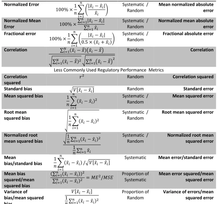
Table A.1. Table of commonly used model performance evaluation statistics used in the CMAQ literature ... 61
Table A.2. Table of model performance evaluation statistics used when the estimate xi has a corresponding variance σi2 ... 62
Table A.3. Ranking scores used for averaging collocated PM2.5 values for a given site/day ... 64
Table A.4. Description of available CMAQ modeling data ... 64
Table B.1. Offset parameter values and namings used to smooth PM2.5 in space/time ... 76
Table B.2. Covariance model and parameter values for each offset calculated through least squares fitting ... 78
Table B.3. Spatial covariance ranges of the posterior means of the boxed regions ... 81
Table C.1. Covariance model parameters for observed PAH data... 85
Table C.2. Cokriging covariance model parameters for observed PAH and PM2.5 data ... 86
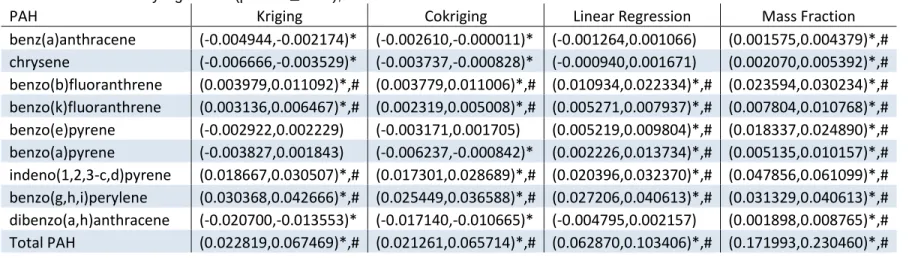
Table C.3. Cross validation statistics for all 9 PAHs and Total PAH ... 87
Table D.1. Folder Directory for WHIMS ... 94
Table D.2. Shell scripts to run for each folder ... 95
x
LIST OF FIGURES
Figure 2.1. Visual representations of systematic and random error ... 11
Figure 2.2. Maps of RAMP error and RAMP error correction of CMAQ ... 15
Figure 2.3. Map of RAMP mean error ... 21
Figure 3.1. Map of kriging and BME mean and variance ... 31
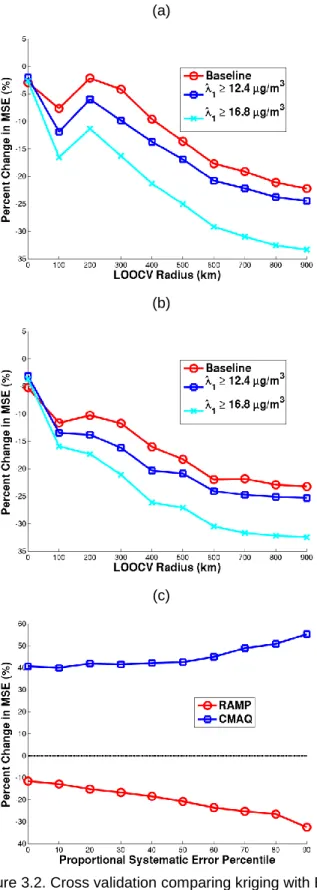
Figure 3.2. Cross validation comparing kriging with BME and the frequentist Downscaler... 33
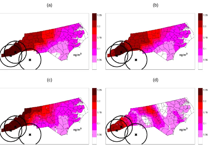
Figure 4.1. Map of benzo(g,h,i)perylene ... 49
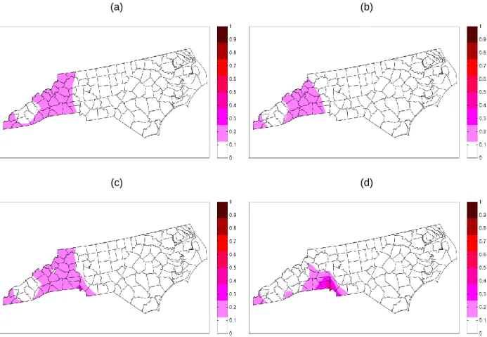
Figure 4.2. Probability of exceedance ... 53
Figure 4.3. PAH ratios ... 57
Figure A.1. Maps of λ1(p) and λ2(p) across the US on July 1, 2001 calculated using the RAMP method with two sets of S-curve parameters ... 66
Figure A.2. Systematic error ... 67
Figure A.3. Random error ... 67
Figure A.4. Maps of various metrics across the continental United States on 07/01/2001 ... 68
Figure A.5. Maps of λ1(xk; R(p)) ... 69
Figure A.6. Maps of λ2(xk; R(p)) ... 70
Figure A.7. Maps of stochastic simulation of daily PM2.5 across the continental United States on 07/01/2001 ... 72
Figure A.8. (a) Map of the selected true MEp = xp − λ1(p) for daily PM2.5 across the continental United States on 07/01/2001, and maps of the corresponding re-estimated ME ∗ p = xp − λ1 ∗ (p) ... 73
Figure A.9. (a) Map of the selected true VEp = λ2(p) for daily PM2.5 across the continental United States on 07/01/2001, and maps of the corresponding re-estimated VE ∗ p = λ2 ∗ (p) ... 74
Figure B.1. PM2.5 concentration across the continental US on July 30, 2001 after smoothing the data .. 76
Figure B.2. Time series of PM2.5 concentration across an arbitrary PM2.5 monitoring station ... 77
Figure B.3. Experimental and modeled covariance of the transform of the short, intermediate, long and very long offset ... 77
Figure B.4. Dominance plots ... 78
Figure B.5. Posterior mean of PM2.5 across the contiguous US on July 1, 2001 ... 79
xi
1
CHAPTER 1: INTRODUCTION
Epidemiologic studies investigating long term health effects of ambient air pollution exposures require accurate assessments to properly investigate underlying associations and health measures. Substantial efforts from sophisticated models have been used in past works to reduce misclassification that can otherwise obfuscate associations. The work presented here improves upon existing methods of exposure assessment. This work performs a model performance evaluation of gridded modeled
Particulate Matter ≤ 2.5 micrometers (PM2.5) data across the continental United States (US) in 2001 which is then corrected of systematic error. The corrected modeled data is combined with observed PM2.5 data in the Bayesian Maximum Entropy (BME) geostatistical framework. Lastly, this work ends with the estimation of Polycyclic Aromatic Hydrocarbons (PAHs) across North Carolina in 2005. This is the first known work to create a flexible data fusion method combining observed and gridded modeled data for PM2.5 using the BME framework. This is also the first known work to create a full prediction map of PAH across North Carolina for 2005. We hypothesize that combining environmental air pollution data sets defined over different supports (i.e. over a point location versus over a grid) in a geostatistical framework will improve estimation accuracy compared to using a single data source for a given environmental parameter.
Model performance evaluation is needed to understand resulting model error and in an
epidemiologic context when the resulting gridded estimations are being used to estimate exposure. There is a wealth of studies that explore performance evaluation of gridded Chemical Transport Models (CTMs), specifically the Community Multiscale Air Quality (CMAQ) model. CMAQ is the US Environmental
performance are numerous and multifaceted. These metrics becomes increasingly difficult to properly calculate when the region over which they are being calculated becomes increasingly smaller in size (Simon et al., 2012). Currently, an operational performance cannot be assessed in-between monitors and, in the limiting case, cannot be assessed for individual CMAQ grids. This information is needed to assess performance in-between monitors and to perform an error correction on individual CMAQ grids.
Most epidemiologic studies utilize data fusion methods. In recent years, these methods have increased in popularity. Data fusion methods typically combine two different data sources of a given air pollutant, where the data sources have different levels of support into a geostatistical framework. Different supports typically include observed monitoring data defined at a point location with modeling data defined over a grid. Data fusion methods allow for the accuracy typically associated with observed data with the spatial refinement and coverage associated with gridded modeling data. Popular approaches include Bayesian Melding and the Downscaler method (Berrocal et al., 2010a; Fuentes and Raftery, 2005). As sophisticated as these models can be, they still assume the relationship between modeled and observed data to be linear and homoscedastic. This can be limiting when there is a known difference between uncertainties of errors for difference ranges of PM2.5 concentrations. There are a variety of geostatistical methods that can implement a data fusion framework, including the BME framework.
BME is a mathematically rigorous geostatistical space/time framework originally developed by Christakos (Christakos and Serre, 2000; Christakos et al., 2001). BME is an extension of linear kriging in which information about a Space/Time Random Field (S/TRF) is divided into two knowledge bases: 1) a site-specific knowledge base characterizing the Space/Time Random Field (S/TRF) representing a process at a specific space/time, 2) a general knowledge base that comes in the form of a prior Probability Distribution Function (PDF) describing the random field. These knowledge bases are
combined and the BME posterior PDF can be used to predict environmental parameters at unmonitored locations. Unlike kriging, BME is able to incorporate information that is non-Gaussian. In an
environmental setting this can be essential when the distribution of the parameter is known to be highly skewed, when a sizable portion of a PDF is below zero, or when parameters are below a given detection limit (Messier et al., 2015). BME has been successfully implemented in water (Akita et al., 2007), air (Reyes and Serre, 2014) and disease parameters (Allshouse et al., 2011). BME data fusion has been
3
performed with ozone in previous work (de Nazelle et al., 2010; Xu et al., 2016). BME can also be used to inform mapping scenarios in data poor environments.
PM2.5 is a complex mixture of many different constituents. A component of PM2.5 is PAH. PAHs are created from incomplete fuel combustion with some species being carcinogenic (Bocskay et al., 2005; Menzie et al., 1992; Wolff et al., 2005). They can come from a variety of sources including wildfires. However, ambient PAHs are currently not regulated by the EPA and therefore, a nationwide monitoring network does not currently exist for them. PAH measurements can also be costly (Pleil et al., 2004). There is a need to investigate PAH concentrations over a large region in a cost effective way. Previous work has investigated the relationship between PAH and PM2.5 concentration around the World Trade Center after September, 11th (Allshouse et al., 2009). In particular, PM2.5 samples were analyzed for several different species of PAH. The relationship between the fractions of PAH to PM2.5 was investigated and applied to other areas in the sampling region. However, this was only applied to a relatively small region over a short period of time. Maps of PAH concentrations across North Carolina are currently lacking in the literature.
4
5
CHAPTER 2: REGIONALIZED PM2.5 COMMUNITY MULTISCALE AIR QUALITY MODEL PERFORMANCE EVALUATION ACROSS A CONTINUOUS SPATIOTEMPORAL DOMAIN1 2.1 Introduction
Particulate Matter ≤ 2.5 micrometers in diameter (PM2.5) is one of the six “criteria air pollutants” regulated in the United States (Boldo et al., 2006; Pope et al., 2009) due to its association with adverse health effects, including cardiovascular and respiratory disease and mortality (Beelen et al., 2007; Krewski et al., 2009; Pope et al., 2004). The Community Multiscale Air Quality (CMAQ) model is used for regulatory purposes to estimate PM2.5 and assess attainment. Substantial efforts are made to assess and understand the model performance of CMAQ ensuring that modeled values match with observed data (Appel et al., 2013b, 2008; Carlton et al., 2010; Foley et al., 2015a, 2015b, 2010). Past work evaluating model performance typically gives modeling performance statistics over an aggregated level (e.g. monitoring locations, regions of the country, monitoring networks, etc.) (Simon et al., 2012). For the modeling domain of the continental United States, metrics are typically calculated for the Eastern versus Western US, urban stations versus rural stations, summer versus winter monitoring, etc. (Appel et al., 2013a). Displaying model performance metrics at each monitoring site location across the US reveals that CMAQ performance changes in a non-homogenous manner (Appel et al., 2012). However, model
performance at a specific unmonitored space/time location is typically not explored or known. Therefore current methods fail to assess geographical or temporal changes of model performance across the spatiotemporal continuum, particularly in-between monitors.
The goal of this work is to address this significant knowledge gap by introducing a method that assesses model performance at any space/time region of interest across the spatiotemporal continuum.
1This chapter was submitted as an article to the journal Atmospheric Environment. Reyes, Jeanette M.,
Advantages for assessing model performance at any region across a continuum include being able to 1) exactly delineate geographical patterns of modeling errors and 2) correct systematic errors across the modeling domain for individual CMAQ grid concentrations.
Systematic errors are consistent deviations of modeled data from observed data. Systematic errors, once assessed, can be used to correct the modeled value. The remaining error, i.e. the random noise of the modeled value around the observed data, is the random error. While current CMAQ model performance evaluation methods are multifaceted (Dennis et al., 2010) and use a wide array of metrics to quantify performance (Kang et al., 2007; Thunis et al., 2012; USEPA, 2005; Venkatram, 2008), this work specifically focuses on set of metrics that investigate systematic and random errors. Hence, to achieve our goal, we introduce modeling error statistics that parse total errors into systematic and random errors. Few studies have apportioned error in this manner (Solazzo and Galmarini, 2016).
The method we introduce in this work to assess model performance across the spatiotemporal continuum is the Regionalized Air quality Model Performance (RAMP) method, which we use to study daily PM2.5 across the continental US. Our framework is a regionalized space/time extension of the Constant Air quality Model Performance (CAMP) method (de Nazelle et al., 2010) and parallels the work of Xu et al. (Xu et al., 2016). The CAMP method was originally used to account for the non-linear and non-homoscedastic relationship between modeled and observed ozone data in North Carolina for a particular ozone episode. The CAMP method assumes that model performance is homogenous across the state and does not change as a function of the space/time CMAQ grid locations. This assumption of homogeneity of model performance begins to break down as the modeling domain increases in size, particularly when this increase is substantial. The novel RAMP method introduced here for PM2.5 extends the CAMP method by accounting for the non-homogeneity of model performance in a
regionalized fashion across the entirety of a modeling domain and fully characterizes the non-linear and non-homoscedastic relationship at any space/time region for any modeled value of interest.
This work demonstrates the use of the RAMP method by implementing a regionalized
performance evaluation of daily PM2.5 mass predicted by CMAQ across the entirety of the continental United States. As an evaluation of the RAMP method, we have chosen a regulatory episode developed for the years 2001 and 2002. The model performance for this episode has been well documented and
7
thus provides an ideal case study of the RAMP method. The results of the RAMP analysis include maps showing the geographical variations of systematic and random errors at a fine spatial resolution displayed at the resolution of an individual CMAQ grid cell. These results provide new insights regarding model performance that complement existing performance evaluation methods. The RAMP results are helpful in making decision on resource allocation for further improvement in the air quality model. Furthermore, calculating systematic errors for individual CMAQ grids facilitate systematic error correction leading to maps of PM2.5 concentrations with improved mapping accuracy.
2.2 Materials and Methods
2.2.1 Observed and Modeled Data
Daily observed PM2.5 for each space/time location during 2000-2002 were constructed based on raw monitoring data from monitoring stations measuring either hourly or daily PM2.5 obtained from the EPA’s Air Quality Systems (AQS) data base (US EPA, n.d.). Daily PM2.5 data were also constructed from CMAQ modeled data for years 2001 and 2002 using CMAQv4.5 across the contiguous United States on a 36 km grid. For more detailed information regarding the aggregation and pairing process of observed and modeled data see Appendix A.
2.2.2 Variable Definition
Random variables 𝑋 are in upper case and known values are in lower case. Let 𝑋̂(𝒑) be the random variable representing the observed concentration at a single space/time location 𝒑 = (𝒔, 𝑡), 𝑥̂(𝒑) be its known value (i.e. realization) at space/time location 𝒑 and 𝑥̃(𝒑) be the CMAQ modeled value at space/time location 𝒑. Because 𝑥̃(𝒑) covers the entirety of the domain, it is known everywhere. We define error as
𝐸(𝒑) = 𝑥̃(𝒑) − 𝑋̂(𝒑) (Equ. 2-1)
Error is defined as 𝑒(𝒑) = 𝑥̃(𝒑) − 𝑥̂(𝒑) at locations where the observed data are known. The definition of error in this work is a deviation from what is typically used in the model performance literature. The differences in the nomenclature are explicitly stated in Appendix A (Table A.1 and Table A.2). 2.2.3 Systematic and Random Error Statistics
8
and modeled CMAQ data and can be removed through calculating the mean systematic error. Random errors are the residual errors remaining once the systematic error is removed. Random errors can be conceptualized as the random noise between CMAQ and observed data. Total error is the sum of systematic and random error. In the naming convention of a statistic the first letter(s) is used to identify the statistical operator as follows: M=mean, V=variance, S=Standard deviation, RMS=square Root of the Mean of Squared values. The last letter(s) is used to identify the value of interest as follows: E=Error (Equ. 2-1), SE=Squared Error=𝐸2, S=Standardized error=𝐸/𝜎
𝐸, NE=Normalized Error=E/𝑥̂ and R=square Root of error variance=√𝜎𝐸. Statistics that are calculated over an entire domain 𝒟 are 𝑀𝐸(𝒟) = 1
𝑛(𝒟)∑ 𝑒𝑖 and 𝑉𝐸(𝒟) = 1
𝑛(𝒟)−1∑(𝑒𝑖− 𝑀𝐸(𝒟))
2. 𝑀𝐸2(𝒟) quantifies the systematic error, 𝑉𝐸(𝒟) quantifies the
random error and 𝑀𝑆𝐸(𝒟) = 𝑀𝐸2(𝒟) + 𝑉𝐸(𝒟) quantifies the total error. The equations of systematic, random and total error can be represented pictorially through use of a target analogy, probability
distribution function of error and plotting observed data as a function of modeled data (Fig. 2-1a-i). Other statistics used in model performance evaluation include the square Root of the Mean of Squared
Standardized errors (RMSS) and Mean of the square Root of variance (MR). 2.2.4 Constant Air quality Model Performance (CAMP)
The CAMP method (de Nazelle et al., 2010) performs a model performance analysis that
accounts for the non-linearity and non-homoscedastic behavior of model performance with respect to the modeled value 𝑥̃𝑘. The CAMP method does this by modeling the mean 𝜆1(𝑥̃𝑘; 𝒟) = 𝑀[𝑋̂|𝑥̃𝑘; 𝒟] and variance 𝜆2(𝑥̃𝑘; 𝒟) = 𝑉[𝑋̂|𝑥̃𝑘; 𝒟] of the observed value 𝑋̂ as function of a given model value 𝑥̃𝑘 across the domain 𝒟 using the equations
𝜆1(𝑥̃𝑘; 𝒟) ≈ 1
𝑛(𝑥̃𝑘;𝒟)∑ 𝑥̂𝑖 (Equ. 2-2)
𝜆2(𝑥̃𝑘; 𝒟) ≈ 1
𝑛(𝑥̃𝑘;𝒟)−1∑(𝑥̂𝑖− 𝜆1(𝑥̃𝑘; 𝒟)) 2
(Equ. 2-3) where 𝑛(𝑥̃𝑘; 𝒟) is the number of paired modeled 𝑥̃𝑖 and observed 𝑥̂𝑖 values across the space time domain 𝒟 such that 𝑥̃𝑘− ∆𝑥̃ ≤ 𝑥̃𝑖≤ 𝑥̃𝑘+ ∆𝑥̃ where ∆𝑥̃ is a small tolerance corresponding to half of a decile of modeled values.
9
performance is non-linear and non-homoscedastic. However the CAMP method does not investigate how 𝜆1(𝑥̃𝑘; 𝒟) and 𝜆2(𝑥̃𝑘; 𝒟) S-curves change across space and time.
2.2.5 Regionalized Air quality Model Performance (RAMP)
The Regionalized Air quality Model Performance (RAMP) method introduced here consists of extending the CAMP method (de Nazelle et al., 2010) by regionalizing the model performance to a space/time region ℛ(𝒑) associated with the space/time coordinate 𝒑. In this work the region ℛ(𝒑) was selected such that it contains all paired modeled and observed data from the 3 closest stations within 180 days of 𝒑, resulting in a regionalized S-curve (Fig. 2-1j). The 3 closest stations within 180 days were chosen for being as spatially specific as possible while still maintaining a stable pattern with the
associated regionalized 𝜆1(𝑥̃𝑘; ℛ(𝒑)) = 𝑀[𝑋̂|𝑥̃𝑘; ℛ(𝒑)] and 𝜆2(𝑥̃𝑘, ℛ(𝒑)) = 𝑉[𝑋̂|𝑥̃𝑘; ℛ(𝒑)] parameters (see Appendix A for S-curve parameter optimization). The parameters are calculated as
𝜆1(𝑥̃𝑘; ℛ(𝒑)) ≈ 1
𝑛(𝑥̃𝑘;ℛ(𝒑))∑ 𝑥̂𝑖 (Equ. 2-4)
𝜆2(𝑥̃𝑘; ℛ(𝒑)) ≈ 1
𝑛(𝑥̃𝑘;ℛ(𝒑))−1∑(𝑥̂𝑖− 𝜆1(𝑥̃𝑘; ℛ(𝒑)))
2
(Equ. 2-5) where 𝑛(𝑥̃𝑘; ℛ(𝒑)) is the number of paired modeled and observed points within ℛ(𝒑)and around 𝑥̃𝑘.
10
There is a correspondence between the parameters 𝜆1(𝑥̃𝑘; ℛ(𝒑)) and 𝜆2(𝑥̃𝑘; ℛ(𝒑)) and systematic and random errors. From Equ. 2-1 we have 𝑋̂ = 𝑥̃ − 𝐸, which, once substituted into 𝜆1(𝑥̃𝑘; ℛ(𝒑)) and 𝜆2(𝑥̃𝑘, ℛ(𝒑)) yields
𝜆1(𝑥̃𝑘; ℛ(𝒑)) = 𝑀[𝑥̃ − 𝐸 |𝑥̃𝑘; ℛ(𝒑)] = 𝑥̃𝑘− 𝑀[𝐸 |𝑥̃𝑘; ℛ(𝒑)] = 𝑥̃𝑘− 𝑀𝐸(𝑥̃𝑘; ℛ(𝒑)) (Equ. 2-6) 𝜆2(𝑥̃𝑘; ℛ(𝒑)) = 𝑉[𝑥̃ − 𝐸|𝑥̃𝑘; ℛ(𝒑)] = 𝑉[𝐸(𝒑)|𝑥̃𝑘; ℛ(𝒑)] = 𝑉𝐸(𝑥̃𝑘; ℛ(𝒑)) (Equ. 2-7) where 𝑀𝐸(𝑥̃𝑘; ℛ(𝒑)) and 𝑉𝐸(𝑥̃𝑘; ℛ(𝒑)) are the mean and variance, respectively, of the error associated with an arbitrary value 𝑥̃𝑘 predicted within region ℛ associated with 𝒑.
We also define 𝜆1𝑅𝐴𝑀𝑃(𝒑) = 𝜆1(𝑥̃(𝒑); ℛ(𝒑)) and 𝜆𝑅𝐴𝑀𝑃2 (𝒑) = 𝜆2(𝑥̃(𝒑); ℛ(𝒑)) as the mean and variance of observed concentration when 𝑥̃𝑘= 𝑥̃(𝒑), where 𝑥̃(𝒑) is the CMAQ modeled value at 𝒑. By replacing 𝑥̃𝑘 with 𝑥̃(𝒑) in Equ. 2-6 and Equ. 2-7, we obtain
𝜆1𝑅𝐴𝑀𝑃(𝒑) = 𝑥̃(𝒑) − 𝑀𝐸(𝑥̃(𝒑); ℛ(𝒑)) (Equ. 2-8)
𝜆𝑅𝐴𝑀𝑃2 (𝒑) = 𝑉𝐸(𝑥̃(𝒑); ℛ(𝒑)) (Equ. 2-9)
Equ.2-8 and Equ. 2-9 provide a physical interpretation of systematic and random errors. The systematic error 𝑀𝐸(𝑥̃(𝒑); ℛ(𝒑)) is the error correction that can be applied to the modeled value 𝑥̃(𝒑) in region ℛ(𝒑) to produce a corrected modeled estimate 𝜆1𝑅𝐴𝑀𝑃(𝒑), and the random error quantified by 𝑉𝐸(𝑥̃(𝒑); ℛ(𝒑)) characterizes the residual uncertainty associated with the systematic error-corrected modeled estimate. In this work 𝑀𝐸(𝑥̃(𝒑); ℛ(𝒑)) and 𝑉𝐸(𝑥̃(𝒑); ℛ(𝒑)) can be approximated by 𝑀𝐸(𝑥̃(𝒑); ℛ(𝒑)) ≈ 1
𝑛(𝒑)∑ 𝑒𝑖 and 𝑉𝐸(𝑥̃(𝒑); ℛ(𝒑)) ≈ 1
𝑛(𝒑)−1∑(𝑒𝑖− 𝑀𝐸(𝑥̃(𝒑); ℛ(𝒑)))
2, respectively, where for a given 𝒑, 𝑛(𝒑) is equal to the
number of paired modeled and observed points in ℛ(𝒑).
The RAMP method provides the statistical distribution of observed air pollution as
𝑋̂(𝒑)|𝑥̃(𝒑)~𝑁(𝜆1𝑅𝐴𝑀𝑃(𝒑), 𝜆2𝑅𝐴𝑀𝑃(𝒑)) (Equ. 2-10)
11
ME2, VE ME2, VE ME2, VE
(a) (b) (c)
(d) (e) (f)
(g) (h) (i)
(j)
12
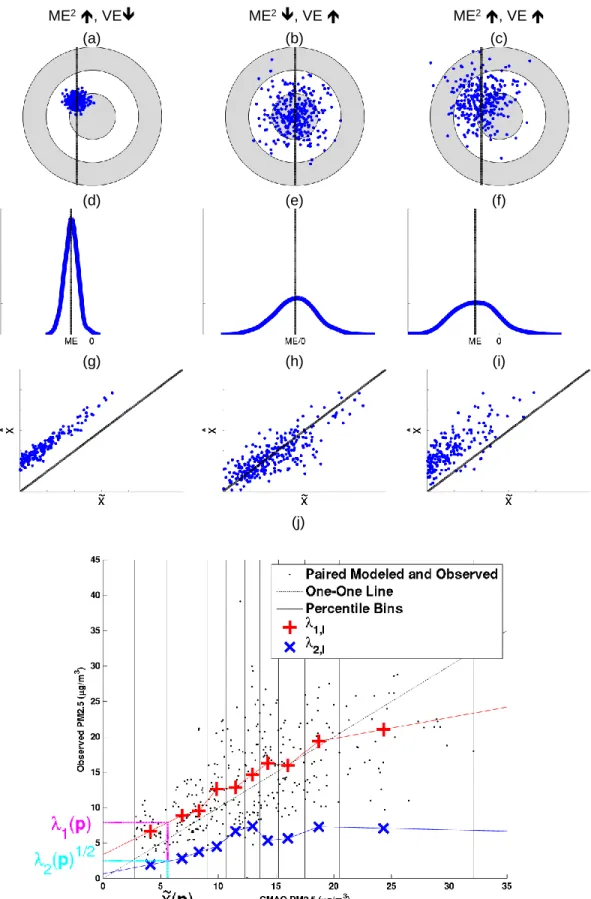
low VE). The middle column (plots (b), (e), (h)) displays representations of estimates with low systematic error and large random error. The right column (plots (c), (f), (i)) displays representations of estimates with large systematic error and large random error. The top row displays error using a target analogy, where estimates should ideally land on the target. The middle row displays the distribution of error via a PDF. The bottom row displays a group of paired modeled and observed concentrations around a given location. The modeled values are displayed on the independent axis as 𝑥̃ and the observed values are displayed on the dependent axis as 𝑥̂. The solid line is the one-to-one line. Plot (j) shows the RAMP analysis of an arbitrary CMAQ grid location on 07/01/2001 for daily PM2.5. The black dots are all the paired modeled and observed daily PM2.5 concentrations within a space/time region ℛ(𝒑) consisting of the 3 closest stations to the CMAQ grid location of interest within 180 days of 07/01/2001, with modeled data on the independent axis and observed data on the dependent axis. The vertical black lines identify the 10 bins used to stratify all the paired data in which each bin contains one decile of all the paired points. The dotted black line is the one-to-one line between the modeled and observed data. The red + marker in each bin denotes 𝜆1,𝑙(𝑥̃𝑙, ℛ(𝒑)), the average of paired observed values within the 𝑙-th decile bin. The blue x marker in each bin denotes the square root of 𝜆2,𝑙(𝑥̃𝑙; ℛ(𝒑)), the standard deviation of paired observed values within that bin. As shown in the figure, the + and x markers are linearly interpolated to obtain the 𝜆1(𝒑) and √𝜆2(𝒑) values, respectively, corresponding to the CMAQ modeled data 𝑥̃(𝒑) within ℛ(𝒑).
2.6 Validation and Stochastic Simulation
Validation is performed by comparing the accuracy of the model correction performed by three approaches: the Constant, CAMP, and RAMP correction methods. The Constant correction method is defined through
𝜆1𝐶𝑜𝑛𝑠𝑡𝑎𝑛𝑡(𝒑) = 𝑥̃(𝒑) − 𝑀𝐸(𝒟), (Equ. 2-11)
with associated error variance
𝜆𝐶𝑜𝑛𝑠𝑡𝑎𝑛𝑡2 (𝒑) = 𝑉𝐸(𝒟), (Equ. 2-12)
i.e. the correction 𝑀𝐸(𝒟) and its associated error variance 𝑉𝐸(𝒟) are constant across the entirety of the domain with respect to both modeled value 𝑥̃𝑘 and location 𝒑. The CAMP method assumes that the model performance of CMAQ is represented by domain wide S-curves 𝜆1(𝑥̃𝑘; 𝒟) and 𝜆2(𝑥̃𝑘; 𝒟) (Equ. 2-2,2-3) that are a function of the modeled value 𝑥̃𝑘, but not a function of space/time location 𝒑. In the CAMP method the correction for 𝑥̃(𝒑) is performed by substituting 𝑥̃𝑘 with 𝑥̃(𝒑) in the domain-wide S-curves, i.e. using the correction
𝜆1𝐶𝐴𝑀𝑃(𝒑) = 𝜆1(𝑥̃(𝒑); 𝒟) = 𝑥̃(𝒑) − 𝑀𝐸(𝑥̃(𝒑); 𝒟) (Equ. 2-13) with associated error variance
13
performance statistics between paired 𝜆1(𝒑) and 𝑥̂(𝒑)values for 2001. The performance of 𝜆2(𝒑) is assessed through standardized errors as shown in Table A.2 (i.e. 𝜆1(𝒑)−𝑥̂(𝒑)
√𝜆2(𝒑) ).
We also conduct a stochastic simulation to test how well each method reproduces the simulated truth. The maps of 𝜆1(𝒑) and 𝜆2(𝒑) obtained in this work are defined as being the true mean and variance of observed values. We also select 𝑥̃(𝒑) from this work as being the true modeled values. We randomly generate 𝑥̂∗(𝒑)~𝑁(𝜆1(𝒑), 𝜆2(𝒑)) and then we re-calculate 𝜆1∗
(𝒑) and 𝜆2∗(𝒑) using the Constant, CAMP and RAMP methods based only on paired 𝑥̃(𝒑) and 𝑥̂∗(𝒑). Lastly, 𝜆1∗
(𝒑) and 𝜆2∗(𝒑) are compared with 𝜆1(𝒑) and 𝜆2(𝒑) visually through maps and through statistical metrics to evaluate how well 𝜆1∗(𝒑) and 𝜆2∗(𝒑) are able to capture the spatial variability in the true mean, 𝜆1(𝒑), and variance, 𝜆2(𝒑), of observed values.
2.3 Results and Discussion
2.3.1 Model Performance Evaluation Results Demonstrating the RAMP Analysis
A demonstration of the RAMP method was performed using daily PM2.5 concentrations predicted by CMAQ at the 36 km grid level for 2001 across the continental United States. The version of CMAQ used to calculate the PM2.5 was v4.5, which is the most recent version of CMAQ available for 2001 across the continental US. Although newer versions of CMAQ exist for later years, it was critical to analyze model performance in 2001 due to an ongoing epidemiological study focused on novel
neurodegenerative PM2.5 health end points and its association with loss of brain mass in older women (Chen et al., 2015). This study is based on a cohort from the Women’s Health Initiative-Memory Study (WHI-MS) and exposure data was reconstructed from 1999 to 2006. From an epidemiologic perspective, a model performance evaluation that can distinguish systematic from random error is especially important for a model version with known deficiencies (Foley et al., 2010). This new information can inform
14
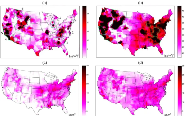
United States on that day. The maps shown in Fig. 2a-b allow for the identification of regions with high systematic and random errors. This is critical information needed to better understand the spatial
uncertainty of model performance of the CMAQ predicted values 𝑥̃(𝒑) across a given day (Fig. 2.2c). The RAMP analysis also produces 𝜆1𝑅𝐴𝑀𝑃(𝒑) (Fig. 2.2d), which can directly be used in place of CMAQ values. In addition to the results shown in Fig. 2.2, the RAMP analysis produces a rich set of more detailed model performance metrics (see Appendix A).
15
(a) (b)
(c) (d)
Figure 2.2. Maps of RAMP error and RAMP error correction of CMAQ. Daily PM2.5 across the continental United States on 07/01/2001 displaying (a) RAMP 𝑀𝐸2(𝒑), (b) RAMP 𝑉𝐸(𝒑), (c) CMAQ concentration 𝑥̃(𝒑) and (d) 𝜆1𝑅𝐴𝑀𝑃(𝒑). Plots (c) and (d) are in 𝜇𝑔/𝑚3 and (a) and (b) are in (𝜇𝑔/𝑚3)2. Plot (b) shows 6 regions of large random error delineated in the dashed green line with the same regions delineated and labeled in (a). Delineated regions include (1) the Great Lakes, (2) the Appalachian Mountains, (3) the South East, (4) Southern California, (5) Northern California and (6) the Rocky Mountains.
2.3.2 Validation Results
The validation statistics of three model performance evaluation methods (Constant, CAMP and RAMP) are shown in Table 2.1. These methods have increasing sophistication. The Constant method assumes that model performance is constant across 𝒟, the CAMP method accounts for non-linear and homoscedastic model performance and the RAMP method accounts for linear,
non-homoscedastic and non-homogeneous model performance shown in Table 2.1. The validation statistics are calculated using a corrected CMAQ value 𝜆1(𝒑) and associated error variance 𝜆2(𝒑) given by (Equ. 2-11, 2-12), (Equ. 2-13, 2-14), and (Equ. 2-8, 2-9) for the Constant, CAMP and RAMP methods,
respectively.
Validation of 𝜆1(𝒑) is performed by comparing the 𝑀𝐸(𝒟), √𝑉𝐸(𝒟), 𝑀𝑆𝐸(𝒟) and 𝑟(𝒟)
16
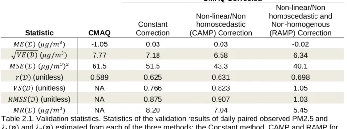
three performance evaluation methods (the last three columns of Table 2.1). The magnitude of 𝑀𝐸(𝒟) drops from −1.05 (𝜇𝑔/𝑚3) for CMAQ to 0.03 (𝜇𝑔/𝑚3) , 0.03 (𝜇𝑔/𝑚3) and −0.02 (𝜇𝑔/𝑚3) for the Constant, CAMP and RAMP methods, respectively. This was expected by design due to each method eliminating systematic errors across 𝒟. The model performance evaluation methods differ in their abilities to reduce random errors, as demonstrated by the √𝑉𝐸(𝒟) statistic. The √𝑉𝐸(𝒟) statistic progressively reduces from 7.77 (𝜇𝑔/𝑚3) for CMAQ to 7.18 (𝜇𝑔/𝑚3), 6.58 (𝜇𝑔/𝑚3) and 6.34 (𝜇𝑔/𝑚3) for the Constant, CAMP and RAMP methods, respectively. This translates in a total error that is lower for RAMP (𝑀𝑆𝐸 = 40.1 (𝜇𝑔/𝑚3)2) than for CAMP (𝑀𝑆𝐸 = 43.3 (𝜇𝑔/𝑚3)2) and the Constant method (𝑀𝑆𝐸 = 51.5(𝜇𝑔/𝑚3)2). This corresponds to a 22.1% reduction in MSE from the Constant to the RAMP method. This finding is further confirmed by the correlation between observed and 𝜆1(𝒑) values, which progressively increases from 𝑟 = 0.589 for CMAQ to 𝑟 = 0.698 for RAMP. These results demonstrate that 𝜆1(𝒑) calculated by the RAMP method is more accurate than the raw CMAQ output or the CMAQ corrected values obtained from the other model performance evaluation methods.
17
is attenuated with the CAMP method, which has an 𝑀𝑅(𝒟) equal to 70.4 𝜇𝑔/𝑚3 corresponding to a 29% overestimation compared to the RAMP estimates.
Overall these validation results demonstrate that the RAMP method provides a 𝜆1(𝒑) value that better corrects systematic errors than other performance evaluation methods and provides a 𝜆2(𝒑) value that better estimates random errors compared to other model performance evaluation methods. We hypothesize that this is due to the RAMP method being better able to assess the spatial and temporal uncertainty of systematic and random errors compared with other model performance evaluation methods.
Statistic CMAQ
CMAQ Corrected Constant Correction Non-linear/Non homoscedastic (CAMP) Correction Non-linear/Non homoscedastic and Non-homogenous (RAMP) Correction 𝑀𝐸(𝒟) (𝜇𝑔/𝑚3)
-1.05 0.03 0.03 -0.02
√𝑉𝐸(𝒟) (𝜇𝑔/𝑚3)
7.77 7.18 6.58 6.34
𝑀𝑆𝐸(𝒟) (𝜇𝑔/𝑚3)2
61.5 51.5 43.3 40.1
𝑟(𝒟) (unitless) 0.589 0.625 0.631 0.698
𝑉𝑆(𝒟) (unitless) NA 0.766 0.823 1.05
𝑅𝑀𝑆𝑆(𝒟) (unitless) NA 0.875 0.907 1.03
𝑀𝑅(𝒟) (𝜇𝑔/𝑚3) NA 8.20 7.04 5.45
Table 2.1. Validation statistics. Statistics of the validation results of daily paired observed PM2.5 and 𝜆1(𝒑) and 𝜆2(𝒑) estimated from each of the three methods: the Constant method, CAMP and RAMP for 2001 across the continental United States. The CMAQ column are the statistics between the paired observed and CMAQ concentrations. VS is variance of the standardized errors, RMSS is square root of the mean squared standardized errors and MR is the mean of the square root of 𝜆2(𝒑).
2.3.3 Stochastic Simulation Results
The RAMP estimates of 𝜆1(𝒑) and 𝜆2(𝒑) obtained for 2001 were selected as the true mean and variance, respectively, of the observed values. The CMAQ modeled output was selected as the modeled value 𝑥̃(𝒑). We obtained a stochastic realization of 𝑥̂∗(𝒑)~𝑁(𝜆
1(𝒑), 𝜆2(𝒑)) for each observed space/time location. Paired 𝑥̃(𝒑) and 𝑥̂∗(𝒑) values extracted for each observed space/time location. The Constant, CAMP and RAMP model performance evaluation methods are used to re-calculate 𝜆1∗(𝒑) and 𝜆2∗(𝒑) based only on 𝑥̃(𝒑) and 𝑥̂∗(𝒑) for 2001. The re-calculated 𝜆
1 ∗
(𝒑) and 𝜆2 ∗
18
The map of the true systematic error 𝑥̂(𝒑) − 𝜆1(𝒑) for July 1, 2001 displays by design clear geographical trends identifying well defined regions where systematic error is large. The map of re-calculated systematic error 𝑥̂(𝒑) − 𝜆1∗(𝒑) obtained using the Constant method is constant and is therefore unable to capture the spatial variability in systematic errors. The corresponding map obtained with the CAMP method is able to capture spatial variability occurring across the entire modeling domain, but unable to capture the regional and fine scale variability in systematic errors. However, the corresponding RAMP map captures spatial variability of systematic errors at a fine spatial scale. A correlation coefficient 𝑟 was calculated between 𝑥̂(𝒑) − 𝜆1(𝒑) and 𝑥̂(𝒑) − 𝜆1∗(𝒑) for July 1, 2001. This correlation coefficient was 0%, 24.0% and 76.1% for the Constant, CAMP and RAMP methods, respectively. These results demonstrate that the RAMP method is better able to capture fine scale spatial variability of systematic errors.
Similar results were found when comparing the true 𝜆2(𝒑) with 𝜆2∗(𝒑) obtained for each model performance evaluation method, again for July 1, 2001. Qualitatively, the 𝜆2∗(𝒑) map obtained with the Constant method misrepresents the true 𝜆2(𝒑) map by failing to capture any of the spatial variability in random errors and overestimating the average random error. The 𝜆2∗(𝒑) map obtained with the CAMP method is a considerable improvement by reproducing variability at a long scale distance. However, visually, the CAMP method is unable to capture fine scale variability. The 𝜆2∗(𝒑) map obtained with the RAMP method provides a good visual reproduction of the true systematic error. These results are quantitatively supported by the correlation coefficient between 𝜆2(𝒑) and 𝜆2∗(𝒑) of 0%, 5.18% and 54.5% for the Constant, CAMP and RAMP methods, respectively.
These results demonstrate that in situations where there is regional variability in model performance, the RAMP method is better able to estimate the spatial variability of systematic errors compared to the Constant and CAMP methods. This implies the RAMP method should be considered for performance evaluation in future studies wherever it is plausible for model performance to vary spatially. 2.3.4 Evidence and Implications of Non-Linear and Non-Homoscedastic Model Performance
19
simulation results. The Constant method assumes that 𝜆1− 𝑥̃𝑘 and 𝜆2 do not vary as a function of 𝑥̃𝑘. The CAMP method assumes that 𝜆1 and 𝜆2 are non-linear functions of 𝑥̃𝑘. The first evidence of non-linear and non-homoscedastic behavior comes from the validation results. The MSE reduces from 51.5 (𝜇𝑔/𝑚3)2 for the Constant method to 43.3 (𝜇𝑔/𝑚3)2 for the CAMP method, corresponding to a 16% reduction in MSE that demonstrates that model performance improves for a non-linear and non-homoscedastic model. In the stochastic simulation results, the Constant method is unable to capture the spatial variability in systematic and random errors whereas the CAMP method is able to capture domain-wide variability of these errors. Furthermore, both the validation and stochastic simulation results indicate that the Constant method significantly over predicts random errors compared to the CAMP method. Finally, the non-homoscedastic behavior in model performance is evidenced by maps of 𝜆2(𝑥̃𝑘; ℛ(𝒑)) for different values fixed 𝑥̃𝑘 values (see Appendix A), showing that at a given region ℛ(𝒑), the error variance changes substantially from one value of 𝑥̃𝑘 to another.
From these results, one should be cautious when using linear and homoscedastic model
performance evaluation methods to explore the spatial variability of model performance. This is the usual practice of current approaches in which models can be expressed as either 𝑋̃(𝒔) = 𝛽0(𝒔) + 𝛽1(𝒔)𝑋̂(𝒔) + 𝜀(𝒔) (Fuentes and Raftery, 2005) or 𝑋̂(𝒔, 𝑡) = 𝛽0(𝒔, 𝑡) + 𝛽1(𝒔, 𝑡)𝑥̃(𝒔, 𝑡) + 𝜀(𝒔, 𝑡) (Berrocal et al., 2010b). In both cases the relationship is linear and homoscedastic when assuming a constant error variance of the noise term, i.e. 𝜀(𝒔, 𝑡)~𝑁(0, 𝜎𝜖2). The linearity of these models has advantages in terms of implementation, but they fail to account for the non-linear and non-homoscedastic nature of model performance. This may undermine their capacity to fully capture spatial variability in model performance. Furthermore, these methods may overestimate the error variance. By contrast the RAMP method provides a novel alternative that fully captures the space/time variability of non-linear non-homoscedastic model performance and, as a result, provides a novel description of the spatial patterns in systematic and random errors across the spatiotemporal continuum.
2.3.5 Spatial Patterns of Systematic and Random Errors
20
what we know about CMAQ. That is, CMAQ generally struggles with estimating high values of PM2.5 (Yu et al., 2012, 2008). Areas shown with negative 𝑀𝐸(𝒑) values in Fig. 2.3 (i.e. where PM2.5 is under predicted) coincide with areas shown to have high 𝜆1(𝒑) values in Fig. 2.2d (i.e. where PM2.5 levels are high).
The RAMP analysis provides a map of 𝑀𝐸2(𝒑) across the continuous space/time domain (as opposed to being restricted to only monitoring stations). This makes it possible to clearly delineate and identify specific regions with high 𝑀𝐸2(𝒑) values and quantify their geographical extent. To illustrate this capability, we identified in Fig. 2.2a six regions (labeled 1-6) defined as having relatively high systematic error (i.e. 𝑀𝐸2(𝒑) ≥ 17.4 (𝜇𝑔/𝑚3)2). The areas of high systematic error are quantified as follows: (1) the Great Lakes (15,552 𝑘𝑚2), (2) the Appalachian Mountains (116,640 𝑘𝑚2), (3) the South East
(38,880 𝑘𝑚2), (4) Southern California (73,872 𝑘𝑚2), (5) Northern California (75,168 𝑘𝑚2) and (6) the Rocky Mountains (290,304 𝑘𝑚2).
Some of the regions identified for their high systematic errors are corroborated in the literature. The over prediction in region 1 (the Great Lakes) is in line with an overestimation of residential wood burning in the region reported in the National Emissions Inventory (NEI) (Appel et al., 2008). Region 3 (South East) includes Atlanta where PM2.5 is over estimated and an area to its South where PM2.5 is under estimated. CMAQ is known to under predict PM in the South East. Some of this under prediction may be associated with highly uncertain SOA chemistry, particularly including chemistry from biogenic emissions (Chan et al., 2010; Morris et al., 2006). Likewise high systematic error in the mountain regions 2 and 6 (Appalachia Mountains and the Rockies) can be associated with the known difficulties in
21
The map of 𝑉𝐸(𝒑) in Fig. 2.2b delineates areas with high random errors. It is interesting to note that areas of high systematic errors are always fully contained within areas of high random error as seen by comparing Fig. 2.2a and Fig. 2.2b. To our knowledge these are the first maps delineating regions of high random errors and finding general collocation with (and of about twice the magnitude of) systematic errors. If both systematic and random errors are caused by similar processes, then presumably reducing systematic errors could have the added benefit of also addressing collocated random errors.
Figure 2.3. Map of RAMP mean error. Daily PM2.5 across the continental United States on 07/01/2001 displaying 𝑀𝐸(𝒑) in 𝜇𝑔/𝑚3. The 6 regions of high random error delineated in Figure 2.2b are delineated in the dashed orange line.
2.4 Conclusions
This work introduces a spatiotemporal approach that can estimate and distinguish systematic from random error of predictions made by regulatory air quality models at any location of interest. The estimation of systematic and random error is created in a manner that does not assume that the
22
23
CHAPTER 3: INCORPORATING REGIONALIZED AIR QUALITY MODEL PERFORMANCE EVALUATION IN A NATIONWDIE GEOSTATISTICAL DATA INTEGRATION OF DAILY PM2.52 3.1 Introduction
The Clean Air Act of 1990 established regulatory standards for air pollutants in the United States (Boldo et al., 2006; Pope et al., 2009). Currently there are six “criteria air pollutants” regulated by the US Environmental Protection Agency (EPA) due to their detriment to human health and the environment, including Particulate Matter ≤ 2.5 micrometers (PM2.5). PM2.5 is associated with a host of adverse health outcomes including increased risk of cardiovascular and respiratory disease and mortality (Beelen et al., 2007; Krewski et al., 2009; Pope et al., 2004). To ensure PM2.5 does not exceed the regulatory standard, a nationwide monitoring network has been established that measures PM2.5 concentrations on a regular basis. However, despite the significant number of regulatory stations, there are large monitoring gaps that exist in many parts of the country. These can become problematic in both epidemiologic studies when attempting to predict exposures and in regulatory settings when establishing attainment. From an epidemiologic standpoint, modeled data such as Chemical Transport Models (CTMs) and satellite data can be a means to fill in the gaps left from observed data (Brauer et al., 2015; Tang et al., 2016; van Donkelaar et al., 2015). CTMs (e.g. Community Multiscale Air Quality (CMAQ) model) are deterministic and combine emissions, meteorology and chemistry to predict ambient pollution concentration across the entirety of a gridded modeling domain (Appel et al., 2013b; Foley et al., 2015a, 2015b).
In air quality modeling there has been a recent surge in data fusion methods. These methods combine different air quality sources together, in particular, observed data with gridded modeled data (Berrocal et al., 2010a; Crooks and Isakov, 2013; Fuentes and Raftery, 2005). Many studies that combine data sources focus on epidemiologic studies with the goal of having accurate exposure prediction that reduce misclassification (Beckerman et al., 2013). Observed data are considered highly accurate and
2This chapter was submitted as an article to the journal Environmental Science and Technology. Reyes,
produce low prediction errors but are potentially sparsely measured. Corresponding prediction methods which may only use observed data (e.g. kriging) have lower spatial refinement. CMAQ data are
considered less accurate than observed data but have excellent spatial and temporal coverage along with a higher level of spatial refinement.
Previous popular data fusion methods include the Downscaler method and Bayesian Melding (Berrocal et al., 2012, 2010a, 2010b). The Downscaler method takes output of a CTM model and uses it as an independent variable in the Downscaler regression model. The Bayesian Melding approach
characterizes the full uncertainty in observed, modeled and the true underlying process of the air pollutant of interest. However, this method is computationally intensive and has only been applied in a spatial setting. Inherent in both of these methods are assumptions of linearity and homoscedastic behavior in the model.
This work proposes the Regionalized Air quality Model Performance (RAMP) incorporation into the Bayesian Maximum Entropy (BME) geostatistical framework (Reyes et al., 2016; Xu et al., 2016). BME is an extension of linear kriging and has the flexibility of incorporating multiple data sources together. The RAMP BME data fusion method is an extension of the Constant Air quality Model
Performance (CAMP) method introduced by de Nazelle et al. (de Nazelle et al., 2010). The novel RAMP approach to model performance evaluation is able to quantify model performance metrics across the entirety of a domain and fully characterizes model performance at each space/time grid location over the fully spectrum of given modeled values. This proposed data fusion method can capture the accuracy of observed data with the spatial refinement of CMAQ data without assumptions of linearity and
homoscedastic behavior.
A demonstration of the BME data fusion method developed in this work combines CMAQ modeled data with observed data to predict daily PM2.5 mass across the continental US for 2001. The BME method takes advantage of low prediction error associated with observed data along with the high spatial refinement associated with CMAQ modeled data. Results are then compared to a frequentist version of the Downscaler method. These results improve the spatial refinement of PM2.5 predictions and offer a more realistic exposure profile which can be used in epidemiologic analysis to reduce
25
misclassification and more clearly uncover the true association between participants’ air pollution exposures and health outcomes.
3.2 Materials and Methods
3.2.1 Observed and modeled data
The daily observed PM2.5 concentration for each monitoring site/day during 2000-2002 were constructed based on raw monitoring data from monitoring stations measuring either hourly or daily PM2.5 concentrations obtained from the EPA’s Air Quality Systems data base (US EPA, n.d.). Daily concentrations for PM2.5 were also constructed from hourly modeled data averaged to daily for years 2001 and 2002 using CMAQv4.5 across the contiguous United States on a 36 km grid. For more detailed information regarding the aggregation and pairing process of observed and modeled data see Appendix A.
3.2.2 BME estimation methodology
BME is a mathematically rigorous geostatistical space/time framework originally developed in a geostatistical setting by Christakos (Christakos, 2000; Christakos et al., 2001). BME can incorporate information from multiple data sources and is implemented using the BMElib suite of functions in
26
In this study we use an S/TRF to describe the variability of daily PM2.5 mass across the US in 2001. Our notation for an S/TRF will consist of denoting a single random variable 𝑍 in capital letters, its realization, 𝑧, in lower case and vectors and matrices in bold faces (e.g. 𝒁 = [𝑍1, … , 𝑍𝑛]𝑇 and 𝒛 = [𝑧1, … , 𝑧𝑛]𝑇). Let 𝑍(𝒑) = 𝑍(𝒔, 𝑡) be a Space/Time Random Field (S/TRF) representing daily PM2.5. The BME data fusion method incorporates both modeled and observed data. Let 𝑍̂(𝒑) be the random variable representing the observed concentration, 𝑧̂(𝒑) be its known (i.e. observed) value and 𝑧̃(𝒑) be the CMAQ modeled value at location 𝒑.
We define the transformation of observed PM2.5 data 𝒛ℎ observed at locations 𝒑ℎ as
𝒙ℎ= 𝒛ℎ– 𝑜𝑍(𝒑ℎ) (Equ. 3-2)
where 𝑜𝑍(𝒑) may be any deterministic offset that can be mathematically calculated without error as a function of the space/time coordinate 𝒑. We then define 𝑋(𝒑) as a homogeneous/stationary S/TRF representing the variability and uncertainty associated with the transformed data 𝒙ℎ, and we let 𝑍(𝒑) = 𝑋(𝒑) + 𝑜𝑍(𝒑) be the S/TRF representing PM2.5. We can then calculate 𝑧̈𝑘, the predicted daily PM2.5 at unmonitored location 𝒑𝑘, by obtaining the BME estimate 𝑥̈𝑘 for the transformed S/TRF 𝑋(𝒑) at the estimation point 𝒑𝑘 and adding 𝑜𝑧(𝒑𝑘), the offset calculated at 𝒑𝑘. In this work we calculate the offset using a space/time composite kernel smoothing of the data (Lee et al., 2012). The covariance model for the homogeneous/stationary S/TRF 𝑋(𝒑) is developed from the experimental covariance of the
transformed data 𝒙ℎ = 𝒛ℎ– 𝑜𝑍(𝒑ℎ). The offset and the corresponding covariance in this work are chosen as having the best combination of low variance and the high autocorrelation. For detailed information regarding the calculation of the offset function and covariance model, see Appendix B.
3.2.3 Regionalized Air quality Model Performance (RAMP) soft data construction
27
given estimation location, several hard and soft data go into the corresponding prediction. Thus, we can further expand 𝑓𝑆(𝒙𝒔) to the following expression:
𝑓𝑆(𝒙𝒔) = ∏ 𝑓(𝑥𝑖|𝑥̃𝑖, 𝒑𝑖) 𝑛𝑚
𝑖 , (Equ. 3-3)
where 𝑛𝑚 is the number of CMAQ grids used in the calculation of the soft data, 𝑓(𝑥𝑖|𝑥̃𝑖, 𝒑𝑖) is the soft data PDF of PM2.5 concentration at the modeled data location 𝒑𝑖 and 𝑥̃𝑖 is the modeled value of PM2.5 concentration after removing the offset.
For the sake of clarity of the soft data development, consider the non-transformed random variable 𝑍. The soft PDF 𝑓(𝑧𝑖|𝑧̃𝑖, 𝒑𝑖) is Gaussian distributed with mean 𝜆1 and variance 𝜆2, denoted: 𝑓(𝑧𝑖|𝑧̃𝑖, 𝒑𝑖) = Φ(𝑧𝑖; 𝜆1(𝒑), 𝜆2(𝒑)) (Equ. 3-4) The parameters 𝜆1 and 𝜆2 are dependent on the modeled value concentration around 𝒑. The parameters 𝜆1 and 𝜆2 are estimated using the equations given below:(de Nazelle et al., 2010)
𝜆1(𝑧̃𝑘; ℛ(𝒑)) = 𝑀[𝑍̂|𝑧̃𝑘; ℛ(𝒑)] ≈ 1
𝑛(𝑧̃𝑘;ℛ(𝒑))∑ 𝑧̂𝑖 (Equ. 3-5) 𝜆2(𝑧̃𝑘, ℛ(𝒑)) = 𝑉[𝑍̂|𝑧̃𝑘; ℛ(𝒑)] ≈ 1
𝑛(𝑧̃𝑘;ℛ(𝒑))−1∑(𝑧̂𝑖− 𝜆1(𝑧̃𝑘; ℛ(𝒑)))
2
(Equ. 3-6)
where 𝑛(𝑧̃𝑘; ℛ(𝒑)) is the number of paired modeled and observed points within region ℛ(𝒑)associated with space/time location 𝒑 which are from the 3 closest monitoring stations within 180 days around 𝑧̃𝑘. Stated simply, 𝜆1 is estimated through pooling all paired modeled and observed data together in region ℛ(𝒑)associated with space/time location 𝒑 and close to the modeled value 𝑧̃𝑘. The mean of all the near-by observed data are taken to calculate 𝜆1(𝑧̃𝑘; ℛ(𝒑)). Similarly, the variance of all the near-by observed data are taken to calculate 𝜆2(𝑧̃𝑘, ℛ(𝒑)). Modeled and observed data are paired if an observed datum lies within a given grid.
Although 𝜆1(𝑧̃𝑘; ℛ(𝒑)) and 𝜆2(𝑧̃𝑘, ℛ(𝒑)) can be calculated for any arbitrary 𝑧̃𝑘, in this work we set 𝑧̃𝑘= 𝑧̃(𝒑), where 𝑧̃(𝒑) is the CMAQ modeled value at 𝒑. By replacing 𝑧̃𝑘 with 𝑧̃(𝒑) in Equ. 5 and Equ. 3-6, we define 𝜆1(𝑧̃(𝒑), ℛ(𝒑)) = 𝜆1(𝒑) and 𝜆2(𝑧̃(𝒑), ℛ(𝒑)) = 𝜆2(𝒑). For the sake of shorthand in this work, we further define 𝜆1= 𝜆1(𝒑) and 𝜆2= 𝜆2(𝒑).
3.2.4 Leave One Out Cross Validation (LOOCV) accuracy analysis
28
BME for each removed datum (without recalculating the offset or the covariance model) using all the data from the remaining monitoring stations and soft data. This is repeated again for each monitoring station. However, instead of only removing data from a single monitoring station, all observed data within a given radius from the monitoring station (100 km, 200 km, 300 km, … , 900 km) are removed.
The difference between each prediction value 𝑧̈𝑖 and observed value 𝑧̂𝑖 is the prediction error, 𝑒𝑖= 𝑧̈𝑖− 𝑧̂𝑖. The prediction accuracy is quantified based on statistics of prediction errors, which consist of the Mean Squared Error (MSE, (𝜇𝑔/𝑚3)2), Mean Error (ME, 𝜇𝑔/𝑚3) and the Pearson’s correlation coefficient (𝑟, unitless) between observed and predicted values. BME data fusion predictions are then compared to kriging (i.e. predictions created only using observed data).
Because 𝜆1 and 𝜆2 are written in terms of an expected value and variance, respectively,
performance metrics can be written in terms of these quantities. Namely, mean error and variance of error for an arbitrary 𝒑 (see Chapter 2).
𝜆1(𝒑) = 𝑧̃(𝒑) − 𝑀𝐸(𝒑) (Equ. 3-7)
𝜆2(𝒑) = 𝑉𝐸(𝒑) (Equ. 3-8) Using the relation equating mean squared error to mean error and variance of error (i.e. 𝑀𝑆𝐸 = 𝑀𝐸2+ 𝑉𝐸), LOOCV results can be stratified by the scaled mean error statistic,
𝑆𝑀𝐸(𝒑) = 𝑀𝐸2(𝒑)/𝑀𝑆𝐸(𝒑). (Equ. 3-9) 3.2.5 Comparison to the frequentist Downscaler method
This work is compared to a frequentist implementation of the space/time Downscaler method (Berrocal et al., 2010a). A full description of this method can be found in Appendix B. In short, 𝑍(𝒑)~𝑁(𝜇𝑍, 𝑐𝑍) where 𝑍(𝒑) is the pollutant of interest. 𝑍̂(𝒑) is defined as:
𝑍̂(𝒑) = 𝛽0𝑡+ 𝛽0(𝒑) + 𝛽1𝑡𝑧̃(𝒑) + 𝛽1(𝒑)𝑧̃(𝒑) + 𝜖(𝒑), (Equ. 3-10) where 𝛽0𝑡 is the constant additive bias, 𝛽0(𝒑) is the additive bias that changes as a function of 𝒑, 𝛽1𝑡 is the constant multiplicative bias, 𝛽1(𝒑) is the multiplicative bias that changes as a function of 𝒑, 𝑧̃(𝒑) is the modeled value concentration of 𝒑 and 𝜖(𝒑) is random noise. In the space/time application of the
29
which both the additive and multiplicative bias are treated independently across time. The results given below are a frequentist implementation of this method (i.e. all parameters are estimated empirically). 3.3 Results and Discussion
3.3.1 PM2.5 data fusion demonstration of RAMP BME
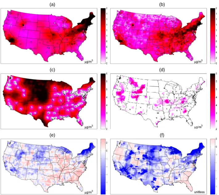
A demonstration of the BME data fusion method was completed by combining daily observed PM2.5 with daily systematic error corrected CMAQ predictions were generated using CMAQv4.5 on a 36 km grid across the continental United States for 2001. BME predictions were created at the centroid of each CMAQ grid. Results of the BME data fusion method and kriging are displayed across the continental US on 07/01/2001 (Fig. 3.1). There is a clear spatial pattern for BME across the day as shown through the posterior mean (Fig. 3.1b). There is an area of high daily PM2.5 predictions (over 20 𝜇𝑔/𝑚3) in Southern California, which is an area known to have high PM2.5 concentrations (Fann et al., 2012). There is a distinctive band of high concentrations, also around 20 𝜇𝑔/𝑚3, in the Eastern US extending from the New England area to West Virginia ending around Illinois. Areas of low concentrations (between 0 − 4 𝜇𝑔/𝑚3) can mostly be found in the US states bordering Canada including Montana, North Dakota and Minnesota, which are states known to have relatively low concentrations of daily PM2.5 (Fann et al., 2012). For comparison to the BME data fusion method, kriging predictions are created for the same locations across the US on 07/01/2001 using only observed daily PM2.5 data (Fig. 3.1a,c). Generally speaking, the overarching spatial patterns of the kriging map are similar to those of BME (Fig. 3.1a). Kriging mean predictions show a PM2.5 plume encompassing a larger area over Southern California compared to BME. Likewise, the kriging map depicts the entirety of New England as having large PM2.5 concentrations. The pattern of relatively high PM2.5 concentration continues across West Virginia and Illinois, albeit at lower concentrations than are predicted for BME. For kriging, areas of the country showing the lowest concentration are the same border states. However, the lowest concentrations of PM2.5 for kriging are between 4 − 8 𝜇𝑔/𝑚3, while low concentrations for BME are between 1 − 5 𝜇𝑔/𝑚3.
The uncertainty with both the BME and kriging mean estimates is quantified by their
30
around areas that are far from observed data. This is in stark contrast with the BME standard deviation map, which displays substantially lower standard deviations in the same areas. By design the BME framework benefits from information provided by observations as well as CMAQ data, where the latter covers the entirety of the mapping domain. It is the addition of these CMAQ data that are responsible for the sizable decrease in the standard deviation in areas suffering from sparse air quality monitoring. As a result, the average estimation error standard deviation across the US drops substantially from kriging to BME. The average standard deviation on 07/01/2001 is 5.6 𝜇𝑔/𝑚3 for kriging while that value drops to 2.0 𝜇𝑔/𝑚3 for BME, indicating a more than two fold decrease in mapping uncertainty across the US.
31
(a) (b)
(c) (d)
(e) (f)
Figure 3.1. Map of kriging and BME mean and variance. Daily PM2.5 across the continental United States on 07/01/2001 displaying the (a) kriging mean estimate (𝐸𝐾𝑟𝑖𝑔[𝒁]), (b) BME mean estimate (𝐸𝐵𝑀𝐸[𝒁]), (c) kriging standard deviation, (d) BME standard deviation, (e) 𝐸𝐵𝑀𝐸[𝒁] − 𝐸𝐾𝑟𝑖𝑔[𝒁] and (f) (𝜆1− 𝐸𝐾𝑟𝑖𝑔[𝒁])/ √𝜆2. Plots. (a)-(e) are in 𝜇𝑔/𝑚3 and (f) is unitless.
3.3.2 Validation results
32
radii, and that this outperformance enhances significantly with increasing cross validation radii. As increasing distance between the prediction location and the nearest observed data increases, the kriging method suffers a significant increase in MSE, which is tampered for BME due to the information
contributed by the CTM data.
Because all observations can be paired with a corresponding CMAQ value, all observed data can be paired with the corresponding error corrected CMAQ value 𝜆1 characterizing the expected PM2.5 concentration at that location. Hence the PCMSE can further be explored as a function of different selection criteria for 𝜆1. The criteria used in Fig. 3.2a correspond to the baseline case (all observations are included), 𝜆1≥ 12.4 𝜇𝑔/𝑚3 and 𝜆1≥ 16.8 𝜇𝑔/𝑚3. The PCMSE becomes more negative as 𝜆1 increases, and this becomes even more pronounced for larger cross validation radii.
Likewise the CMAQ value collocated with each observation can be characterized by the model performance parameter 𝑆𝑀𝐸(𝒑) at the CMAQ grid coordinate 𝒑, which quantifies the proportion of systematic to total error for the CMAQ prediction.(Reyes et al., 2016) When the PCMSE is calculated using only observations for which the collocated CMAQ values are such that 𝑆𝑀𝐸(𝒑) ≥ 22%, the reduction in MSE from kriging to BME is even more pronounced (Fig. 3.2b). The PCMSE ranges from −3.1% to −32% depending on 𝜆1 and cross validation radii. The PCMSE falls more quickly for increasing radii as the 𝑆𝑀𝐸(𝒑) ≥ 22% criteria is added, especially for radii 200-400 km. For the baseline case, previous to the application of the proportional systematic error criteria, the PCMSE is −2.1% for 200 km, −4.2% for 300 km and −9.6% for 400 km. After the proportional systematic error criterion is applied the PCMSE is −10% for 200 km, −12% for 300 km and −16% for 400 km.
33 (a)
(b)
(c)