P-TYPE POINT CONTACT GERMANIUM DETECTORS AND THEIR APPLICATION IN RARE-EVENT SEARCHES
Graham Kurt Giovanetti
A dissertation submitted to the faculty at the University of North Carolina at Chapel Hill in partial fulfillment of the requirements for the degree of Doctor of Philosophy in the
Department of Physics.
Chapel Hill 2015
c 2015
ABSTRACT
Graham Kurt Giovanetti: P-type Point Contact Germanium Detectors and Their Application in Rare-Event Searches
(Under the direction of John F. Wilkerson)
In the last two decades, experimental results from the direct detection of solar, reactor, and atmospheric neutrinos have provided convincing evidence that neutrinos have mass, the first definitive evidence of physics beyond the Standard Model. The existence of massive neutrinos opens many questions about the neutrino’s intrinsic properties, including the ab-solute mass, the relative hierarchy of the neutrino mass states, and the Majorana or Dirac nature of the neutrino. The Majorana Demonstrator is an array of p-type point con-tact (PPC) high purity germanium detectors that will search for the neutrinoless double-beta decay (0νββ) of 76Ge, a process that can only occur if the neutrino is a Majorana particle.
PPC detectors have several characteristics that make them well suited for a 76Ge 0νββ
search, including sub-keV energy thresholds that allow for background rejection based on low-energy x-ray tagging. This feature makes theMajorana Demonstratorsensitive to signals that might be present from processes that are not in the current Standard Model of particle physics.
ACKNOWLEDGEMENTS
I would like to thank John Wilkerson for his support, mentorship, and for providing a careful balance of guidance and freedom throughout my graduate career. I would also like to thank Reyco Henning for his mentorship and advice. I have had the pleasure of working with and learning from many great scientists. Thanks to Jason Detwiler, Steve Elliott, Kevin Gio-vanetti, Matt Green, Mark Howe, Mike Marino, Chris O’Shaughnessy, David Radford, Alexis Schubert, and all of my other Majorana and UNC ENAP collaborators. A special thank you to Paddy Finnerty who was the driving force behind MALBEK and a constant source of useful discussion and welcome distraction. Thank you to Sean Finch, Derek Roundtree, Werner Tornow, Lhoist North America, Matthew Busch, and the rest of the TUNL technical staff for their logistical support and help with MALBEK operations. Finally, thanks to my parents for the gift of education, my family and friends for their unwavering support, and Catherine for keeping it all fun.
TABLE OF CONTENTS
LIST OF TABLES . . . ix
LIST OF FIGURES . . . x
LIST OF ABBREVIATIONS AND SYMBOLS . . . xiii
1 Introduction . . . 1
1.1 Neutrinoless Double-beta Decay . . . 1
1.2 The MAJORANA DEMONSTRATOR . . . 4
1.3 Direct WIMP Detection . . . 8
1.4 Outline of This Dissertation . . . 10
2 The MAJORANA Low-background BEGe Detector at KURF . . . 12
2.1 Detector and Shielding . . . 12
2.2 Data Acquisition System and Slow Controls . . . 14
2.2.1 Digitizer Configuration . . . 17
2.3 MALBEK Operation History . . . 20
2.4 Data Processing . . . 21
2.4.1 Energy Calculation and Calibration . . . 22
2.4.2 Data Selection Cuts . . . 23
3.1 Signal Formation in PPC Detectors . . . 25
3.2 Surface Events in PPC Detectors . . . 28
3.3 Surface Event Identification . . . 30
3.3.1 t10−90 Rise-time . . . 32
3.3.2 wpar . . . 36
3.4 Surface Event Removal . . . 40
3.4.1 Surface Event Distributions From Varying Sources . . . 40
3.4.2 Fast Event Survival as a Function of Cut Position . . . 47
3.4.3 Attenuated Waveform Study . . . 50
3.4.4 Defining a Surface Event Cut . . . 54
3.5 Conclusions . . . 56
4 Surface Event Modeling . . . 58
4.1 Surface Event Signal Formation Model . . . 58
4.1.1 Basic Simulation . . . 60
4.1.2 Simulation with Lithium Precipitates . . . 61
4.2 Properties of the Model . . . 63
4.3 Comparison of Simulation Results to Data . . . 66
4.4 Conclusion . . . 72
5 Rare-Event Searches with MALBEK . . . 75
5.1 The 89.5 kg-d Dataset . . . 75
5.1.1 Overview of Data Processing . . . 76
5.1.3 Systematic Effects . . . 80
5.2 Search for Weakly Interacting Massive Particles . . . 85
5.2.1 Expected Signal . . . 85
5.2.2 Statistical Method . . . 89
5.2.3 Model and Fit Results . . . 91
5.3 Search for Solar Axions . . . 101
5.3.1 Expected Signal . . . 103
5.3.2 Results . . . 104
5.4 Search for Pauli Exclusion Principle Violating Decays . . . 110
5.4.1 Expected Signal . . . 112
5.4.2 Model and Fit Results . . . 112
6 Conclusions . . . 117
6.1 Summary of Results . . . 117
6.2 Extensions . . . 118
6.3 Outlook . . . 119
LIST OF TABLES
2.1 Peaks used for energy calibration . . . 22
5.1 Peaks in the 89.5 kg-d spectrum . . . 78
5.2 Summary of systematic errors . . . 84
5.3 Parameters fit during the WIMP analysis . . . 95
5.4 Parameters fit during the solar axion analysis . . . 106
LIST OF FIGURES
1.1 Majorana Demonstrator cryostat drawing . . . 5
1.2 Majorana Demonstrator shield drawing . . . 6
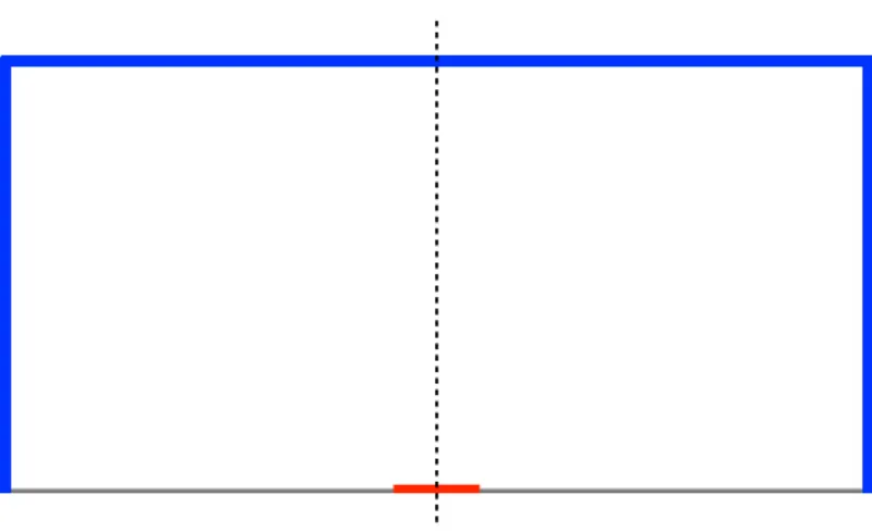
1.3 Schematic of a PPC detector . . . 7
2.1 MALBEK shield drawing . . . 14
2.2 MALBEK data acquisition system block diagram . . . 15
2.3 Trigger efficiency of the SIS3302 . . . 18
2.4 Basic data selection cut efficiencies . . . 24
3.1 Weighting potential within a PPC detector . . . 26
3.2 Multi-site and single-site events in a PPC detector . . . 27
3.3 Comparison of energy spectra with and without lead shims . . . 29
3.4 Expected signal from a 15 GeV WIMP . . . 30
3.5 Charge collection times calculated from a 2D diffusion model . . . 31
3.6 Waveforms from a bulk event and a surface event . . . 32
3.7 Comparison of two t10−90 rise-time calculation techniques . . . 33
3.8 Example of a failed t10−90 rise-time calculation . . . 34
3.9 t10−90 distribution for pulser generated data . . . 35
3.10 Block diagram of a discrete stationary wavelet transformation . . . 36
3.11 Example wpar calculation . . . 37
3.12 wpar versus energy distribution for fast pulser generated data . . . 38
3.13 wpar versus energy distribution for slow pulser generated data . . . 38
3.14 Correlation between wpar and t10−90 . . . 39
3.15 wpar versus energy distributions for data with and without lead shims . . . . 42
3.16 wpar versus energy distribution for 241Am source data . . . 43
3.17 wpar versus energy distribution for the 89.5 kg-d shielded exposure . . . 44
3.19 89.5 kg-d spectrum after removing events with wpar values less than 15 . . . 48
3.20 Counts remaining as a function of wpar cut in the 241Am source dataset . . . 49
3.21 Counts remaining as a function of wpar cut in the lead source dataset . . . . 50
3.22 Counts remaining as a function of wpar in the 89.5 kg-d dataset . . . 51
3.23 wpar versus energy distribution for high energy shielded MALBEK data . . 51
3.24 wpar versus energy distribution for attenuated data . . . 52
3.25 wpar distributions for attenuated data in two energy regions . . . 53
3.26 Counts remaining as a function of wpar cut in the attenuated dataset . . . . 54
3.27 89.5 kg-d data before and after wpar cut . . . 56
4.1 Calculated lithium concentration in a lithium drifted n+ contact . . . . 59
4.2 Results from a simple surface event model . . . 61
4.3 Example simulated lithium distribution . . . 62
4.4 Surface event model simulation results . . . 63
4.5 Simulation results with varying precipitate size . . . 64
4.6 Simulation results with varying precipitate density . . . 65
4.7 Simulation results with varying precipitate distributions . . . 66
4.8 Simulation results with varying lithium layer depths . . . 67
4.9 Rise-time distribution for 241Am data . . . . 68
4.10 Rise-time distribution for 109Cd data . . . 68
4.11 Simulated 241Am rise-time distribution compared to data . . . 70
4.12 Simulated 241Am energy spectrum compared to data . . . 71
4.13 Simulated 109Cd rise-time distribution compared to data . . . 72
4.14 Simulated 109Cd energy spectrum compared to data . . . 73
5.1 89.5 kg-d spectrum after all cuts . . . 77
5.2 Counts in the 68,71Ge K-shell capture peak over time. . . 79
5.4 Widths of peaks in the low energy region . . . 92
5.5 8.0 GeV WIMP fit at 90% C.L. . . 94
5.6 λ(σnuc) for an 8.0 GeV WIMP . . . 95
5.7 Number of events in the flat background versus WIMP mass . . . 96
5.8 Number of events in the L line capture peaks versus WIMP mass . . . 97
5.9 Number of background and signal events versus WIMP mass . . . 97
5.10 90% C.L. WIMP exclusion curves with varying quenching factors . . . 99
5.11 90% C.L. WIMP exclusion limit . . . 100
5.12 Axio-electric cross section of germanium . . . 104
5.13 Calculated solar axion flux . . . 105
5.14 λ(Nsignal) for a sub-keV solar axion . . . 107
5.15 Solar axion fit at 90% C.L. . . 108
5.16 Axio-electric coupling exclusion curves . . . 110
5.17 λ(PEP transitions) with and without systematic errors . . . 115
LIST OF ABBREVIATIONS AND SYMBOLS
0νββ Neutrinoless Double-beta Decay 2νββ Double-beta Decay
BEGe Broad Energy Germanium C.L. Confidence Level
CMB Cosmic Microwave Background
DFSZ Dine, Fischler, Srednicki, and Zhitnitsky Axion Model DSWT Discrete Stationary Wavelet Transform
DWT Discrete Wavelet Transform GAT Germanium Analysis Toolkit HPGe High Purity Germanium
KSVZ Kim, Shifman, Vainstein, and Zakharov Axion Model KURF Kimballton Underground Research Facility
MALBEK MajoranaLow-background BEGe Detector at Kimballton PEP Pauli Exclusion Principle
PPC P-type Point Contact
Q End-point Energy
ROI Region of Interest SBC Single Board Computer
SIS3302 Struck Innovativ Systeme 3302 Digitizer SURF Sanford Underground Research Laboratory WIMP Weakly Interacting Massive Particle
CHAPTER 1: Introduction
Section 1.1: Neutrinoless Double-beta Decay
Physicists have observed the flavor oscillation of neutrinos from a variety of sources [1], showing in all cases that the neutrino flavor states (νe, νµ, ντ) are distinct from the neutrino
mass states (ν1, ν2, ν3) and can be written as
να =
X
i
Uαiνi (1.1)
whereα=e, µ, τ;i= 1,2,3; and Uαi is the neutrino mixing matrix. Oscillation experiments
have also demonstrated that the mass splitting between the first and second neutrino mass states is much smaller than the mass splitting to the third mass state,
∆m2sol =m22−m21 ∆m2atm=|m23−(m12 +m22)/2| (1.2)
where ∆m2
sol is determined by measuring solar neutrino oscillation (νe→νµ, ντ) and reactor
neutrino oscillation ( ¯νe → ν¯µ,ν¯τ), and ∆m2atm is determined by observing atmospheric and
accelerator neutrino disappearance (νµ →ντ). While the relative mass splittings are known,
oscillation experiments are only sensitive to the absolute value of ∆m2
atm, leaving two possible
neutrino mass hierarchy scenarios. In the normal hierarchy, named for its similarity to the mass hierarchies in the quark and charged lepton sector, ν3 is the heaviest mass state. In
the inverted hierarchy, ν3 is lighter thanν1 and ν2.
in the tritium beta-decay spectrum around the 18.6 keV endpoint energy. Additional con-straints on the sum of the neutrino masses come from indirect cosmological probes. An analysis of the anisotropies of the cosmic microwave background (CMB) using five years of Wilkinson Microwave Anisotropy Probe (WMAP) data limits the sum of the neutrino masses, P
mν <1.3 eV [3]. A 2013 measurement by the PLANCK collaboration combined
with other probes of the matter distribution of the Universe results in even more stringent constraints,P
mν <0.23 eV [4]. KATRIN, the next generation direct neutrino mass tritium
beta-decay spectrometer aims to improve sensitivity of the Mainz experiment by one order of magnitude [5].
Neither oscillation experiments nor direct neutrino mass measurements provide insight into the neutrino mass generation mechanism or the neutrino’s Majorana nature. The neu-trino interacts via the weak force, which only couples to the negative chirality component of a fermion field. In the limit of a massless particle, chirality is indistinguishable from helicity. In the case of a massless neutrino, this implies that any right(left)-handed (anti-)neutrino would be sterile and unobservable, regardless of the Majorana or Dirac nature of the particle. The Standard Model therefore includes only a left(right)-handed (anti-)neutrino. With the introduction of neutrino mass, the negative chirality state (νl) becomes a superposition of
±1
2 helicity states, where the contribution from the + 1
2 helicity state is heavily suppressed by
a factor proportional to mν
E , where E is the neutrino energy. In this case, neutrino mass can
conservation and couples neutrinos to anti-neutrinos. The addition of a Majorana mass term is forbidden for charged particles because it violates charge conservation but could be allowed for electrically neutral neutrinos. The only practical way to determine whether the neutrino is a Majorana particle is by observation of neutrinoless double-beta decay (0νββ) [7].
For some even-even nuclei, the single-beta decay channel is either energetically forbidden, due to pairing forces, or heavily suppressed, e.g. 48Ca → 48Ti. In these cases, the nucleus
can double-beta decay (2νββ), simultaneously converting two neutrons into two protons and emitting two β particles and two anti-neutrinos. This process was originally suggested in 1935 by Maria Goeppert-Mayer, who estimated a lifetime for the process of approximately 1017years [8]. It wasn’t until 1987 that the first laboratory observation of 2νββwas made by
Elliott, Hahn, and Moe in82Se [9]. Physicists are now searching for neutrinoless double-beta
decay (0νββ), a related process postulated in 1939 by Wendell H. Furry [10]. In 0νββ, two neutrons are converted to two protons with the emission of twoβ particles and no neutrinos. In the simplest case of light neutrino exchange, the inverse half-life of 0νββ can be written as
1
T10/ν2 =G0ν(Qββ, Z)|M0ν|
2hm
ββi2, (1.3)
where G0ν(Qββ, Z) is a calculable phase space factor, M0ν is a nuclear matrix element, and
hmββi is the effective Majorana neutrino mass. Observation of 0νββ would indicate that
the neutrino is a Majorana particle, show that lepton number is not conserved, and give a measure of the effective Majorana neutrino mass.
The signature for 0νββ is the emission of two electrons whose summed energy is equal to the double-beta decay end-point energy (Qββ). If the effective Majorana neutrino mass
is of the order ∆2
atm, the expected 0νββ event rate from a tonne of isotope is approximately
low-background materials.
There are several experimental aspects that must be considered when building a 0νββ experiment, both when selecting the source isotope and defining the detection technique. First, the source isotope should be readily attainable, either due to its high natural abun-dance or through an established enrichment process, so that the detector mass can be made large without prohibitive cost. Selecting an isotope with a higher Qββ value has the added
benefit of moving the 0νββ ROI above the majority of backgrounds from the U and Th decay chains and providing a larger phase space for the decay. Second, the detector itself should have good energy resolution in the ROI, which maximizes the signal to background ratio. Additional background reduction can be accomplished if the detector allows event reconstruction, has good timing resolution, or can tag the daughter nucleus from the de-cay. Lastly, the detector must be constructed of radio-pure components and installed in a low-background environment. This means that the detector must be built underground, at a depth sufficient to limit high-energy muon induced neutrons and cosmogenically induced backgrounds in the detector components. The detector must also be installed in a shield that will minimize the environmental and anthropogenic backgrounds present underground, such as fast neutrons from (α, n) reactions in the surrounding rock, gammas from local sources, and radon. The detector components themselves must also be constructed from materials with low levels of primordial contaminants and limited cosmogenic activation.
Section 1.2: The MAJORANA DEMONSTRATOR
The Majorana collaboration is currently building the Majorana Demonstrator, a 40 kg array of high purity germanium (HPGe) detectors. Approximately 30 kg of these detectors are constructed from material enriched to 87% in76Ge, allowing the
Figure 1.1: Drawing of a Majorana Demonstrator cryostat. Strings of germanium crystals (turquoise) hang from the cryostat cold plate.
are stacked vertically to build detector strings that are deployed in a vacuum cryostat as shown in Figure 1.1. The strings create a thermal path from the cryostat cold plate to the germanium crystals, which must be kept at cryogenic temperatures during operation. Two cryostats, each containing 20 kg of detectors, are under construction in a cleanroom facility at the 4850’ level of the Sanford Underground Research Facility (SURF) in Lead, SD. Once complete, these cryostats will be installed in a compact shield made from electro-formed copper, commercial high purity copper, lead, plastic, and an active muon veto. The Demonstrator shield is shown in Figure 1.2. The background goal for the Demonstra-tor is 3 background counts/tonne/year in the 4 keV wide ROI around the 2039 keV 76Ge endpoint energy. This scales to a rate of 1 count/tonne/year for a Demonstrator-style tonne-scale experiment, the required background level for sensitivity to 0νββ if neutrinos follow the inverted mass hierarchy. The projected background rate for the Demonstra-tor based on radio-assay of the cryostat and shield components is less than or equal to 3.1 counts/tonne/year.
Figure 1.2: Cutaway of the Majorana Demonstrator shield. The shield is constructed of electroformed copper, commercial high-purity copper, lead, and plastic and houses two cryostats containing strings of germanium detectors.
be able to distinguish the neutrinoless double-beta decay signal, which is a localized, ef-fectively single-site event, from background multi-site events, e.g. events from gamma-rays Compton scattering multiple times within a single HPGe detector. Initially, segmented N-type coaxial detectors were considered for use in theDemonstratordue to their ability to tag events occurring across multiple segments. However, these detectors are difficult to man-ufacture and handle and, because each segment requires its own readout channel, increase the amount of potentially radio-impure material inside the cryostat.
Figure 1.3: Cross-sectional drawing of a PPC detector. The detector is axially symmetric about the dashed line. The n+ contact is shown in blue and the p+ point contact is shown in red. Bias voltage is applied to the n+ contact and signals are read out from the p+ contact.
PPC detectors typically have a diameter around 60 mm and heights ranging from 30 to 50 mm.
have a capacitance on the order of 1 pF and can be operated with sub-keV energy thresh-olds [14]. This can be used to reduce 0νββbackgrounds from cosmogenically produced 68Ge
using a time correlated analysis cut. Long lived 68Ge (Qec = 106 keV, T1/2 = 270.8 days)
decays via electron capture to68Ga (Qec = 2921.1 keV, T1/2 = 67.7 min) and can contribute
background events in the 0νββ ROI. This rate can be reduced by up to 98% by tagging L-shell capture (1.3 keV) and K-shell capture (10.3 keV) events that occur during the 68Ge
decay and vetoing for several68Ga half-lives. Finally, PPC detectors are simpler to fabricate
than segmented detectors and only require one set of readout electronics per detector, reduc-ing the amount of material within the detector cryostat. For these reasons, theMajorana collaboration is using PPC detectors in the Demonstrator.
Section 1.3: Direct WIMP Detection
Astronomical observations of galactic rotation curves, strong lensing, and the anisotropy of the CMB all suggest that visible matter only accounts for a fraction of the total mass of the Universe [1]. The missing mass can be attributed to gravitationally interacting but non-luminous dark matter that formed shortly after the Big Bang and coalesced into halos around galaxies as the Universe cooled. While dark matter has not been directly detected, a recent measurement by the Planck satellite predicts that it constitutes 26.8% of the energy density in the Universe [4]. A viable particle candidate for dark matter must be stable over the lifetime of the Universe, electrically neutral, non-relativistic and, to explain the anisotropy of the CMB, non-baryonic.
Weakly interacting massive particles (WIMPs) are a class of dark matter particle can-didates that only interact gravitationally and through the weak force and are projected to have masses between 1 and 1000 GeV. WIMP-like particles are predicted in many exten-sions of the Standard Model, including supersymmetric theories [15] and theories with extra dimensions [16]. There are three general approaches used to search for WIMPs. Indirect searches look for signature decay or annihilation products from WIMPs in the cosmic ray spectrum, collider based searches look for missing energy due to WIMPs produced during a particle collision, and direct searches look for WIMPs elastically scattering from nuclei in terrestrial detectors as the earth travels through the galactic dark matter halo.
and could be spin-dependent, which requires the target nucleus to have non-zero spin, or spin-independent, which would scale as the square of the target nucleus mass [18]. Current spin-independent experiments are approaching sensitivity to scattering cross sections on the order of 1×10−45 cm2. To achieve this level of sensitivity, WIMP detectors rely on many
of the same techniques employed by 0νββ experiments, deploying large-mass radio-pure detectors deep underground and collecting data over long periods of time.
Recently, several experiments have reported anomalous results that suggest the existence of an approximately 10 GeV WIMP. The longest standing claim is from DAMA/LIBRA, an array of radio-pure NaI detectors that has collected data for over 14 years. DAMA/LIBRA measures an annual rate modulation with a significance of 9.3σ that can be attributed to a low-mass WIMP [19]. A similar annual modulation was reported by CoGeNT in three years of data collected with a PPC germanium detector similar to those that will be used in the Demonstrator [20], although new analyses of the CoGeNT data, both by the collaboration [21] and others [22], find a reduced signal significance. An additional hint of a low-mass WIMP was reported by CRESST-II, who initially reported a CoGeNT compatible signal in an array of CaWO4 crystals [23]. An improved, lower-background version of the
experiment excludes the original signal region [24]. The most recent signal claim comes from CDMS-Si, which uses a subset of the CDMS-II detectors made from silicon. CDMS-Si expected to measure 0.5 background events in their ROI after collecting 140 kg-d of data and found 3 events, a result best fit by an 8.6 GeV WIMP that is consistent with the CoGeNT signal region [25].
example [28, 29]. Ultimately, model independent tests are needed to resolve the ambiguity in the interpretation of the possible WIMP signal detections.
There are currently two collaborations operating PPC detectors that should be sensitive to the signal excess reported by CoGeNT. The CDEX-TEXONO collaboration is running the CDEX-1 PPC detector at the China Jinping Underground Laboratory. The detector is surrounded by a NaI(Tl) crystal anti-Compton veto and operated within a conventional lead shield. First results from CDEX-1 using 53.9 kg-d of data are in conflict with the CoGeNT signal presented in [30]. While the energy threshold, detector geometry, and energy spectra are very similar between the two detectors, the analyses differ in their treatment of backgrounds caused by energy degraded surface events. These contradictory results highlight the importance of understanding detector backgrounds when performing a WIMP search with a PPC detector. The Majoranacollaboration is also operating PPC detectors sensitive to nuclear recoils from a low-mass WIMP. The first of these is the MALBEK detector, a single PPC that ran underground between January 2010 and August 2012 as part of the research and development program for Majorana.
Section 1.4: Outline of This Dissertation
The MajoranaLow-background Broad Energy Germanium Detector at KURF (MAL-BEK) is a PPC detector housed at the Kimballton Underground Research Facility (KURF). MALBEK was used to test the performance of PPC detectors and to study sources of back-ground relevant to searches for 0νββ, WIMP dark matter, solar axions, and other non-Standard Model physics accessible to PPC germanium detectors.
CHAPTER 2: The MAJORANA Low-background BEGe Detector at KURF
Section 2.1: Detector and Shielding
The MajoranaLow-background Broad Energy Germanium Detector at KURF (MAL-BEK) is a 450 g high purity germanium detector manufactured by Canberra Industries. Broad Energy Germanium (BEGe) detectors are Canberra’s commercial line of p-type point contact (PPC) detectors aimed at gamma-ray spectroscopy and sample radio-assay measure-ments. BEGe detectors are manufactured with a thin Li contact on the face of the detector and are typically operated within a windowed cryostat to increase the efficiency for detect-ing x-rays and low energy gamma-rays. This is not a desirable feature in a low-background rare-event detector, so the MALBEK crystal was produced with a full thickness Li contact and installed in a custom-made detector mount and cryostat machined from low-background, oxygen-free high conductivity (OFHC) copper. The MALBEK detector also has a smaller diameter point contact and a different aspect ratio than a standard BEGe detector. A com-plete description of the MALBEK geometry, materials used in the MALBEK cryostat, and information on the radio-purity of individual components can be found in [31].
fiber internet connection. Most experiments at KURF are contained in modified industrial shipping containers that provide an additional level of cleanliness and isolation from the mine environment.
The MALBEK infrastructure is described in detail in Padraic Finnerty’s dissertation [33]. In brief, the MALBEK experiment is housed in two half-sized shipping containers. One container holds the detector, the detector shield, and the liquid nitrogen fill system. A second container houses the data acquisition computer, electronics, and slow control systems. A conduit for signal and data lines connects the two trailers. Both containers are equipped with a HEPA air filtration system and dehumidifiers to reduce airborne particulate and humidity. This is important both for the overall cleanliness of the experiment as well as for the protection of data acquisition electronics from diesel particulate generated by mining equipment.
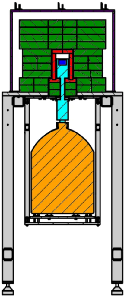
The MALBEK shield was designed by engineers at the Triangle Universities Nuclear Lab-oratory and is shown schematically in Figure 2.1. The detector and liquid nitrogen dewar can be lifted into the shield from below with a pallet jack. This eliminates the need to disas-semble the shield to access the detector, reducing the risk of shield component contamination from improper handling. The outermost shielding layer is 25.4 cm of polyethylene decking material that is not shown in Figure 2.1. Polyethylene has a high neutron capture cross section and is used to block (α,n) and fission neutrons from the cavern walls [34]. Inside the polyethylene is a sealed Lexan box that is continuously purged with dry boil-off nitrogen to reduce radon levels near the detector. The innermost shielding layers are made from lead. A 20 cm outer lead layer is built from 180 low-background lead bricks purchased from Sullivan metals with 210Pb activity less than 2.5 Bq/kg [35]. Each brick was etched in a nitric acid
inserted into the shield for detector calibrations.
Figure 2.1: Drawing of the MALBEK shield. The support table (grey) is approximately 140 cm tall. The germanium crystal (dark blue) sits within a copper vacuum cryostat (light blue). The innermost shield layer is made from ancient lead (red). This is surrounded by Sullivan lead (green) and a Lexan box that is flushed with boil-off nitrogen. The detector and dewar (goldenrod) can be lowered from the shield without unstacking the lead bricks. The polyethylene outer shield layer is not shown. Drawing is courtesy of Matthew Busch.
Section 2.2: Data Acquisition System and Slow Controls
language,ORCAScript, that can be used to automate data taking routines, monitor detector systems and data quality, and plot and filter the data stream in real-time. ORCA is used for all of the MALBEK data readout and slow control operation. An overview block diagram of the MALBEK data acquisition system is shown in Figure 2.2.
Figure 2.2: Block diagram of the MALBEK data acquisition system.
MALBEK is outfitted with a Canberra pulse-reset preamplifier with an approximately 40 ms reset period. The preamplifier has two identical signal outputs. One of the outputs is AC-coupled into a Struck Innovativ Systeme 3302 (SIS3302) eight-channel 16-bit 100-MHz VME digitizer. This channel has an energy range from 5 keV to 3 MeV and was used to study the MALBEK background spectrum around the 76Ge double-beta decay endpoint
SIS3302 signal channels self-trigger on the output of an on-board trapezoidal filter, which helps discriminate low amplitude signals from noise. The preamplifier pulse-reset signal, which indicates when a pulse-reset occurs, is also digitized by the SIS3302. When the reset channel is triggered a small data record containing the timestamp of the reset is placed in the
ORCAdata stream. In order to reduce the size of MALBEK data files, basic real-time filtering is implemented using ORCAScript to remove events associated with preamplifier resets that are easily distinguishable based on their shape. This filtering is not 100% efficient and offline pulse-reset event removal is also performed.
An Agilent 33220A arbitrary waveform generator is attached to the test input of the preamplifier and injects a test pulse at 10 sec intervals during data taking. The waveform generator events provide a useful means of tracking the detector resolution and stability over the long run periods. A sync pulser from the waveform generator is fed into a channel of the SIS3302 so that a record is captured in theORCAdata stream coincident with every waveform generator induced event. The waveform generator output can optionally be attenuated using a set of step attenuators controlled by an Acromag IP408 digital I/O VME module. This system is used to generate sets of events with a known waveform shape and energy. These events are then used to test the trigger efficiency of the digitizer and measure cut acceptance efficiencies near the detector energy threshold.
The detector is biased using an ISEG VHQ224L, a 5 kV VME-based high voltage supply with selectable polarity. The ISEG has peak to peak ripple less than 2 mV and can ramp the high voltage on or off at a programmable rate. The VHQ224L is controlled and monitored by ORCA.
accelerometer is attached to the detector stand and triggers on accelerations greater than 190 µg. This was intended to provide a record of vibrations caused by haul trucks passing the laboratory building or other mining operations that could cause microphonic events. No vibration events were recorded during the run period, perhaps due to the sheer mass of the shield and the isolation provided by the shipping container.
There are several systems in place to protect the detector in the event of a power outage or liquid nitrogen shortage. The entire data acquisition system is on an uninterruptible power supply capable of supporting the system for several minutes. Upon loss of power, the high voltage bias of the detector is ramped down by ORCA. If power is maintained but liquid nitrogen levels fall below a set point, the detector is automatically unbiased by the data acquisition computer. In the event of a computer failure that occurs simultaneously with a loss of liquid nitrogen, a custom circuit will automatically un-bias the detector.
AnORCAScriptis used to automate MALBEK data taking. New runs begin hourly. The
script collects run statistics, including channel trigger rates, energy spectra, and the status of slow control systems, like liquid nitrogen levels and bias supply current, and sends a daily summary email to users. The script also watches for excursions from standard operating conditions, such as liquid nitrogen fills or loss of power, and sends alert emails to a subset of the user group.
2.2.1: Digitizer Configuration
the spectral peak due to pulser events. The tau factor was determined by fitting the decay time of a set of physics waveforms collected with the SIS3302. The energy calculated by the digitizer trapezoidal filter was used for data quality monitoring. For physics data analysis, an offline energy reconstruction was performed. This is described in Section 2.4.1.
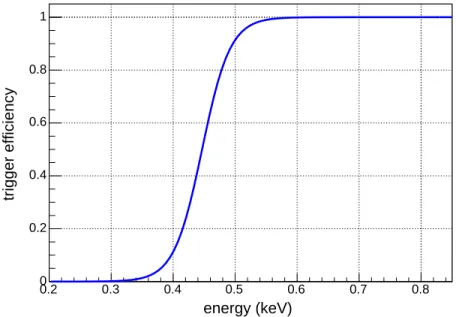
The SIS3302 also uses a fast trapezoidal filter for internal triggering to minimize the noise trigger rate near the detector threshold. When the filter output exceeds the channel’s trigger threshold, a prescribed number of analog-to-digital converter (ADC) values are stored in the event memory. The SIS3302 fast trapezoidal filter has three configurable settings: decimation, peaking time, and sum-gap time, which is the sum of the peaking time and the gap time. The same peaking and gap time found to optimize the energy filter were used for the trigger filter. The optimal trigger threshold maximizes the trigger efficiency for low energy events while maintaining a manageable noise trigger rate. A 300 eV trigger threshold was used during MALBEK data taking, about two times higher than the measured full width at half maximum (FWHM) of a pulser peak. Figure 2.3 shows the trigger efficiency as a function of energy determined using the waveform generator and attenuators.
energy (keV)
0.2 0.3 0.4 0.5 0.6 0.7 0.8
trigger efficiency
0 0.2 0.4 0.6 0.8 1
A user defined number of raw data samples are saved after every trigger. If the rising edge of an event is centered in the data buffer, the data sample length must only be twice the length of the energy trapezoidal filter to perform offline energy reconstruction. However, the position of the rising edge of the waveform changes with variations in the rise-time of an event, up to the length of the trigger trapezoidal filter peaking time. To accommodate this, an additional trigger filter peaking time of samples were added to the buffer length. Then the buffer length was rounded up to the nearest power of two, eliminating the need to truncate a waveform before performing frequency analyses, e.g. the wavelet denoising described in Section 3.3.1. 8192 samples were recorded for each event during data taking.
The location of an event’s rising edge within the buffer can be manipulated in two ways. The original SIS3302 firmware had a pre-trigger delay setting that defined the number of samples written to event memory before a trigger, up to a maximum length of 1024 samples. During initial testing with the SIS3302, it was found that the maximum pre-trigger delay was too short to digitize sufficient baseline to perform offline filtering on very slow events. A new firmware specification was provided to Struck engineers who implemented a feature called buffer wrap. The buffer wrap writes a constant stream of ADC data to the event memory, keeping a programmable number of samples in the buffer. After a trigger, the remainder of the event buffer is filled with post-trigger data. This allows for arbitrarily long pre-trigger delays at the expense of increased digitizer dead time as the event memory is refilled after each trigger. The buffer wrap delay was set during data collection to place the rising edge of the slowest rise-time events in the center of the digitization window.
The SIS3302 has a programmable offset that determines the position of the waveform within the 16 bit range of the digitizer. This was set so that the resting baseline of the preamplifier had an ADC value of approximately 5000. This allowed for a large ADC range for positive valued physics events while maintaining the ability to fully digitize triggers caused by signals that oscillate about the baseline, e.g. microphonics.
clear that there were bursts of noise present on the SIS3302 waveforms at 15 µs intervals. It was eventually determined that the noise originated from the VME-based single board computer (SBC) used to read out and control the SIS3302 and VHQ224L. To eliminate this noise, a readout scheme was implemented in ORCA that takes advantage of the dual data buffers on the SIS3302. During normal operation, the SIS3302 writes data to one of its buffers. The SBC does no polling at this time. At a set interval, the SBC polls the card and reads data from the first buffer. While this is happening, the SIS3302 writes any triggered event records to the second buffer. Once readout is complete, the SIS3302 begins writing to the original buffer and data written to the second buffer is discarded. This readout method eliminates the SBC polling related noise while reducing the detector lifetime by1%.
Section 2.3: MALBEK Operation History
MALBEK arrived at the University of North Carolina at Chapel Hill in October of 2009. After initial detector testing and basic characterization measurements, MALBEK was moved to its permanent location at KURF in January of 2010. The first year of MALBEK operations underground were spent testing data acquisition system configurations for use with theMajorana Demonstrator. Data collection using the SIS3302 digitizer described in Section 2.2 began in March 2011. After a modest dataset was collected with MALBEK in the shield, it became evident that a significant and unexpected peak at 46.5 keV originating from 210Pb was present in the data. This peak was accompanied by the set of lead x-rays between 70 and 90 keV and a bremsstrahlung continuum. Several possible sources of the
210Pb contamination were identified: brass components within the cryostat, tin solder used
MALBEK was removed from the shield on 24 October 2011 and the detector was driven from KURF to Canberra Industries in Meriden, Connecticut. At Canberra, the lead shims were removed and replaced with low-background PTFE. The data collected during this period are not suitable for a WIMP search due to the significant background contribution from
210Pb in the region of interest. However, the 210Pb contamination provided a useful low
energy gamma-ray calibration source inside of the cryostat that will be discussed in detail in Chapter 3.
The detector returned to KURF on 26 October 2011, after spending less than three days on the surface. The detector was inserted into the shield and cooled and data taking commenced on 15 November 2011, 12 days after the surface exposure. The detector continued to collect data for 288 days until 8 August 2012, at which point it was removed from the shield to perform a set of source calibrations that are discussed in Chapters 3 and 4. The data collected over the 288 day period are divided into two distinct run periods separated by a period of frequent power outages at KURF, 15 November 2011 – 12 March 2012, during which 104 days of data were collected, and 9 April 2012 – 29 August 2012, during which 117 days of data were collected. The data processing and calibration described in Section 2.4 is performed separately on these two run periods.
Section 2.4: Data Processing
Before data collected withORCAcan be used to search for a signal, the data are processed and basic data selection cuts are applied. A comprehensive overview of the MALBEK data processing and selection can be found in [33]. A general overview will be given here.
collaboration for analyzing HPGe detector data [39]. GAT is a collection of processors that calculate parameters from an event, e.g. the event energy and rise-time. After the data are processed with GAT, the event energies are calibrated and cuts are applied to remove noise and other non-physics related signals.
2.4.1: Energy Calculation and Calibration
Event energies are calculated using a digital trapezoidal filter [37] implemented as a processor in GAT. First, event waveforms are pole-zero corrected to remove the decaying component of the signal caused by AC-coupling the pulse-reset preamplifier into the SIS3302 digitizer. The waveform is then filtered using a trapezoidal filter with an 11.0 µs peaking time and a 1.0 µs gap time. The maximum value of the filtered waveform is used as the uncalibrated energy of the event. The optimal peaking time and gap time were found by minimizing the resolution of a pulser energy peak by varying the two parameters.
MALBEK’s copper cryostat and thick n+ contact severely attenuate low energy gamma-rays and x-gamma-rays from external radioactive sources, so the energy calibration utilizes several x-ray peaks from cosmogenically activated isotopes within the germanium crystal. The peaks listed in Table 2.1 are fit with a gaussian function and a linear background function. The peak centroids are then fit with a linear equation to determine the conversion between the trapezoidal filter energy and ionization energy. This calibration is done separately for the two data taking periods.
Table 2.1: Peaks used for energy calibration. Peak energies are from [40].
Isotope Energy (keV)
2.4.2: Data Selection Cuts
After processing the data with GAT, a series of cuts are applied to remove non-physics events. Two general classes of cuts are performed, cuts based on the timing of the event and cuts based on the waveform shape. For a detailed description of the definition and performance of these cuts, see [33].
The first timing based cut removes data runs collected immediately following detector re-biasing after a power outage. These runs were found to have increased trigger rates and can be eliminated without a significant impact on the down-time of the detector relative to the exposure lost during the power failure. The second timing based cut removes events that occur within 1 ms of a pulse-reset signal from the preamplifier. The preamplifier resets at approximately 25 Hz, so this cut reduces the live-time of the detector by about 5%. In a similar fashion, events that are coincident with the waveform generator signal are cut from the dataset. Lastly, the 15 minutes of data collected following a nitrogen fill are removed. The trigger rate over this time period temporarily spikes, likely due to microphonics caused by boiling nitrogen in the dewar and fill lines.
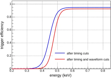
oscillatory noise events identified by the integral cut as well as the inverse polarity micro-discharge events. The final waveform shape based cut uses the ratio of energies calculated by two trapezoidal filters with different shaping times [41]. This cut identifies any remaining microphonic events that are not removed by the integral and A/E cuts. The calculated signal acceptance efficiency after application of the timing and waveform shape cuts is shown in Figure 2.4.
energy (keV)
0.2 0.3 0.4 0.5 0.6 0.7 0.8
trigger efficiency
0 0.2 0.4 0.6 0.8 1
after timing cuts
after timing and waveform cuts
Figure 2.4: Basic data selection cut efficiencies. The signal acceptance efficiency after ap-plication of the timing cuts is shown in red and the signal acceptance efficiency after the timing cuts and waveform shape based cuts are applied is shown in blue.
CHAPTER 3: Surface Events
Section 3.1: Signal Formation in PPC Detectors
Ionizing radiation incident on a High Purity Germanium (HPGe) detector will create electron-hole pairs proportional in number to the total energy deposited in the detector. Any mobile electrons (holes) created within the crystal’s depleted region will drift towards the n+(p+) detector contact under the influence of the electric field generated by the applied
bias voltage and the space charge distribution within the detector. As the charges move, they induce currents on the contacts that are dependent on the number and velocity of the charge carriers and the field they are moving through. A single charge carrier q will induce a charge Q on an electrode
Q=−qφ0(x) (3.1)
whereφ0(x) is the weighting potential that describes the coupling of a charge carrier within
the detector to a given electrode [42]. The weighting potential is calculated by setting the electrode of interest at a unit potential and all other electrodes at zero potential. Equation 3.1 provides a means of determining the signal that results from a particle interacting within a detector and creating electron-hole pairs. First, the mobile charges’ paths through the crystal are calculated. These depend on the charge drift velocity as a function of field and crystal orientation and the motion of charge carriers due to diffusion and mutual repulsion. Then, the calculated charge trajectories are combined with the weighting potential to determine the induced current on the corresponding electrode.
the preamplifier will be proportional to the total number of electron-hole pairs created by the original interaction. While the amplitude of the signal will be the same for a given amount of energy deposited, the time evolution of the voltage signal is influenced by the topology of the charge carriers, the geometry of the detector, and the characteristics of the electric field within the crystal. Traditional detector geometries, like the coaxial and planar configurations often used for gamma ray spectroscopy, have smoothly varying weighting fields, short drift paths, and short collection times. This results in signals with consistent shapes regardless of the interaction position of the incident particle.
Figure 3.1: Weighting potential within a PPC detector. The color intensity shows the magnitude of the weighting potential throughout the bulk of the detector. The white lines show calculated hole drift paths. The weighting potential and drift paths were calculated using M3DCR [43] and SigGen [44]. Figure is from [33].
means that holes created at different locations within the crystal may arrive at the point contact at varying times. These two features, a sharply peaked weighting potential and position dependent drift times, result in signal shapes that vary markedly with event type.
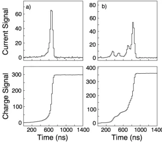
Figure 3.2 shows an example of the varying signal shapes seen using a PPC detector. A gamma-ray that Compton scatters within the detector can deposit energy in two or more locations. The charge created at each interaction point may reach the high weighting po-tential region of the detector at different times, inducing current signals on the electrode that can be resolved in time, as seen in panel (b). A gamma-ray that is photoelectrically absorbed within the detector, depositing all of its energy in a single location, will induce a single discrete current signal, as seen in panel (a). The dependence of signal shape on inter-action position in PPC detectors can be used to distinguish multi-site events from single-site events, a valuable background rejection technique when searching for a single-site event like neutrinoless double-beta decay in the presence of gamma-ray backgrounds.
Section 3.2: Surface Events in PPC Detectors
The n+ contact of a PPC detector is created by depositing lithium on the surface of the detector and diffusing it into the crystal lattice, resulting in an approximately 0.5 - 1 mm thick region of n+material extending from the surface into the bulk of the detector. Because
of the high impurity concentration in this region, much of the n+ contact volume remains
un-depleted when the detector is biased. For many PPC detector applications, e.g. gamma-ray spectroscopy, where relevant energies often don’t fall below 30 keV, this layer is assumed to be entirely inactive when determining the absolute efficiency of the detector to a given photo-peak. In low-background applications, the inactive layer has the desirable property of preventing alpha radiation from the 232Th and the 238U decay chains from entering the detector bulk [45].
In reality, the surface region of the crystal is not entirely inactive. Some fraction of the charge created by an interaction within the n+ layer can diffuse into the depleted region of
the detector and induce a signal in the same manner as a bulk interaction. The amplitude of the signal will only reflect the fraction of initial charge carriers that move into the depletion region, and the full energy of the originating interaction will be lost. Because of this, surface layer events can populate all energies below the full energy of the original interaction.
Spectra showing 40 days of data collected with MALBEK, both before and after the removal of the lead shims described in Section 2.3, are shown in Figure 3.3. The basic data selection cuts described in Section 2.4.2 have been applied to both spectra. The data collected with the lead shims in the cryostat shows a significant peak at 46.5 keV from210Pb and a roughly exponentially increasing population of events at low energies. The events in this continuum are hypothesized to be energy degraded signals caused by 210Pb
gamma-rays, x-gamma-rays, and bremsstrahlung interacting in the surface region of the detector. The 40 day spectrum collected after removal of the lead shims shows a factor of 10 decrease in both the 46 keV peak and the continuum of surface events.
partic-energy (keV)
5 10 15 20 25 30 35 40 45 50
-1
d
-1
kg
-1
counts keV
0 20 40 60 80 100
Figure 3.3: Comparison of energy spectra before (blue) and after (red) the removal of lead shims containing relatively high levels of 210Pb from the cryostat. The 46.5 keV 210Pb
gamma-ray peak is clearly present in the pre-shim removal energy spectrum along with an increased number of events at low energies caused by interactions occurring near the surface of the detector. The post-shim data shows a factor of 10 reduction in the 46.5 keV line and correspondingly fewer events at low energies.
present on the waveform. The remainder of this chapter will discuss various techniques for identifying surface events and evaluating the acceptance and rejection efficiencies of surface event removal cuts.
energy (keV)
1 2 3 4 5 6
-1
d
-1
kg
-1
counts keV
0 50 100 150 200 250 300 350 400
Figure 3.4: Expected signal from 15 GeV WIMPs recoiling from Ge nuclei (red dashed) and a spectrum from 40 days of data taken with the MALBEK detector with lead shims in the cryostat. The spectrum and expected WIMP signal exhibit similar shapes. The MALBEK events in this region are primarily due to the large surface event background from 210Pb
gamma-rays and x-rays interacting near the n+ contact.
Section 3.3: Surface Event Identification
electrode, resulting in charge signals that take several microseconds to reach their maximum value. This is in sharp contrast to events that occur in the bulk, where all holes are collected through the high field region in several hundred nanoseconds. The difference in the event rise-time, the time it takes the charge signal to reach its maximum value, can be used to distinguish bulk events from surface events and, ultimately, remove surface events from the dataset.
s) µ time (
0 1 2 3 4 5 6 7 8 9 10
fraction of charge collected
0 0.1 0.2 0.3 0.4 0.5 0.6 0.7 0.8 0.9
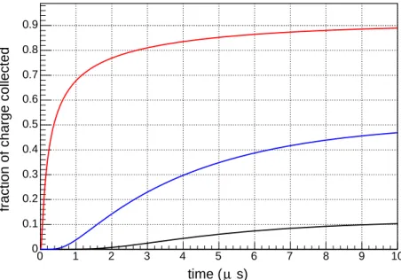
Figure 3.5: Fraction of the charge reaching the surface-bulk boundary as a function of time for a 2D model of a 1 mm deep surface layer. Charges are initially deposited at depths of 0.1 mm (black), 0.5 mm (blue), and 0.9 mm (red). It takes several microseconds for charge to diffuse into the bulk, resulting in charge signals with long rise-times. For a more complete discussion of slow event formation and modeling, see Chapter 4.
time (ns)
37000 38000 39000 40000 41000 42000 43000 44000 45000 46000
voltage (au)
0 20 40 60 80 100
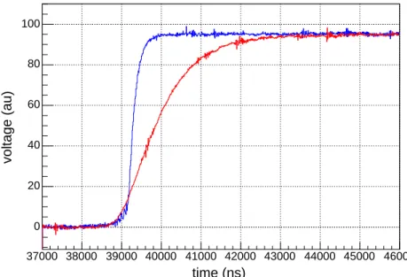
Figure 3.6: Waveforms from a 40 keV bulk event (blue) and a likely 40 keV surface event (red). The surface event takes over 3µs to reach its maximum value. The bulk event reaches its maximum value in approximately 500 ns.
3.3.1: t10−90 Rise-time
A straightforward method for determining the rise-time of an event is to calculate the time it takes the charge signal to rise from 10% to 90% of its maximum amplitude, t10−90[31, 46].
This is done by determining the maximum and minimum amplitude of the charge pulse, then scanning along the waveform to find the points at which the waveform rises by 10% and 90% of the maximum. This method performs well when the signal-to-noise ratio is high, but can be inaccurate as the signal amplitude decreases. An example of this is shown in Figure 3.7, which shows the difference in the rise-time calculated for a set of waveforms when the 10% and 90% points are found by scanning away from the mid-point of the waveform and when the 10% and 90% points are found by a scan starting at the beginning and the end of the waveform.
The failure to correctly determine t10−90, as demonstrated in Figure 3.7, is often a
energy (keV)
0.5 1 1.5 2 2.5 3 3.5 4
s)
µ
difference (
10-90
t
0 5 10 15 20
Figure 3.7: The difference in the calculated rise-time using two methods as described in the text for finding the 10% and 90% of maximum points as a function of energy. Above 2 keV, there is no difference in the calculated rise-time between the techniques. As the signal-to-noise ratio decreases below 2 keV, the two rise-time calculation techniques give different results. Between the 0.6 keV threshold and 0.8 keV, almost 50% of the waveforms have inconsistent t10−90 calculations.
failed because of a noisy feature occurring at 38,500 ns. In this case, it is necessary to perform some sort of digital filtering to remove the noise from the waveform while leaving the frequencies relevant for the rise-time calculation intact. A commonly used method for removing noise from a signal without broadening its features is wavelet denoising, also known as wavelet thresholding [47–50].
trans-time (ns)
36000 37000 38000 39000 40000 41000 42000
voltage (au)
-20 0 20 40 60 80
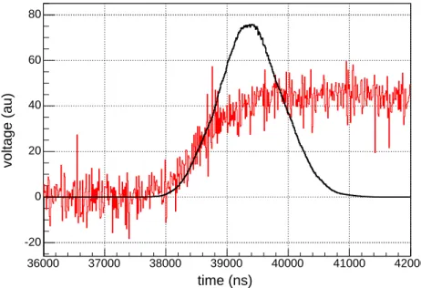
Figure 3.8: A 3.2 keV waveform (red) and the same waveform after wavelet de-noising (black). Arrows indicate the t10 and t90 times calculated using the raw waveform (red) and
the de-noised waveform (black). The t90 calculated using the raw waveform is incorrect due
to noise on the rising edge of the signal.
form (DSWT) is used for the forward and inverse waveform transformation. The DSWT is translation invariant and eliminates artifacts caused by alignment between the signal and the basis wavelet, a common problem in schemes that utilize the discrete wavelet transform (DWT) [53]. Eight levels of the DSWT are performed on MALBEK waveforms. The choice of the optimum level for denoising depends on the signal and noise characteristics of the data and is best found through experimentation. A favorable waveform basis is selected by maximizing the cross-correlation between the wavelet and the signal. In this analysis, a Haar wavelet is used as a mother wavelet due its close resemblance to a PPC signal. Hard thresholding is performed on each level of decomposed waveform following [48] and defining the threshold values using a set of pure noise events collected by randomly triggering the data acquisition systems. The literature on wavelet theory and wavelet denoising is vast. Some useful texts on the subject are [54–56].
black arrows, doesn’t suffer the same noise sensitivity as the t10−90 calculation performed on
the original waveform and more accurately reflects the true rise-time of the event. While wavelet denoising improves the performance of the t10−90 calculation, it is not a panacea.
Figure 3.9 shows the t10−90 calculation performed on a set of events generated using the
waveform generator and attenuator system described in Section 2.2. Events in this dataset have a t10−90time of about 450 ns and span energies from 300 eV to 6.7 keV, providing a useful
means of testing the efficacy of rise-time determination techniques around the 600 eV detector threshold. As the signal-to-noise decreases, so does the accuracy of the t10−90 calculation
of the denoised waveforms. Below 3 keV, the rise-time calculation behaves unpredictably, rendering the t10−90 time ineffective as a means to distinguish surface from bulk events.
With this result in mind, efforts were made to define a parameter correlated with the event rise-time but less sensitive to noise.
energy (keV)
1 2 3 4 5 6 7
s)
µ
(
10-90
t
0 0.5 1 1.5 2 2.5 3 3.5 4
0 20 40 60 80 100 120
Figure 3.9: t10−90 versus energy for a dataset generated using an arbitrary waveform
genera-tor. The test signal is stepped down in amplitude in discrete intervals from 6.7 keV to below the detector threshold. All of the events have t10−90 rise-times of 450 ns, but as the
3.3.2: wpar
Mallat’s algorithm decomposes the wavelet transformation into a cascading series of fil-ters [57]. At each level of the transformation, the signal passes through a set of high pass and low pass filters determined by the properties of the mother wavelet. The output of the low pass (integrating) filters are called approximation coefficients and reflect the gross properties of the waveform at the scale (frequency band) of the level. The output of the high pass (differentiating) filter are called detail coefficients and are sensitive to the higher fre-quency components at that scale. When performing a DWT, the approximation coefficients are down-sampled before being passed to the next level of filtering, while the DSWT passes the un-decimated approximation coefficients. This is a redundant scheme, but overcomes the translation variance of the DWT that can cause artifacts in the denoised waveform. A graphical representation of the DSWT is shown in Figure 3.10.
Figure 3.10: Block diagram representing a three level discrete stationary wavelet transforma-tion (DSWT) of waveform X[i]. H0 is a high pass filter block resulting in detail coefficients
dn[i], where n is the level of the filter, and G0 is a low pass filter block resulting in
approxi-mation coefficients cn[i]. The un-decimated approximation coefficients from level n pass to
the level n+ 1 filters.
In [33], a parameter is developed that is sensitive to the rise-time of a waveform based on the detail coefficients calculated during the DSWT. The formal definition is
where c(Di)(n = 0) is the ith first-level detail coefficient and E is energy of the event. The behavior of wpar is dependent on the specific choice of wavelet, the number of transform
levels used, and the waveform sampling frequency. For MALBEK, the DSWT is an 8-level transformation using a Haar wavelet, so the level-1 coefficients are the average of 28 adjacent
samples, or 2.6 µs of waveform, minus the average of the next 28 samples. c(i)
D(n = 0) is
effectively a smoothed derivative of the waveform. Taking the absolute value squared of c(Di)(n = 0) follows the convention for obtaining power spectra in frequency analysis and dividing byE2 normalizes the squared derivative by its amplitude. The result is thatwpar is
simply a measure of the maximum slope of the waveform, smoothed, squared, and normal-ized. An example calculation of wpar is shown in Figure 3.11.
time (ns)
36000 37000 38000 39000 40000 41000 42000
voltage (au)
-20 0 20 40 60 80
Figure 3.11: A 3.2 keV waveform (red), identical to the waveform show in Figure 3.8, and the first level detail coefficient power spectrum (black). The maximum value of the power spectrum normalized by the energy of the event squared (wpar) is used as an alternative
calculation of the event rise-time.
Figure 3.12 shows the wpar distribution for the same set of waveform generator events
shown in Figure 3.9. The spread in the distribution of the calculated wpar value increases as
the signal-to-noise decreases, but, in contrast to t10−90, it does so in a smooth,
energy (keV)
1 2 3 4 5 6 7
par
w
10 20 30 40 50 60
0 10 20 30 40 50 60
Figure 3.12: wpar versus energy for a dataset generated using an arbitrary waveform
gener-ator. All of the events have t10−90 rise-times of 450 ns. The spread in calculatedwpar values
increases with decreasing energy, but does so in a way that is more easily characterized than the t10−90 distribution shown in Figure 3.9.
energy (keV)
1 2 3 4 5 6 7
par
w
10 20 30 40 50 60
0 10 20 30 40 50 60 70
Figure 3.13: wpar versus energy for a dataset generated using an arbitrary waveform
Figure 3.13 shows the wpar distribution for a set of waveform generator events with t10−90
rise-times of 1100 ns. The shape of the distribution is similar to Figure 3.12, but the mean wparvalue is lower. The remainder of the analyses described here will utilizewpar to evaluate
the rise-time of events. It is important to note thatwparis not the inverse rise-time, although
they are clearly related in a manner that is dependent on the detailed shapes of the wave-forms produced by the detector. However, they need not be related in the first place. The only requirement for this analysis parameter is that it separates bulk from surface events. Figure 3.14 shows the t10−90 value and the wpar value calculated for events collected using
the MALBEK detector with lead shims in the cryostat. Above 2.5 keV, wpar is clearly
sen-sitive to the rise-time of the event. Below 2.5 keV, the poor performance of t10−90 makes a
comparison to wpar uninformative. Section 3.4 will describe the performance of wpar in the
lowest energy regime and discuss how wpar can be used to remove surface events with slow
rise-times from a dataset.
par
w
10 15 20 25 30 35
s)
µ
(
10-90
t
0 0.5 1 1.5 2 2.5 3
0.6 - 2.5 keV
2.5 - 6.0 keV
6.0 - 10.0 keV
Figure 3.14: t10−90 versus wpar for events in three different energy regions. These data were
collected with lead shims in the detector cryostat. Between 6.0 and 10.0 keV (violet) there is a clear correlation between event rise-time and wpar. The same is true between 2.5 and
Section 3.4: Surface Event Removal
Before performing a search for a signal from new physics with a PPC detector, slow surface events, which can constitute a significant background, must be quantified or removed from the data. When there is overlap between signal events and background events, e.g. the region of the spectrum below 2 keV, there are two paths one could take to accomplish this. The first is to define a cut that maximizes the acceptance of bulk fast events, and hence the exposure of the detector, and then correct for any slow surface events that pass the cut criteria and contaminate the signal region of interest. The second option is to define a cut that more efficiently removes surface events, but necessarily does so at the expense of the fast event acceptance efficiency. In both approaches, failure to properly correct for the slow event contamination or the acceptance efficiency of fast events can artificially improve or reduce the sensitivity of the experiment, or, at worst, mimic the very signal one is looking for.
This section will examine the distribution of slow surface events and the effect of various cuts on populations of slow and fast events in different datasets, ultimately showing that a measurement of the signal acceptance efficiency is more accurate and reliable than a mea-surement of the background leakage. Bulk signals have a more-or-less universal shape that can be mimicked with a waveform generator or using attenuated data, and the evaluated signal efficiency can be cross-checked using known spectral features, such as the stability of the L-shell line strength as a function of the cut. Measuring background leakage, on the other hand, requires a good model of or proxy for the various populations of background sources in this energy range, which are difficult to obtain.
3.4.1: Surface Event Distributions From Varying Sources
presented in this section. The first is 40 days of data collected with a210Pb source inside of
the cryostat, the second dataset is a thirty minute run taken with an uncollimated 241Am
calibration source positioned directly above the cryostat on-axis with the detector, and the last dataset consists of 89.5 kg-d of shielded exposure used for the analyses presented in Chapter 5.
Figure 3.15a shows the wpar distribution for events in the 0.6 keV to 50 keV energy range
for the 40 day lead source dataset. Figure 3.15b shows data over the same energy range collected during an equivalent exposure time after the lead shims were removed. Energy spectra from these datasets were previously shown in Figure 3.3. The number of events in the 46 keV 210Pb peak are reduced by an order of magnitude in Figure 3.15b. The same
reduction is seen in the band of slow events with wpar values less than 30, demonstrating
that radiation, in this case external 46 keV gamma rays, lead x-rays ranging from 70 to 90 keV, and lead bremsstrahlung interacting near the detector surface populate the slow event continuum down to the detector energy threshold. Events that are postulated to occur near the detector surface have both longer rise-times and lower signal amplitudes, consistent with the simple model of charge diffusion shown in Figure 3.5. Below 2 keV, the slow event band bleeds into the fast event region. This contamination must be accommodated when performing a slow event cut based on wpar.
The wpar distribution for data collected with an uncollimated 241Am source illuminating
(a)
(b)
Figure 3.15: wpar distributions for 40 days of data taken before (a) and after (b) removal of
the 210Pb contamination in the cryostat. In (a), the continuum of slow events is due 46 keV
ray source’s position relative to the crystal. The band of slow events with wpar values less
than 30 are clearly separated from the fast event population at 10 keV but bleed into the fast pulse region at energies less than 2 kev. This is further illustrated by the two curves in Figure 3.16. The solid red line is defined such that 99% of fast rising events generated with the pulser fall above the line. The solid green line is defined so that 99% of the events in the 241Am dataset fall below the line. Assuming the majority of events in the241Am dataset below 12 keV are energy degraded surface events, the solid green line is an approximation of where one would place a cut to efficiently remove slow events. There is a significant region below 2.5 keV where events fall below the slow event rejection curve and above the fast pulse acceptance curve. Events in this region are ambiguously defined. Again, any cut that is designed to retain fast events from this region must correct for slow event leakage into the signal region.
Figure 3.16: wpar versus energy for a flood measurement using an 241Am source. All events
falling above the solid red curve pass a rise-time cut built to retain 99% of fast pulser data. Events falling below the solid green curve fail a cut designed to remove 99% of the 241Am
data. Between the two curves is an ambiguous region containing events identified as both surface and bulk events.
K-shell capture (9.0 keV),68Ga K-shell capture (9.7 keV), and68Ge K-shell capture (10.4 keV)
lines are visible as tight clusters aroundwpar values of 30. The corresponding L-shell capture
lines are visible around 1 keV, forming a vertical band. This band demonstrates the same spread inwparvalue that is visible in the fast pulser data as the signal-to-noise ratio decreases
towards the detector energy threshold. The 89.5 kg-d dataset has a smaller contribution from slow events than the lead shim or241Am datasets. Still, the contamination of the fast event region from the slow event continuum below 2 keV is visible in the figure.
Figure 3.17: wpar versus energy for the 89.5 kg-d exposure dataset.
To better understand the differences in slow event populations from different background sources, it is instructive to examine wpar distributions within a fixed energy window.
Fig-ure 3.18a shows the distribution ofwpar values for events falling between 0.6 keV and 0.9 keV
for the 241Am source data, lead shim data, 89.5 kg-d exposure, and the fast waveform
gen-erator dataset. In this energy region, spanning from the detector threshold to 3σ below the
65Zn L x-ray line, the three physics datasets consist mostly of slow events. The slow event