Modelling Digital Quantum
Simulation of the Rabi Model in
Circuit QED:
Towards an Experimental Implementation of
Deep-Strong Coupling Dynamics
THESIS
submitted in partial fulfillment of the requirements for the degree of
MASTER OF SCIENCE in
PHYSICS
Author : Marios Kounalakis
Student ID : 1455745
Supervisor : Leonardo DiCarlo
Modelling Digital Quantum
Simulation of the Rabi Model in
Circuit QED:
Towards an Experimental Implementation of
Deep-Strong Coupling Dynamics
Marios Kounalakis
Huygens-Kamerlingh Onnes Laboratory, Leiden University P.O. Box 9500, 2300 RA Leiden, The Netherlands
PROJECT UNDERTAKEN AT
Quantum Transport Group Kavli Institute of Nanoscience Delft University of Technology
Lorentzweg 1, 2628 CJ Delft, The Netherlands
SUPERVISED BY
iv
Abstract
The simplest form of dipole interaction between an atom and a single photon field mode, is described by the vacuum Rabi model. Strong atom-photon coupling, which is described by the simpler Jaynes-Cummings model, has been achieved in many platforms, such as cavity and circuit quantum electrodynamics (QED) and has brought a lot of success towards experimental quantum informa-tion processing over the past years. The full Rabi model dynamics can only be obtained in the so-called ultra-strong and deep-strong coupling regimes where the interaction coupling strength is com-parable or higher than the natural system frequencies. However, due to our inability to achieve such high coupling strengths, these regimes remain largely unexplored in the lab. In this thesis, we investigate the possibility of reaching these regimes in a circuit QED setup, by means of a recently proposed analog-digital quan-tum simulation. Following a detailed numerical model of the pro-posed scheme, where we include the most important experimental limitations, we demonstrate the feasibility of the proposal using a transmon coupled to a 2D superconducting resonator, for a certain range of design parameters. Moreover, we show that the Wigner function representation of the resonator state in phase space is in-strumental in order to probe the signature of deep-strong coupling in the system. Following these results, we design a device that will enable us to carry out the experiment with high fidelity measure-ments and perform direct Wigner tomography inside the resonator.
iv
Contents
1 Introduction 1
1.1 Quantum light-matter interactions 1
1.2 Simulating nature with quantum mechanics 2
1.3 Research focus and thesis overview 2
2 Theory 5
2.1 The vacuum Rabi model 5
2.2 Superconducting qubits 7
2.2.1 From the Cooper-pair box to the transmon 7
2.2.2 Circuit quantum electrodynamics 9
2.3 Quantum simulations 10
2.3.1 Analog and digital implementations 10 2.3.2 An analog-digital quantum simulation of the Rabi
model in circuit QED 11
3 Numerical model description 15
3.1 The need for a numerical simulation 15
3.2 Master equation 16
3.2.1 Master equation for the transmon-resonator system 16
3.3 Rotating frame transformation 17
3.4 Implementing the drive 18
3.4.1 DRAG pulses 20
3.5 Flux control of qubit frequencies 21
3.6 Trotter step description 24
4 Numerical results 27
4.1 Simulations for ideal two-level qubits 27
vi CONTENTS
4.1.2 Finite time Trotter steps: Slowing down the dynamics 28 4.1.3 Eliminating first order Trotter errors 29 4.1.4 Simulations for various coupling strengths 32 4.2 Simulations for a realistic circuit QED setup 33 4.2.1 From qubit to transmon - adding the third level 33
4.2.2 Dissipation 34
4.2.3 Finite-bandwidth flux control: RC filter 37 4.2.4 Final real-world quantum simulations 38 4.3 Exploring the dynamics of the deep-strong coupling regime 39
4.3.1 Strong coupling and beyond 39
4.3.2 Superpositions of coherent states 40 4.3.3 Hybrid discrete - continuous variable entanglement 43 4.3.4 Creating Schr ¨odinger cat states 46
5 Towards an experimental implementation: designing the chip 49 5.1 Overview of the experiment and readout process 49 5.1.1 Readout of qubit and cavity states 49
5.1.2 Wigner tomography 51
5.1.3 Schematic of the device 53
5.2 Main considerations in designing the parameters 54
5.2.1 Eliminating the Purcell effect 54
5.2.2 Suppressing non-linear terms 55
5.2.3 High fidelity qubit measurements 55
5.2.4 Summary of the designed parameters 56
5.3 Designing the chip elements 59
5.3.1 Resonator quality factors 59
5.3.2 Josephson junctions 61
5.3.3 Charging energy 61
5.3.4 Coupling strength 63
6 Conclusions and future work 65
vi
Chapter
1
Introduction
1.1
Quantum light-matter interactions
The simplest model for quantum light-matter interaction was introduced by Rabi in 1936 [1], and describes the dipolar coupling of a two-level atom with a single mode photon field.
The ability to experimentally achieve couplings that are much bigger than the system decay rates has allowed for an extensive study of this interaction in many platforms, including atoms and ions in strongly con-fined cavity field [2, 3], as well as microfabricated artificial atoms coupled to 2D and 3D gigahertz resonators [4]. Typically, coupling strengths are much lower than the natural frequencies in the system and the dynamics reduce to those of the Jaynes-Cummings model [5], following a rotating wave approximation (RWA) where only the excitations-conserving terms are considered. The exact solvability of this toy model and the developed dressed atom formalism involving coherent population Rabi oscillations, have enabled precise control of these systems which has led to many mill-stones in quantum state engineering [6].
2 Introduction
1.2
Simulating nature with quantum mechanics
Modelling and performing simulations of physical systems is a fundamen-tal part of the huge scientific and technological progress nowadays. With the power of today’s classical computers, researchers in almost all scien-tific areas are able to extract information about systems of interest with speed and precision beyond human capabilities. However, the complex-ity of quantum systems, makes it difficult to calculate their properties due to the Hilbert space dimensions growing exponentially with the number of particles, setting a limit in the number of systems that we can simulate exactly.
In 1982, R. Feynman proposed the idea of using a quantum simulator, instead of a classical one, to simulate such systems [10]. His vision was that, if we have a quantum system which we are able to control with high precision, then by tuning some of the parameters of that system we might be able to reveal information about another quantum system of interest that shares the same dynamics. Provided that we are able to engineer and control such a quantum device, the amount of time required for a calcula-tion will scale polynomially (not exponentially) with the number of parti-cles. Moreover, as S. Lloyd has demonstrated in 1996, a universal quantum simulator can be built by using digital methods [11]. In particular, he ob-served that the dynamics of any quantum system can be approximated by a sequence of operations in very small time steps, using the Trotter decom-position [12]. Therefore, the reproduction of the dynamics of any system should be possible by applying a series of well-controlled quantum gates at very short time steps.
Quantum simulations offer not only the possibility to perform exact calculations of complex quantum systems, but also to experimentally ac-cess phenomena that have never been observed or even not exist in na-ture. It is a highly expanding field with many potential applications in a number of areas in physics, chemistry or even biology [13]. In fact, many proof-of-principle experiments have been realised so far in a variety of platforms, such as cold atoms [14, 15], trapped ions [16, 17], NMR [18, 19] and superconducting circuits [20–22].
1.3
Research focus and thesis overview
In this thesis, we investigate the possibility of experimentally reaching the largely unexplored deep-strong coupling regime of the Rabi model in a circuit QED setup, by means of an analog-digital quantum simulation that
2
1.3 Research focus and thesis overview 3
has recently been proposed by A. Mezzacapoet al.[23]. We want to achieve this in a circuit QED setup, using a superconducting transmon qubit cou-pled to a transmission line resonator. Our goal is to investigate whether this proposal is feasible with current state of the art architecture, and if so, in what parameter regimes. For this reason, we build up a numeri-cal model description of the quantum simulations scheme including real-world experimental considerations of our system. Moreover, we want to understand the key features of the DSC dynamics and find possible ways to identify them in the experiment.
In chapter 2, we introduce the theoretical background as well as the motivations for this project. A brief description of the quantum Rabi model is followed by an introduction to circuit QED using superconducting trans-mon qubits. Finally, we present the ideas of universal quantum simula-tions and conclude with a description of the proposed analog-digital quan-tum simulation of the Rabi model in circuit QED.
In chapter 3, we present a step by step description of our numerical model. We discuss the master equation description of open quantum sys-tems and implement all the necessary elements for an accurate modelling of the proposed quantum simulations scheme.
In chapter 4, we present our numerical results concerning the feasibil-ity of the proposal in realistic circuit QED scenarios. Moreover, a detailed study of deep-strong coupling Rabi model dynamics is carried out in order to identify the key signatures of this regime.
In chapter 5, we describe the design of a chip based on these results. We implement all the necessary elements and design the key parameters for a high fidelity quantum simulation experiment.
Chapter
2
Theory
2.1
The vacuum Rabi model
The quantum Rabi model [1, 2] describes the simplest interaction between quantum light and matter, i.e. the dipolar interaction of a two-level atom (qubit) coupled to a single quantized electromagnetic field mode. The dy-namics of the coupled system are described by:
HR =h¯
"
ωRr a†a+
ωRq
2 σ
z+gR(
σ++σ−)(a†+a)
#
, (2.1)
where the last term describes the interaction between the atomic dipole (σ+ + σ−) and the photon electric field(a†+a), governed by the coupling strength gR. Here, a† and aare the creation and annihilation operators of the bosonic field and σ+ = |eihg|, σ− = |gihe|, σz = |gihg| − |eihe| are the Pauli operators of the qubit, where|giand |eidenote the ground and excited states, respectively. When the atom and photon frequencies are nearly on resonance (|ωRq −ωrR| gR), the interaction term is dominat-ing and the atomic and bosonic fields become strongly correlated with the exchange of photon excitations.
On the theoretical side, despite its simplicity, an exact analytical solu-tion of the quantum Rabi model in all parameter regimes has only been achieved recently by D. Braak [24]. More surprisingly, the generalised Dicke model [25] where N atoms are coupled to a photon field remains unsolvable forN >3.
6 Theory
Figure 2.1: Schematic of a two-level atom coupled to a quantised oscillator
mode.Figure obtained from [27]
frequencies (gR ωqR,ωrR) and following a rotating wave
approxima-tion (RWA) where the fast oscillating counter-rotating terms σ+a†, σ−a are neglected [26], the dynamics are accurately described by the Jaynes-Cummings model [5]:
H=h¯ωra†a+h¯
ωq
2 σ
z+g(
σ+a+σ−a†), (2.2)
which is exactly solvable.
Jaynes-Cummings physics have been studied extensively in many plat-forms, including cavity and circuit quantum electrodynamics (QED) [2, 4], where atoms/qubits are strongly confined in cavities/resonators. An ex-citation in these systems is coherently reabsorbed and re-emitted several times, leading to entanglement between the qubit and the resonator, for very long timescales. The ability to control these dynamics provides one of the most important physical resources towards quantum information processing.
As one increases the atomic and photonic frequencies with respect to the coupling strength, however, the RWA breaks down and the Jaynes-Cummings model is not sufficient to describe the dynamics. One enters the so-calledultra-strong(g/ωq,r &0.1) anddeep-strong(g&ωq,r) coupling
regimes of the Rabi model, that require the full Rabi Hamiltonian to be described.
6
2.2 Superconducting qubits 7
Although ultra-strong coupling has been confirmed in many setups including circuit QED [8, 9], the deep-strong coupling regime which con-tains counter-intuitive dynamics, still remains largely unexplored experi-mentally.
2.2
Superconducting qubits
Superconducting qubits are effective nonlinear oscillators behaving as ar-tificial atoms that are constructed by simple superconducting circuits based on LC oscillators [28]. A Josephson tunnel junction then introduces non-linearity to the system, such that one obtains anharmonic ocsillator be-haviour that renders it an artificial two-level atom.
Figure 2.2:Schematic of the anharmonic potential of a superconducting qubit.
The main advantage over other architectures is that the Hamiltonian parameters are effectively designed using advanced fabrication techniques. One can in principle distinguish three types of superconducting qubits, namely the charge (also known as ”Cooper-pair box”), the flux and the phase qubit.
2.2.1
From the Cooper-pair box to the transmon
The Cooper-pair box (CPB) [29] is a type of charge qubit, that consists of a small superconducting island connected to a superconducting reservoir via a Josephson junction. The energy needed for a Cooper-pair to cross the junction is set by the Josephson energyEJ, while the energy needed for
adding extra pairs in the system is set by the charging energyEC = e
2
8 Theory
Here,CΣ =Cq+Cgis the total capacitance from the island to the
environ-ment, whereCq is the capacitance between islands andCgthe capacitance
between island and gate.
Its dynamics are described by the following Hamiltonian:
HCPB =4EC(nˆ −ng)2−EJcos ˆφ, (2.3)
where ng = CgVg
2e +
Qr
2e is the just a normalised effective offset charge
po-tentially caused by biasing the gate voltageCgVgor coming from the
envi-ronment (Qr). The operators ˆn, ˆφdescribe the Cooper-pair number trans-ferred between the islands and the superconducting phase difference be-tween them, respectively.
The main issue for this type of qubit is charge noise, which makes it loose its coherence faster. An approach for improving the CPB has been proposed in [30], which renders the qubit insensitive to charge noise by operating in the so-called transmon regime, whereEJ/EC 1. The
trans-mon qubit consists of two superconducting islands connected through two Josephson junctions. The transmon regime is achieved by adding a large shunting capacitanceCBthat connects the superconductors, while
increas-ingCg.
Figure 2.3:a) Circuit diagram of the Cooper-pair box. b) Circuit diagram of the
transmon qubit.Figure obtained from [30]
The transmon Hamiltonian is the same as HCPB and the qubit
ground-excited state transition energy is approximately given by
E01 '
q
8EJEC−EC. (2.4)
An important quantity is the anharmonicity of the transmon defined as
8
2.2 Superconducting qubits 9
the difference between the 0−1 and 1−2 levels transition frequencies
α = 1 ¯
h(E12−E01).
The higher the anharmonicity, the more the transmon behaves like a qubit. Approximately the anharmonicity is given byα ' −EC/¯h[30].
2.2.2
Circuit quantum electrodynamics
In circuit quantum electrodynamics (circuit QED), superconducting qubits serve as the (artificial) atoms that are coupled to superconducting res-onators which provide electromagnetic field modes [4]. In a 2D architec-ture, a resonator is made of a transmission line, that behaves as a chain of LC oscillators [31], effectively following quantum harmonic oscillator dynamics [32].
Figure 2.4: Schematic of a transmon coupled to a transmission line resonator.
Figure obtained from [4].
The interaction of a transmon coupled to such a coplanar waveguide (CPW) resonator takes place via a dipole coupling term ∼ nˆ(a†+a) and the system is described by the generalised Rabi Hamiltonian [30]
H =h¯
∑
j
ωj|jihj|+h¯ωra†a+¯h
∑
i,jgi,j|iihj|
a†+a, (2.5)
where gi,j ∝ hi|nˆ|ji denotes the coupling strength of the interaction, and
10 Theory
Following a rotating-wave approximation (RWA), where the counter-rotating terms that simultaneously excite or de-excite the transmon and the resonator are neglected, the dynamics are reduced to those of the gen-eralised Jaynes-Cummings Hamiltonian:
H =h¯
∑
j
ωj|jihj|+h¯ωra†a+¯h
∑
igi,i+1|iihi+1|a†+h.c.
!
. (2.6)
2.3
Quantum simulations
In spite of the huge amount of progress in circuit QED over the past years, it has not been possible to move towards the DSC regime of the Rabi and Dicke models since it is impossible to design coupling strengths that are comparable to the natural frequencies of the system, with current state of the art architecture. In this section, we present a recent proposal for reach-ing these regimes in circuit QED by means of an analog-digital quantum simulation.
2.3.1
Analog and digital implementations
The notion of quantum simulations was firstly proposed by R. Feynman, in 1982, and refers to the intentional reproduction of the dynamics of a physical quantum system using another quantum system which can be precisely controllable [10]. A successful quantum simulator should con-sist of quantum systems with sufficient degrees of freedom and a set of appropriate interactions between the elements of the system. In addition, one must be able to prepare the system in arbitrary states as well as per-form individual and collective measurements on the system.
There are two types of quantum simulations, namely the analog and the digital quantum simulation. In the first case, the simulators share the same dynamics as the simulated systems, such that simply by adjusting the system parameters, e.g. coupling strengths or transition frequencies, it is possible to simulate the desired Hamiltonian. Thus, it becomes apparent that analog simulators can simulate a limited number of systems and as a result one needs to find additional methods in order to be able to achieve universal quantum simulations.
10
2.3 Quantum simulations 11
Breaking the evolution into Trotter steps
In 1996, S. Lloyd proposed a method for simulating any local quantum system [11]. His argument begins with the observation that any Hamil-tonian system with local interactions can be written as the sum ofl local Hamiltonians
H=
l
∑
i=1
Hi, (2.7)
where each one of them acts on a local Hilbert space ofmidimensions.
The unitary evolution can thus be approximated by dividing time into n infinitesimal slices of durationt/neach, and applying sequentially the evolution operator of each local term for each time interval (Trotter steps). The sequence should then be repeatedntimes, i.e. implementing the Trot-ter formula [12]:
eiHt = lim
n→∞(e
iH1t/n. . .eiHlt/n)n. (2.8)
However, since the Hamiltonians do not generally commute, this is ap-proximately true for a large number of steps n. The error in the above approximation is determined by the Lie-Suzuki-Trotter formula [33]
∑
i>j
[Hi,Hj]
t2 2n +
∞
∑
k=3
E(k), (2.9)
where the higher order terms are bounded by the condition
||E(k)||sup 6
n||Ht/n||k sup
k! (2.10)
and the total error doesn’t exceed||n(eiHt/n−1−iHt/n)||sup.
As a result, the efficiency in simulating a quantum system with N vari-ables depends highly on the number of Trotter stepsnon a given amount of time, i.e. the more steps one does the better the approximation is. More-over, the number of local Hamiltonianslmust be a polynomial function of N[11].
2.3.2
An analog-digital quantum simulation of the Rabi model
in circuit QED
12 Theory
experimentally in a circuit QED architecture [23]. The idea lies in the ob-servation that the Rabi Hamiltonian in (2.1) can be decomposed in two parts,HR = HJC(1) + HA-JC(2) where
HJC(1) =¯h
"
ωrR
2 a
†a+ω (1) q
2 σ
z+gR(
σ+a+σ−a†)
#
(2.11)
HA-JC(2) =¯h
"
ωrR
2 a
†a−ω (2) q
2 σ
z+gR(
σ+a†+σ−a)
#
(2.12)
withω(1)q −ω(2)q =ωRq.
The first part is simply the Jaynes-Cummings Hamiltonian whereas the second part (called the anti-Jaynes-Cummings) can be simulated by applying a local qubitπrotation along the ˆxaxis before and after HJCwith
a different detuning for the qubit frequency:
HA-JC(2) =e−iπσx/2H(2)
JC e
iπσx/2. (2.13)
Moving to the interaction picture of a frame rotating at frequency ˜ω, the ladder operators transform as
a(t) = ae−iω˜t,
σ−(t) =σ−e−iω˜t (2.14) and we have
HJC(1) = ¯hh∆ra†a+∆q(1)σz+g(σ+a+σ−a†)
i
(2.15)
HA-JC(2) = ¯hh∆ra†a−∆q(2)σz+g(σ+a†+σ−a)
i
(2.16)
with∆r =ωr−ω,˜ ∆(1),(2)q =ω(1),(2)q −ω.˜
The analog part of the simulation consists of simulating the Jaynes-Cummings and anti-Jaynes-Jaynes-Cummings terms, which can be realised straight-forwardly in a circuit QED setup. A digital quantum simulation of the Rabi Hamiltonian HR can then be performed in Trotter steps where each
step is constructed as
eiHJC(1)t/¯heiH
(2)
A-JCt/¯h.
12
2.3 Quantum simulations 13
Figure 2.5: Proposed frequency scheme for the implementation of an
analog-digital simulation of the Rabi model using a cQED setup. A Trotter step
con-sists of a Jaynes-Cummings evolution (part 1) and another one with detuned fre-quency sandwiched byπpulses (part 2). Figure obtained from [23].
This combination of an analog and a digital quantum simulation is uni-versal and can simulate Rabi model dynamics in all parameter regimes, provided one chooses properly the system parameters such that
Chapter
3
Numerical model description
In this chapter, we implement a full numerical model that describes as close as possible the dynamics of a transmon coupled to a CPW resonator, based on the master equation description. Realistic system dissipation is included and qubit gates are implemented as in an experiment. We build all the necessary tools for modelling the proposed digital quantum sim-ulation of the Rabi model (section 2.3.2) with the ultimate goal to decide whether an experimental realisation is feasible with our circuit QED archi-tecture.
3.1
The need for a numerical simulation
One of the main limitations in an experimental implementation of a digi-tal quantum simulation is the finite duration of the gates. As we have dis-cussed in section 2.3, the error associated with each Trotter step decreases for smaller steps. Therefore, one of the things that we want to investigate is how small we should make this step in order to achieve a high fidelity quantum simulation for typical experimental parameters.
16 Numerical model description
qubit frequency.
In addition, control of the qubit frequency is required in order to be able to vary the detuning between qubit and resonator frequencies. For instance, in an experimental situation, the bit flip rotations are applied while the qubit is sufficiently off-resonance with the resonator. We model a realistic finite bandwidth control of the qubit frequency, as expected from the electronics setup.
Finally, we need to include the key dissipation mechanisms in the sys-tem and examine their effect on the simulation fidelity.
3.2
Master equation
The time evolution of the density operator of any quantum system is de-scribed by the von Neumann equation [34],
˙ ρ =−i
¯
h[H,ρ(t)]. (3.1)
However, it is impossible to perfectly isolate a quantum system from the environment and in order to take dissipation mechanisms into account we need to consider the dynamics of open quantum systems where the system is coupled to a reservoir (environment). The non-unitary time evolution of an open quantum system can be described by a master equation of the Lindblad form [35] that is trace-preserving and completely positive:
˙
ρ =−i ¯
h[H,ρ(t)] +
∑
i γiL[Ci]ρ, (3.2)where L[Ci]ρ = 2CiρCi†−C†iCiρ−ρC†iCi
are the Lindblad superoper-ators for each source of dissipation and γi denotes the associated decay
rate.
Thus, the time dependence of the density matrix is completely deter-mined by solving the above master equation.
3.2.1
Master equation for the transmon-resonator system
Unitary evolution
The effective generalised Jaynes-Cummings Hamiltonian describing the dynamics of a transmon coupled to a superconducting resonator is given
16
3.3 Rotating frame transformation 17
by [30]:
HJC =¯h 2
∑
j=0
ωj|jihj|+h¯ωra†a+h¯ 1
∑
i=0
gi,i+1|iihi+1|a†+h.c.
!
. (3.3)
Here,ωr denotes the resonator frequency, andω1 =. ω, ω2 = (. 2ω−α)are the transition frequencies between levels 0−1 and 1−2 of the transmon, whereαis the transmon anharmonicity.
The resonator mode couples differently to the two transitions, with coupling strengths
g0,1 =. g, g1,2 ' √
2g.
Defining the generalised ladder operators for the transmon as
c = 1
∑
i=0 √
i+1|iihi+1|,
we can write
HJC =h¯ 2
∑
j=0
ωj|jihj|+h¯ωra†a+¯hg
a†c+ac†. (3.4)
System dissipation
Qubits suffer from two main sources of dissipation, namely relaxation and dephasing. Relaxation of the excited state to the stable ground state occurs at a rateγ−, while dephasing(γφ) refers to the loss of coherence in a
su-perposition state that drives it into a statistical mixture. The resonator is dissipating at a decay rateκwhich is a measure of the rate at which pho-ton losses are happening.
Therefore, the evolution of a transmon coupled to a transmission line resonator is described by the following master equation:
˙
ρ=−i ¯
h[HJC,ρ(t)] +κL[a]ρ+γ−L[c]ρ+ γφ
2 L[c
†c]ρ. (3.5)
3.3
Rotating frame transformation
18 Numerical model description
a rotating frame. Here, we modify the required rotating frame transfor-mation for the case of a three level atom (qutrit) such as the transmon. We move to a frame rotating at frequencyωr f by doing a rotating frame
transformation given by the operator [36]
U(t) =exp
"
iωr ft a†a+ 2
∑
j=0 |jijhj|
!#
. (3.6)
The Hamiltonian is then transformed as
˜
HJC =UHJCU†−iUU˙ †, (3.7)
and becomes
˜
HJC =h¯ 2
∑
j=0
∆j|jihj|+h¯∆ra†a+hg¯
a†c+ac†, (3.8)
where∆r =ωr−ωr f,∆j =ωj−jωr f.
It is important to note here that the quantum simulation scheme is still efficient without the above transformation, since the dynamics do no change, however by moving to a certain rotating frame we increase the speed of the numerical simulations by a factor of∼20. For typical simu-lation times of∼30 min. this makes a huge difference.
3.4
Implementing the drive
Bit flip rotations of superconducting qubits are realised by applying driv-ing microwave pulses resonant with the transition frequency that one wants to address. We model this using a driving term in our Hamiltonian de-scription [36]:
Hd =h¯ h
Ω(t)e−iωdtc†+Ω∗(t)eiωdtc
i
, (3.9)
where ωd is the frequency of the drive and the amplitude of the driving
pulse is given by
Ω(t) = 1
2
Ωx(t) +iΩy(t), (3.10)
whereΩx(t),Ωy(t)represent the two quadratures of the driving field. The
choice of the pulse amplitude defines the nature of the applied pulse.
18
3.4 Implementing the drive 19
Figure 3.1: Bloch sphere representation of a single qubitπ rotation around xˆ
in the qubit frame (left) and in a frame rotating at a frequency 0.5 GHz larger (right).
In a frame rotating at frequencyωr f, this term becomes:
˜ Hd =¯h
h
Ω(t)c†e−i(ωd−ωr f)t+Ω∗(t)c ei(ωd−ωr f)ti. (3.11)
In the case of an ideal two-level qubit, a driving pulse of the appro-priate amplitude will have the same effect regardless of its shape being Gaussian or square, for example. However, in the case of weakly anhar-monic qutrits the choice of the pulse shape is crucial. The reason for this is that the two transition frequencies in the transmon typically differ by a small fraction of∼5%.
Therefore, applying a pulse resonant with the first transition to excite the qubit from|gito|ei does not exclude the possibility of some leakage to the third level |fi. Square pulses, for example, always result in some excitations out of the qubit subspace.
To reduce this effect, Gaussian waveform pulses can be used:
Ω(t) = ΩAmpexp
−(µ−t) 2
2σ2
, (3.12)
whereµ, σdenote the mean value and standard deviation of the Gaussian function, respectively.
20 Numerical model description
3.4.1
DRAG pulses
Since decoherence of the qubits is a main limitation, we want to minimise the gate times as much as possible in order to achieve a high fidelity quan-tum simulation. There has been proposed a technique called Derivative Removal by Adiabatic Gate (DRAG) [37, 38], which allows for high fidelity pulses while reducing gate times down to 10 ns. This technique relies on controlling two quadratures of the driving field, Ωx and Ωy, for effective
phase modulation. One quadrature is proportional to the time-derivative of the other such that
Ω(t) = 1
2
Ωx(t) +iβΩ˙ x(t), (3.13)
whereβis called the Motzoi parameter.
0 2 4 6 8 10
0 0.2 0.4 0.6 0.8 1
Level populations
Time (ns)
|f><f| |e><e| |g><g|
Figure 3.2: Transmon level populations during a bit flip operation using
DRAG. Amplitude: 111.899 MHz; β = 0.00026; gate time: 10 ns. At the end
of the operation the population in|fiis∼10−6.
The procedure for optimising the bit flip operations is the following: We use a Gaussian waveform pulse(Ωx)and calculate the gate fidelity for
several amplitudes. Then, using the optimal amplitude value, we start sweeping on the Motzoi parameter and repeat this procedure until we achieve the highest possible gate fidelity.
20
3.5 Flux control of qubit frequencies 21
3.5
Flux control of qubit frequencies
In order to apply single qubit rotations to a transmon that is strongly cou-pled to a resonator, we need to effectively turn off the interaction. In an experiment this is achieved by detuning the transmon frequency ωq far
away from the resonator frequencyωr such that ωq−gωr 1. As we have
seen in section 2.2, the qubit frequency depends on the Josephson energy. The design of the superconducting quantum interference device (SQUID) with two junctions connected in parallel, allows for tuning of the Joseph-son energy by applying an external magnetic flux in the SQUID loop (fig-ure 3.3).
Figure 3.3: Picture of a transmon coupled to a CPW resonator with an
individ-ual flux bias line for qubit frequency control.The central conductor of the CPW
is coloured in green and the superconducting islands are depicted in blue and red. The flux bias line serves for introducing a current to the SQUID loop that results in changing the Josephson energy and tuning the qubit frequency.
Usually, the two junctions are the same (symmetric junctions), and the dependence of the Josephson energy to an applied magnetic flux is given by the simple relation [39]:
EJ =EmaxJ
cos
πΦext
Φ0
, (3.14)
whereEmaxJ is the sum of the Josephson energies of the two junctions, and
Φ0 = 2he is the flux quantum.
When Φext is an integer multiple ofΦ0, the transmon is operating at a
22 Numerical model description
Asymmetric junctions
The general case where the two junctions are not the same, i.e. they have different phases φ1 6= φ2 and Josephson energies E
(1)
J 6= E
(2)
J , is
par-ticularly interesting. In this case, the maximum bias current that passes through the SQUID when an external flux is applied, is the switching cur-rent [40, 41]
ISW=2IC
s
α2+ (1−α2)cos2
πΦext
Φ0
, (3.15)
where ICis the average critical current of the two junctions and the
asym-metry factorαis given by
α =
EJ(1) −EJ(2)
EJ(1) +EJ(2)
. (3.16)
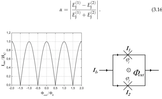
Figure 3.4: Dependence of the switching current in the SQUID loop on an
ap-plied flux in the case of symmetric junctions (α = 0). The points where the
applied flux is an integer multiple of the flux quantum are called sweet spots because they are less sensitive to flux noise. Figure obtained from [41].
The Josephson energy is given by [41]:
EJ = Φ0
2πISW. (3.17)
Due to the junction asymmetry, the circulating supercurrent induced by the external magnetic flux never reaches the critical current IC and so
22
3.5 Flux control of qubit frequencies 23
the minimum of the modulated ISW is not zero as in the symmetric case.
Therefore, the transmon has two sweet spots, where it is less sensitive to dephasing, atEmaxJ = EJ(1) +EJ(2) and at EminJ = EJ(1) −EJ(2). As shown in figure 3.5, we can move from one sweet spot to the other by applying a magnetic fluxΦext =Φ0/2.
−1 −0.5 0 0.5 1
4 4.5 5 5.5 6 6.5
Transmon frequency (GHz)
Flux (Φ / Φ
0)
ω
r
ω
d
ω
q
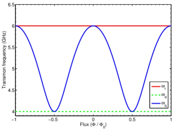
Figure 3.5: Envisaged design of qubit and resonator frequencies. The qubit frequency (—) has two sweet spots: one close to the resonator frequency (—) for the Jaynes-Cummings step, and the other resonant to the frequency of the drive (- - -) for the bit flip operations.
In order to eliminate qubit dephasing as much as possible in our ex-periment, we want to design a double sweet spot transmon. Therefore, for the Jaynes-Cummings evolution part there will be no applied flux such that the qubit frequency stays in the upper sweet spot, where it interacts strongly with the cavity. For the bit flip operations we will apply a Φ0/2
flux pulse which detunes the qubit frequency to the bottom sweet spot, where it is resonant with the frequency of the drive.
In order to implement this numerically, we first write the transmon Hamiltonian [Eq. (2.3)] in the basis of the Cooper-pair number operator
ˆ n[42]
Htransmon=4EC
∑
n(nˆ−ng)2|nihn| −
EJ
2
∑
n |nihn+1|+|n+1ihn|. (3.18)24 Numerical model description
This implementation offers us exact control of the transmon level fre-quencies given the charging energy of the transmon and Josephson ener-gies of the junctions. More importantly, it offers the possibility of mod-elling any effects that might be manifested to the flux pulses due to the electronic setup, as we shall see in the next chapter.
Figure 3.6: Sequence of two Trotter steps for the digital quantum simulation
of the Rabi model. For the Jaynes-Cummings part of the simulation, the qubit
interacts strongly with the resonator. The qubit is detuned with aΦ0/2flux pulse and a resonant driving pulse is applied, which flips the state of the qubit. The Trotter step is completed with a second Jaynes-Cummings and a bit flip operation.
3.6
Trotter step description
In the previous sections we have introduced all the elements necessary for numerically simulating the digital quantum simulation of the Rabi model proposed in 2.3.2, in a circuit QED architecture. As shown in figure 3.6, a Trotter step consists of a Jaynes-Cummings evolution part followed by an anti-Jaynes-Cummings part.
The Jaynes-Cummings evolution is described by:
HJC(1) =h¯
∑
j ∆(1)
j |jihj|+¯h∆ra
†a+hg¯ a†c+ac†, (3.19)
with∆r =ωr−ωr f, ∆(1)q =ωq(1)−ωr f.
The anti-Jaynes-Cummings evolution part consists of a Jaynes-Cummings for∆t = tJC (possibly with different qubit frequency) sandwiched by two
24
3.6 Trotter step description 25
Rxˆ,π rotations (bit flips):
UA-JC =Rxˆ,π UJC Rxˆ,π.
The Rxˆ,π rotations are implemented via a driving term, as discussed
in section 3.4, and have a finite duration tdrive ∼ 10 ns as in the
experi-ment. The free energy evolution of the photon field in the resonator state needs to be taken into account during that time, therefore the Hamiltonian describing the system during the bit flip operation is:
Hdrive =¯h∆ra†a+h¯
Ω(t)c†ei(ωr f−iωd)t+Ω∗(t)ce−i(ωr f−iωd)t
. (3.20)
Each Trotter step has, therefore, a finite time duration
τ =2(tdrive+tJC),
and the simulated Rabi model time after each step is tRabi = tJC. Notice
that due to free evolution in the cavity state during the bit flips, we no longer haveωRr =2∆r butωrR =∆r(τ/tJC). Therefore, a quantum
simula-tion in all parameter regimes can be achieved by choosing the appropriate parameters such that
ωrR =∆r(τ/tJC), ωqR=ω(1)−ω(2), gR =g.
In figure 3.7 we show the numerical evolution of the qubit and cavity states for three consecutive Trotter steps. We solve the master equation for the Hamiltonian describing the real time dynamics of the joint system:
H =¯h
∑
j
∆j|jihj|+h¯∆ra†a+¯hg
a†c+ac†
+¯h
2
Ωx(t) +iβΩ˙ x(t)ei(ωr f−ωd)tc†+Ωx(t)−iβΩ˙ x(t)e−i(ωr f−ωd)tc
, (3.21)
where Ωx(t) = ΩAmpexp
h
−(µ−t)2
2σ2
i
and ΩAmp = 0 during the
Jaynes-Cummings evolution part. We consider realistic pulses withσ=2 ns and 5σwidth.
We plot the mean photon number inside the resonator,ha†ai =Tr
ρra†a,
as well as the transmon occupation probabilities for the ground(hg|ρq|gi)
and first excited (he|ρq|ei) states. The reduced density matrices of the
qubit and the resonator
26 Numerical model description
0 0.5 1 1.5 2 2.5 3
0 0.5 1
Qubit level populations
Trotter steps
0 0.5 1 1.5 2 2.5 3
0 0.2 0.4
Average cavity photon number
Trotter steps 1st level
2nd level
Figure 3.7: Quantum simulation of Rabi model dynamics after three Trotter
steps. The ideal Rabi model dynamics (- - -) of the qubit levels (top) and cavity
photon number (bottom) are compared with the quantum simulation results at the end of each Trotter step (•). Real time evolution of the dynamics (—) shows collapses and revivals of the qubit population as expected.
are obtained from the partial trace of the joint density matrix over the qubit and resonator system, respectively.
The predictions of the Rabi model unitary evolution (described byρR) are compared to the real time dynamics of the quantum simulation after each Trotter step. As a measure of how close the two systems we calculate the fidelity[43]
F(ρ,ρR) =
Tr
q√
ρρR√ρ
2
, (3.22)
which ranges from 0, when there is no connection between them, to 1, whenρ=ρR.
26
Chapter
4
Numerical results
4.1
Simulations for ideal two-level qubits
4.1.1
Testing the limits
We first examine whether a quantum simulation of DSC Rabi model dy-namics(ωRq = 0, ωRr = gR)can be achieved in a system described by the Jaynes-Cummings model, assuming a perfect two level qubit coupled to a resonator with a typical cQED coupling strength ofg/2π =80 MHz, as proposed in [23].
0 0.2 0.4 0.6 0.8 1
0 1 2 3 4
Mean photon number
Oscillation period
Ideal Rabi dt=5 ns dt=2 ns dt=1 ns
0 1 2 3 4 5
0 0.2 0.4 0.6 0.8 1
Error per step
Trotter steps dt=2 ns
dt=1 ns dt=0.5 ns
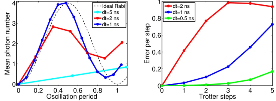
Figure 4.1:Numerically modelling the digital quantum simulation of an
effec-tive Rabi model with(ωRq = 0,ωrR = gR), for several time stepstJC, assuming
a two-level qubit strongly coupled to a resonator with g/2π = 80 MHz, as in
typical circuit QED setups. (left) Mean photon number in the resonator (-•-)
28 Numerical results
We try decreasing the time step(tJC), in order to reduce the Trotter
er-ror, until a good agreement to the ideal dynamics is achieved, for at least one oscillation period (t = 1/gR). As shown in figure 4.1, this would require implementing time stepstJC . 1 ns. However, this would be
im-possible to achieve in the lab as it goes beyond the resolution limit set by current electronics used to control circuit QED experiments.
4.1.2
Finite time Trotter steps: Slowing down the dynamics
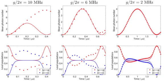
As we have seen in the previous section, a digital quantum simulation of the Rabi model in circuit QED would be impossible to implement for typical coupling strengths. Here, we present a different approach, i.e. to keep the Trotter step time fixed at a realistic value that can be achieved in the lab and vary the coupling strength g. The idea is that by lowering the coupling strength, we effectively ”slow down” the dynamics of the Jaynes-Cummings evolution. The expectation is that for finite time steps this will result in decreasing the Trotter error.
Figure 4.2:Numerically modelling the digital quantum simulation of the DSC
Rabi model(ωRq = 0,ωrR = gR)for different coupling strengths using a finite
time Trotter step ofτ = 40 ns. The plots show simulated (•) vs ideal (—) mean
photon number (top) and qubit level populations (bottom), after each Trotter step. Better agreement is observed for lower coupling strengths.
We use realistic finite time gates for the Jaynes-Cummings and bit flip parts, tJC = tdrive = 10 ns. A Trotter step, therefore, requires τ = 40 ns
28
4.1 Simulations for ideal two-level qubits 29
of experimental time and corresponds to 10 ns of ideal Rabi evolution dy-namics, which we rescale accordingly for the purposes of demonstration. Using the digital approximation
eiHRt = (eiH (1)
JCt/neiH
(2)
A-JCt/n)n+ [H(1)
JC ,H (2) A-JC]
t2
2n +O(t
3)
, (4.1)
we want to simulate Rabi model dynamics in the deep-strong coupling (DSC) regime for the simple case whereωRq =0, ωrR= gR.
In order to reduce the Trotter error, we set the rotating frame at the qubit frequency during the Jaynes-Cummings steps,
ω1q =ω2q =ωr f,
such that∆q =0, and choose the resonator frequencyωr such that
∆r =ωr−ωr f =g(tJC/τ) = g/4.
As shown in figure 4.2, good agreement can be achieved even for one period of Rabi model dynamics (gRt = 1), however for unusually low coupling strengths, below 10 MHz. The price that one has to pay when going to lower coupling strengths is that the experimental time should be extended and the fidelity of the simulation is going to be limited by decoherence mechanisms. We will examine this effect in section 4.2.2.
4.1.3
Eliminating first order Trotter errors
In the Trotter sequence of (4.1), the first order Trotter error is proportional to
∑
i>j
[Hi,Hj] = [HJC(1),HA-JC(2) ]. (4.2)
We can reduce this error by setting the rotating frame to the qubit fre-quency, as in the simulations of the previous section, however, due to the finiteness of the bit flip operation we cannot eliminate it completely.
An alternative, is to try a symmetric implementation of the Trotter step:
eiHRt '
eiH (1)
JCt/2neiH
(2)
A-JCt/neiH
(1)
JCt/2n
n
, (4.3)
i.e. apply the Jaynes-Cummings partH(1)JCfor half of the time tJC
2 , then
the anti-Jaynes-Cummings part (as before) and finally anotherH(1)JC for tJC
30 Numerical results
In this case, the first order Trotter error
∑
i>j
[Hi,Hj]
t2 2n =
HJC
2 ,HA-JC
+
HA-JC,
HJC
2
t2
2n (4.4)
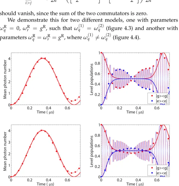
should vanish, since the sum of the two commutators is zero.
We demonstrate this for two different models, one with parameters
ωRq = 0, ωRr = gR, such that ω (1)
q = ωq(2) (figure 4.3) and another with
parametersωqR =ωRr = gR, whereω (1)
q 6=ω(2)q (figure 4.4).
Figure 4.3:Numerically modelling the digital quantum simulation of an
effec-tive Rabi model interaction withωRq =0, ωRr = gR.
Model parameters: qubit frequenciesω(q1)/2π = ω(q2)/2π = 6GHz; resonator
frequencyωr/2π=6.0015GHz; couplingg/2π=6MHz.
The plots show simulated (-•-) vs ideal (—) average cavity photon number (top) and qubit level populations (bottom). Simulations for non-symmetric Trotter step (left) are compared to the symmetric case (right).
30
4.1 Simulations for ideal two-level qubits 31
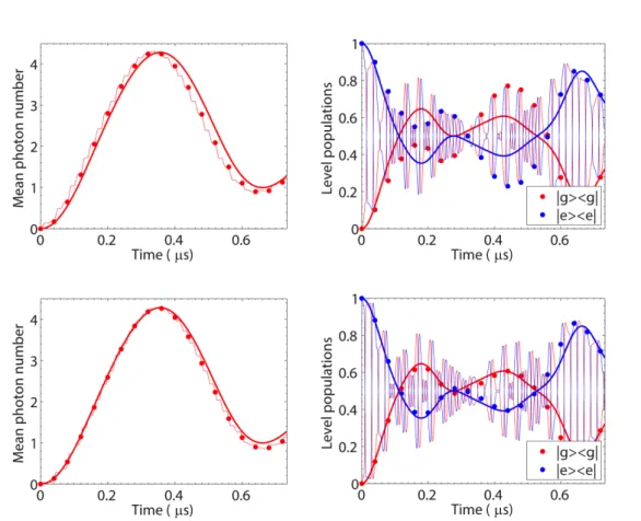
Figure 4.4:Numerically modelling the digital quantum simulation of an
effec-tive Rabi model interaction withωRq =ωRr = gR.
Model parameters: qubit frequenciesωq(1)/2π = 6GHz, ωq(2)/2π = 5.994GHz;
resonator frequencyωr/2π=6.0015GHz; couplingg/2π =6MHz.
The plots show simulated (-•-) vs ideal (—) average cavity photon number (top) and qubit level populations (bottom). Simulations for non-symmetric Trotter step (left) are compared to the symmetric case (right).
At first, we notice that the effect of eliminating the first order Trotter error is more drastic in the second case, where∆q 6=0, and it is manifested
predominantly in the qubit level population plots. Looking at the plots more carefully, we realise that the envelopes of the real time dynamics are the same in both cases, with a relative shift. Therefore, from the experi-mentalist’s point of view, first order Trotter errors are eliminated simply by measuring the qubit and resonator states at different times.
32 Numerical results
Figure 4.5: Symmetric vs non-symmetric implementation of the Trotter step. Fidelity of the quantum simulation to the ideal Rabi model dynamics with pa-rametersωRq = ωrR = gR(left) andωRq = 0,ωRr = gR(right).
4.1.4
Simulations for various coupling strengths
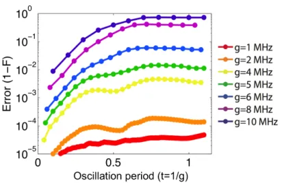
Having eliminated first order Trotter errors, we model a number of quan-tum simulations for a range of coupling strengths from 1 to 10 MHz. As shown in figure 4.6, it is possible to reduce the Trotter error by several orders of magnitude by decreasing the coupling strength.
Figure 4.6: Trotter error evolution for a range of coupling strengths in a digital quantum simulation of an effective Rabi model with parameters
ωRq = 0, ωrR = gR.
32
4.2 Simulations for a realistic circuit QED setup 33
4.2
Simulations for a realistic circuit QED setup
4.2.1
From qubit to transmon - adding the third level
As a first step towards more realistic scenarios for a quantum simulation of the Rabi model using a circuit QED setup, we include the third level of the transmon. We run again the simulations of figure 4.3 for the same pa-rameters(ωqR =0, ωRr =gR), including an anharmonic qutrit with typical
transmon anharmonicities −500 MHz . α
2π . −200 MHz. In figure 4.7,
we plot the simulation results for the same parameters as in figure 4.3, using a transmon with a typical anharmonicity of -300 MHz.
0 0.1 0.2 0.3 0.4 0.5 0.6 0.7
0 0.5 1 1.5 2 2.5 3 3.5 4
Average cavity photon number
Time (us)
0 0.1 0.2 0.3 0.4 0.5 0.6 0.7 0 0.1 0.2 0.3 0.4 0.5 0.6 0.7 0.8 0.9 1
Transmon level populations
Time (us) 1st level 2nd level 3rd level
Figure 4.7:Numerically modelling the digital quantum simulation of an
effec-tive Rabi interaction with ωqR = 0, ωRr = gR, in a cQED setup using a three
level transmon. Simulated (•) vs ideal (—) average cavity photon number (left)
and transmon level populations (right) for the same parameters as in figure 4.3, including the third level (α/2π= −300MHz).
We observe that the addition of the third level has a considerable ef-fect on the simulation fidelity, despite the fact that it is not being popu-lated(. 10−5)after each Trotter step, as a result of our optimised DRAG pulses. We examine this more carefully in figure 4.8, where we compare the simulation fidelity for a range of coupling strengths using a three level transmon and varying the anharmonicity.
As expected, the simulation fidelity gets better as|α|is increased, which is practically achieved by increasing the charging energy, EC/¯h ∼ |α|.
However, as we have discussed in section 2.2, we need EJ/EC & 30 in
34 Numerical results
0 0.2 0.4 0.6 0.8 1 1.2
0 0.1 0.2 0.3 0.4 0.5 0.6 0.7 0.8 0.9 1
α/2π = −500 MHz
Fidelity Oscillation period g=2 MHz g=4 MHz g=5 MHz g=6 MHz g=8 MHz
0 0.2 0.4 0.6 0.8 1 1.2
0 0.1 0.2 0.3 0.4 0.5 0.6 0.7 0.8 0.9 1
α/2π = −400 MHz
Fidelity Oscillation period g=2 MHz g=4 MHz g=5 MHz g=6 MHz g=8 MHz
0 0.2 0.4 0.6 0.8 1 1.2
0 0.1 0.2 0.3 0.4 0.5 0.6 0.7 0.8 0.9 1
α/2π = −300 MHz
Fidelity Oscillation period g=2 MHz g=4 MHz g=5 MHz g=6 MHz g=8 MHz
0 0.2 0.4 0.6 0.8 1 1.2
0 0.1 0.2 0.3 0.4 0.5 0.6 0.7 0.8 0.9 1
α/2π = −200 MHz
Fidelity Oscillation period g=2 MHz g=4 MHz g=5 MHz g=6 MHz g=8 MHz
Figure 4.8: Fidelity plots for the quantum simulation of the DSC Rabi model
(ωRq = 0, ωRr = gR)using a three level transmon coupled to a resonator for a
range of coupling strengths and anharmonicities.
which suggests that we needEC/¯h ∼300 MHz.
From figure 4.8, we conclude that a high fidelity (90%) quantum sim-ulation is achievable for coupling strengthsg/2π .5 MHz and an anhar-monicity|α|/2π &300 MHz.
4.2.2
Dissipation
We implement dissipation mechanisms by adding the appropriate Lind-blad superoperator associated with each decay rate in the master equation (see section 3.2). The key sources of decoherence are the transmon and resonator relaxation timesT1=1/γ−,Tcav =1/κas well as the transmon
dephasing timeT2 =1/γφ.
34
4.2 Simulations for a realistic circuit QED setup 35
Comparing dissipation mechanisms
We first want to identify the most important form of dissipation. We ex-amine the case whereg/2π =4 MHz, which we have found to give high fidelities before, and study the effect of each decay mechanism on the sim-ulation fidelity. The experimental time of the simsim-ulation is∼1µs and we add one by one the relative dissipation times (of 10µs each).
0 0.2 0.4 0.6 0.8 1 0.5
0.55 0.6 0.65 0.7 0.75 0.8 0.85 0.9 0.95 1
Fidelities for different decay mechanisms (g=4 MHz)
Fidelity
Time(us) No Decay
T1=10us T2=10us Tcav=10us
Figure 4.9: Fidelity plots comparing the impact of each decay mechanism on
the quantum simulation forg/2π =4 MHz.
As shown in figure 4.9 the resonator decay is the most limiting factor, therefore, we should aim for a high quality resonator when designing the experiment.
Realistic decay rates
36 Numerical results
T2 ∼1µs. This is the price that we have to pay in order to strongly couple
a qubit and a resonator with such a low coupling strength.
−1 −0.5 0 0.5 1 4 4.5 5 5.5 6 6.5
Transmon frequency (GHz)
Flux (Φ / Φ
0) ω r ω d ω q
−1 −0.5 0 0.5 1 4 4.5 5 5.5 6 6.5
Transmon frequency (GHz)
Flux (Φ / Φ
0) ω r ω d ω q
Figure 4.10: Design of qubit and resonator frequencies. (left) Ideal frequency scheme as a function of flux. (right) Most realistic frequency scheme based on possible deviation in targeting the transmon frequencies.
In figure 4.11 we plot the fidelity of the quantum simulation for the most likely and feasible decay rates that we expect in the experiment. We aim to have a high quality factor resonator with a relaxation time of 15µs and a typical qubit with T1 = 10 µs. The dephasing time is set to be 1 µs
during the Jaynes-Cummings and 10 µs during the bit flip operation, as expected from the design in figure 4.10 (right).
0 0.2 0.4 0.6 0.8 1
0.5 0.55 0.6 0.65 0.7 0.75 0.8 0.85 0.9 0.95 1
Simulation fidelity incuding dissipation (g=4 MHz)
Fidelity Time(us) No Decay T1=10us T2=1−10us Tcav=15us Combined
Figure 4.11:Fidelity plots of the quantum simulation with realistic decay
mech-anisms forg/2π =4 MHz.
36
4.2 Simulations for a realistic circuit QED setup 37
4.2.3
Finite-bandwidth flux control: RC filter
In our numerical model, the transmon frequencies can be tuned by ap-plying square flux pulsesΦext from 0 toΦ0/2 and then diagonalising the
transmon Hamiltonian (see section 3.5). This implementation allows us to model bandwidth limited flux pulsing, naturally arising from our elec-tronics setup.
In an experimental situation, the applied voltage that induces the flux pulses to the SQUID loop, is attenuated due to the microwave electronics. This effect can be simulated as a single pole low pass filter with a cut-off frequency fcut = 2π1RC, where RC is the time constant of the filter.
There-fore, any input voltageVinis modified asVout = 1+jVωinRC, in the frequency
domain.
As a result, the response of the flux bias line is slowed down and the flux pulse will no longer be a step function. In order to model this effect numerically, we calculate the response in the time domain, by taking the Laplace transform of the transfer function 1+j1ωRC. Therefore, an applied square flux pulse is modified as
Φout =Φin
e−t/RC
RC . (4.5)
0 5 10 15 20 25
0.5 0.55 0.6 0.65 0.7 0.75 0.8 0.85 0.9 0.95 1
Simulation fidelity for filtered flux pulses (g=4 MHz)
Fidelity
Trotter steps
No filter RC filter
Figure 4.12:Impact of a single pole low-pass filter of RC=1.25 ns in the simula-tion fidelity.
38 Numerical results
4.2.4
Final real-world quantum simulations
In figure 4.13, we show that an analog-digital quantum simulation of the Rabi model in a realistic circuit QED setup with a three-level transmon coupled to a resonator, is feasible with a good fidelity including experi-mental parameters such as finite time pulses, bit flips implemented via op-timised DRAG pulses, bandwidth-limited flux pulsing for qubit frequency detuning between Trotter steps, as well as cavity and transmon relaxation and dephasing processes.
Figure 4.13: Numerically modelling the digital quantum simulation of an
ef-fective Rabi interaction with ωqR = 0, ωrR = gR. Model parameters:
qubit-cavity detuning = 1 MHz; coupling 2gπ = 4 MHz; transmon anharmonicity
α
2π ' −300MHz; photon decay timeTc = 30µs; transmon relaxationT1= 10µs
and dephasingT2 =1 − 10µs. The plots on the top show simulated (•) and ideal
(—) transmon level populations (left) and average cavity photon number (right). Fidelity of the simulated system state to the ideal state after each Trotter step is plotted on the bottom.
38
4.3 Exploring the dynamics of the deep-strong coupling regime 39
4.3
Exploring the dynamics of the deep-strong
coupling regime
In this section, we explore the dynamics of the Rabi model in regimes be-yond ultra-strong coupling. We show that deep-strong coupling (DSC) provides extraordinary dynamics exhibiting special types of hybrid en-tanglement between the qubit and macroscopic Schr ¨odinger cat states. We identify the Wigner function as a key tool in probing these dynamics, and we demonstrate that they can be reproduced with the digital quantum simulations scheme discussed so far.
4.3.1
Strong coupling and beyond
The Jaynes-Cummings regime
As we have previously discussed, the strong coupling regime of the Rabi model, whengR ωRq,ωRr, is described by the Jaynes-Cummings model of equation (2.2). In the absence of non-conserving excitation terms, it is obvious that nothing happens when we start without any excitation in the system (|gi|0i). When an excitation is added to the system, e.g. the qubit initially in the excited state |ei, we observe the well-known Rabi oscillations|ei|0i ↔ |gi|1i that lead to a highly entangled superposition between the qubit and a photon Fock state:
1
√
2(|0i|ei+|1i|gi). (4.6)
Parity chains
As the coupling strength becomes comparable to the qubit and cavity fre-quencies, the RWA breaks down and the counter-rotating termsσ+a†, σ−a of the Rabi Hamiltonian [Eq. (2.1)] become dominant. The dynamics can be described in the Hilbert space by two unconnected parity chains de-pending on the initial state [7]:
|gi|0i ↔ |ei|1i ↔ |gi|2i ↔ |ei|3i ↔ |gi|4i. . . (p= +1), (4.7)
|ei|0i ↔ |gi|1i ↔ |ei|2i ↔ |gi|3i ↔ |ei|4i. . . (p=−1), (4.8)
where pis the eigenvalue of the parity operator:Π =σz (−1)a†a.
non-40 Numerical results
Figure 4.14: Rabi model energy level structure (left) and evolution of
dy-namics in Hilbert space (right). The blue arrows indicate interactions via the
energy-conserving termsσ+a, σ−a† while the red arrows stand for interactions
via the counter rotating terms σ+a†, σ−a. The latter are absent in the
Jaynes-Cummings regime and the Hilbert space is restricted to excitation concerving Jaynes-Cummings doublets.
conserving excitations terms break into the Jaynes-Cummings doublets that we discussed before.
4.3.2
Superpositions of coherent states
We now examine more carefully the DSC regime of the Rabi model in the simple case that we mostly discussed in the previous chapter, with pa-rameters: gR = ωR, ωqR = 0. As we have already observed (figure 4.13
for example), even when starting without any excitation in the system, the mean photon number oscillates in a coherent way between zero and
ha†ai = 4, i.e. the system evolves via the first parity chain(p= +1). In order to better understand these dynamics we look at the evolution in phase space, which contains more information than just the evolution of the photon number. We, therefore, reconstruct the Wigner quasiproba-bility distribution of the cavity state which is defined as [44]
W(α) = 2 π
∞
∑
n=0
(−1)nhn|D−1(α)ρrD(α)|ni. (4.9)
D(α) = exp[αa†−α∗a] is the displacement operator of the mode. It is also defined byD(α)|0i =|αi, i.e. when acting on the vacuum it creates a
coherent state |αi = e−
|α|2
2 ∑∞n=0√αn
n!|ni. In general, D(α)displaces a
pho-40
4.3 Exploring the dynamics of the deep-strong coupling regime 41
ton state in phase space by a magnitude and direction set by the complex numberα.
Looking at the Wigner function of the cavity state, allows us to extract very interesting information about the photon field and its evolution in phase space. A remarkable feature about this function is that it becomes negative for non-classical states such as Fock or Schr ¨odinger cat states, and has therefore been proposed as a measure of the non-classicality of states [45].
Re(α)
Im(
α
)
−4 −2 0 2 4
−4 −2 0 2 4 0 0.2 0.4 0.6
Re(α)
Im(
α
)
−4 −2 0 2 4
−4 −2 0 2 4 0 0.1 0.2 0.3
Re(α)
Im(
α
)
−4 −2 0 2 4
−4 −2 0 2 4 0 0.1 0.2 0.3 0 0.1 0.2 0.3 Cavity Wigner function evolution
Re(α)
Im(
α
)
−4 −2 0 2 4
−4 −2 0 2 4
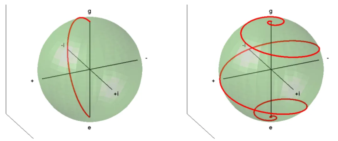
Figure 4.15: Evolution of the Wigner function in the DSC regime of the Rabi
model with parameters gR = ωR, ωR
q = 0. The cavity initially in the
vac-uum state (top left) turns into a supposition of two coherent states|αiand| −αi
with α = 2 (top right). This point corresponds to a photon number peak at
ha†ai = |α|2 = 4.
In figure 4.15, we plot the evolution of the Wigner function of the cavity in phase space for the DSC Rabi model with gR = ωR, ωqR = 0, for half
42 Numerical results
and| −αiwithα =2.
In order to understand this evolution we look at the interaction term in the Rabi Hamiltonian,
HI =hg¯ Rσx
ae−iωrt+a†eiωrt. (4.10)
The cavity density matrix evolves asU†IρrUI, where
UI =exp
−i
Z t
0 dτ g R
σx
ae−iωrτ+a†eiωrτ
=exp
σx
Z t
0 dτ(−ig
R)eiωrτ
a†−
Z t
0 dτ (ig
R)e−iωrτ
a
.
(4.11)
This interaction is, therefore, equivalent to a time-dependent displacement operation on the cavityD(α) = exp[αa†−α∗a], that is determined by the complex number α = R0tdτ (−igR)eiωrτ and depends on the qubit state (σxoperator).
For example, if the qubit is initially in an eigenstate ofσxand the cavity
in the vacuum state, this will result in the creation of a coherent state, as: σxD(α)|±i|0i → |±i| ∓αi.
Maximum displacement
We can calculate the modulus of the cavity displacement
|α|=|igR
Z t
0 dτ e iωrτ|
= g
R
ωr
|eiωrt−i|
= g
R
ωr q
cos2ω
rt+ (sinωrt−1)2
= g
R
ωr √
2−2 cosωrt. (4.12)
Att= π
ωr the displacement reaches its maximum value:
|α|max= 2
gR
ωr . (4.13)
Therefore, the size of these coherent states, and the quantum superpo-sition, increases as we increase the coupling strength relatively to the nat-ural frequencies in the system. Notice that in the strong coupling regime,
42
4.3 Exploring the dynamics of the deep-strong coupling regime 43
gR ωrR, there is no cavity displacement because the cavity terms rotate much faster than the coupling strength.
4.3.3
Hybrid discrete - continuous variable entanglement
For a better understanding of the photon-qubit dynamics, we first calcu-late the negativity of the joint system, which is defined as the absolute value of the sum of negative eigenvalues of the partial transpose of the system density matrixρT [46]
N(ρ) =
∑
i
|λi| −λi. (4.14)
This quantity vanishes for states which are not entangled [47].
0 0.2 0.4 0.6 0.8 1
0 0.2 0.4 0.6 0.8 1
Qubit−Cavity Negativity
Time*g 0 0.2 0.4 0.6 0.8 1
0 1 2 3 4
Mean photon number
Time*g
Figure 4.16: Negativity of the qubit-cavity in the Rabi model with parameters
gR = ωR, ωR
q = 0 (left) and corresponding mean photon number evolution
(right).
From figure 4.16, we verify the existence of entanglement in the system, however in order to verify its nature we need to look at the state in the cavity after conditioning on different qubit bases.
The cavity density matrix after conditioning on the qubit being in a certain state|ψqiis
ρcondr =Trqρ(|ψqihψq| ⊗I), (4.15)
which experimentally amounts to measuring the qubit in|ψqi.
![Figure 2.1: Schematic of a two-level atom coupled to a quantised oscillator mode. Figure obtained from [27]](https://thumb-us.123doks.com/thumbv2/123dok_us/8268474.2190243/12.892.311.645.200.484/figure-schematic-level-coupled-quantised-oscillator-figure-obtained.webp)