PRIORITY SCHEDULING OF JOBS WITH HIDDEN TYPES
Zhankun Sun
A dissertation submitted to the faculty of the University of North Carolina at Chapel Hill in partial fulfillment of the requirements for the degree of Doctor of Philosophy in the Department of Statistics
and Operations Research.
Chapel Hill 2014
c
2014
ABSTRACT
ZHANKUN SUN: PRIORITY SCHEDULING OF JOBS WITH HIDDEN TYPES. (Under the direction of Nilay Tanık Argon and Serhan Ziya.)
In service systems, prioritization with respect to the relative “importance” of jobs helps allocate the limited resources efficiently. However, the information that is crucial to determine the importance level of a job may not be available immediately, but can be revealed through some preliminary in-vestigation. While investigation provides useful information, it also delays the provision of services. Therefore, it is not clear if and when such an investigation should be carried out. To provide insights into this question, we consider a service system with a single server and the two possible types of jobs, where each type is characterized by its waiting cost and expected service time. Jobs’ type identities are initially unknown, but the service provider has the option to spend time on investigation to deter-mine the type of a job albeit with a possibility of making an incorrect determination. Our objective is to identify policies that balance the time spent on information extraction with the time spent on service. In this dissertation we consider two settings: one with finitely many jobs present at time zero and no external arrivals; the other with exogenous arrivals.
When there are external arrivals to the system, we show that the optimal dynamic policy is of threshold type. The structure of the optimal policy implies that when there are few less-important jobs waiting for service, the server should perform investigation; otherwise, the server should stop inves-tigation and serve jobs directly. Given that it is almost impossible to obtain an analytical expression of the threshold, we develop a heuristic policy based on the results for the clearing system. We carry out a simulation study and find that the heuristic policy performs significantly better than No-Triage Policy in most cases; for the rest, it performs at least as well as No-Triage Policy.
ACKNOWLEDGMENTS
TABLE OF CONTENTS
LIST OF TABLES . . . viii
LIST OF FIGURES . . . ix
1 INTRODUCTION . . . 1
2 LITERATURE REVIEW . . . 5
2.1 Priority scheduling with perfect information . . . 5
2.2 Priority scheduling with imperfect information . . . 7
3 PRIORITY SCHEDULING OF JOBS WITH HIDDEN TYPES IN A CLEARING SYSTEM . . . 10
3.1 Introduction . . . 10
3.2 Model description . . . 11
3.3 Benchmark policies . . . 12
3.3.1 Comparison of benchmark policies . . . 13
3.3.2 Insights from comparison of policiesT P1andT P2 . . . 17
3.3.3 Better triage better outcome? . . . 19
3.4 State-dependent policies . . . 20
3.4.1 Markov decision process formulation . . . 20
3.4.2 Complete characterization of the optimal policy . . . 21
3.5 Numerical study: performance comparison of the proposed policies under linear and non-linear waiting costs . . . 24
3.5.1 Performance comparison when waiting costs are linear in time . . . 25
4 PRIORITY SCHEDULING OF JOBS WITH HIDDEN TYPES IN A
QUEUEING SYSTEM . . . 32
4.1 Introduction . . . 32
4.2 Model description . . . 32
4.3 State-dependent policies . . . 34
4.3.1 Markov decision process formulation . . . 34
4.3.2 Characterization of the optimal policy . . . 35
4.3.3 Proof of Theorem 4.3.1 and Proposition 4.3.2 . . . 37
4.4 Simulation study . . . 41
5 EXTENSIONS . . . 44
5.1 Multiple identical servers . . . 44
5.2 Instantaneous triage . . . 45
5.2.1 Threshold-type policies . . . 49
5.3 When triage is not optional . . . 52
6 CONCLUSIONS AND DIRECTIONS FOR FUTURE RESEARCH . . . 55
APPENDIX A PROOF OF RESULTS IN CHAPTER 3. . . 58
APPENDIX B PROOF OF RESULTS IN CHAPTER 4. . . 79
APPENDIX C PROOF OF RESULTS IN CHAPTER 5. . . 110
LIST OF TABLES
3.1 Notation used in writing optimality equations in a compact form. . . 21 3.2 95% confidence intervals for the mean and maximum percentage
improvement in the total expected cost by using the optimal policy as
opposed to benchmark policies. . . 25 3.3 Performance comparison for the convex cost case - 95% confidence
interval for the mean percentage increase in total expected cost when
compared with that under the optimal policy. . . 29 3.4 Performance comparison for the S-shaped cost case - 95% confidence
interval for the mean percentage increase in total expected cost when
compared with that under the optimal policy. . . 30 3.5 Performance comparison for the concave cost case - 95% confidence
interval for the mean percentage increase in total expected cost when
compared with that under the optimal policy. . . 31
4.1 Comparison in the average cost by using the heuristic policyT has
LIST OF FIGURES
3.1 Comparison of Triage-Prioritize-Class-1 (T P1) and No-Triage (N T)
policies. (u= 0.15, v1 = 0.95, v2 = 0.95, τ1= 1, τ2 = 3, N= 100). . . 15 3.2 Comparison of Triage-Prioritize-Class-1 (T P1) and No-Triage (N T)
policies, different levels ofη. . . 16 3.3 Visual description of the optimal policy whenk1 = 0andh1= 10,
h2 = 1, τ1 = 1, τ2 = 2, v1= 1, v2 = 0.95, u= 0.26, p= 0.8, N = 18. . . 23 3.4 The waiting cost functions assumed in the numerical study. . . 28
4.1 Visual description of the optimal policy whenk1 = 0andλ= 0.6,
h1 = 10, h2 = 1, τ1 =τ2 = 1, v1 = 0.9, v2 = 0.95, u= 0.25, p= 0.6.. . . 36
5.1 An example of the threshold-type policy when triage is instantaneous
CHAPTER 1: INTRODUCTION
In service systems, first-come-first-serve is a frequently used service discipline, however, in reality there are many situations of practical interest where customers are served not in the order of their arrival but according to the priorities that are assigned based on their relative “importance.” In this dissertation, we refer this type of service aspriority scheduling. Priority scheduling is prevalent in service systems. Especially when service capacity is limited, prioritization helps allocate this limited resource in a way that aligns with the overall objectives of the service provider. Priority scheduling has been practically applied in call centers, banks, machine maintenance, Emergency Departments (ED) of hospitals, military communications, etc. For example, in the EDs, the patients who need immediate medical attention will be seen first if the existing patients can be delayed.
Priority scheduling requires information about the jobs (we use jobs to denote customers, ma-chines, parts, patients, etc.) to assign them priorities. This information is sometimes immediately available and can be used to determine priority levels. For example, a service provider who is inter-ested in providing priority service to its “good” customers, might be able to use past data to determine its customers’ priority classes instantly as they arrive. In some cases, however, the information that is crucial to determine the priority level of a job is not available immediately but can be obtained with some investigation. This investigation produces useful information but at the expense of delaying the service process. It is not clear if and when engaging in such investigation justifies the extra delay imposed. The goal of this research is to shed some light on this question.
Specific examples will help illustrate the practical relevance of the information/delay trade-off described above. When healthcare resources are severely restricted in comparison with the urgent demand as in the case of mass-casualty incidents (MCI)1or clinics in rural areas and underdeveloped countries, patients go through a process called “triage” before they are given treatment. The objective of triage is to determine the seriousness of the patients’ conditions and prioritize them accordingly. 1
When on-site medical personnel is not very limited in numbers, triage and treatment can proceed simultaneously and therefore unless triage takes unusually long it does not typically lead to delays in treatment or transportation. However, in austere mass-casualty conditions, battlefields, and clinics in economically deprived areas where in some cases healthcare services are delivered through mobile clinics, a single person or a team can be in charge, which necessitate a careful balancing of time spent on triage and time spent on treatment or a more thorough examination of the patients. The information/delay trade-off also appears in other contexts, such as prioritization of requests submitted daily to internal maintenance and repair departments (Taghipour et al., 2011); prioritization of sales leads in marketing particularly in business-to-business settings (Lichtenthal et al., 1989; Wilson, 2003; D’Haen and den Poel, 2013), where time is invested to assess the likelihood of existing leads to be successfully converted to actual sales; and intelligence (particularly human intelligence) collection management (Kaplan, 2010, 2012; Ni et al., 2013), where agents make some initial investigation of existing ambiguous cues, which might possibly be pointing to potential terrorist activities, and prioritize them prior to more in-depth investigation.
Despite the fact that these examples arise in very different contexts they share some key features: jobs are heterogeneous regarding their “importance” (or “urgency”) and possibly their service require-ment. The decision maker knows that the jobs are heterogenous but there is no information readily available, which can help in distinguishing one job from another. Investigating any given job reveals some information for that job, which then can be used to determine whether or not the job should get a priority in service but this information can be noisy and thus may lead to an incorrect classifica-tion. Furthermore, the investigation is “costly” in the sense that it takes time and resources. Spending time in investigation essentially eats away from the time that can be spent in actually serving the jobs. Thus, in all these examples, the fundamental goal is to carefully balance the time spent on information extraction with the time spent on serving the jobs.
In this thesis, we aim to contribute to the understanding of this trade-off and provide insights on how the decision on investigation should be made in order to achieve such a balance. The goal is to develop a generic formulation whose analysis leads to insights into how that can be done, rather than to model any single one of the application contexts mentioned above with its unique features.
can serve a job without knowing its type. Alternatively, the server can triage a job, place the job in a particular class, which correlates with the type of the job, and then either proceed to serve that job right away or put that job aside for awhile in order to serve later. (We borrow the medical terminology “triage” to refer to the investigative process which results in the classification of jobs.) Triage is imperfect meaning that jobs can be classified incorrectly. The type of a job determines the expected service time for that job and the “cost” of keeping the job waiting. The objective is to minimize the total expected cost or the long-run average cost, depending on the specific model settings.
The remainder of this thesis is organized as follows. Chapter 2 reviews the literature on job scheduling problems and discuss how this work will contribute to the literature. Chapter 3 presents the description and analysis of our clearing model2 . We first compare four simple policies and the analysis leads to some seemingly counter-intuitive findings. Then we provide a complete characteriza-tion of the optimal dynamic policy. In particular, we find that there is a switching curve that separates the states in which triage should be performed from the others. One interesting insight that comes out of this characterization is that spending time on triage helps if there are sufficiently many jobs but not when there are relatively few. Our analytical results assume that waiting cost is a linear function of time. A numerical study reveals that even though the structure of the optimal policy can be different when the waiting cost function is not linear, the heuristic policies developed based on the results in our model with linearity assumption perform well.
In Chapter 4, we study the information/delay trade-off in a setting where there are external arrivals to the system. With the assumption of a Poisson arrival stream and independent and identical (i.i.d) exponential service times, we show that the optimal policy on whether to triage or not in order to minimize the long-run average cost is characterized by a switching curve. To prove the structure of the optimal policy, we show various properties of the optimal value functions of a corresponding model with discounting, then extend these results to the optimal bias functions in our original model. With a simulation study, we observe that a heuristic policy of threshold type can improve significantly over the policy of skipping triage all the time.
In Chapter 5, we study three extensions to the models in Chapters 3 and 4. In Section 5.1, we study a clearing model with multiple identical servers instead of a single server. In Section 5.2, we 2
consider a model where there are external arrivals and triage is instantaneous but incurs a fixed cost. In Section 5.3, we analyze the case where triage is required for service, in which case the decision is to determine the class to be prioritized after triage: an untriaged job, or a job that is classified as class-1 or class-2. In each section, we describe the model assumptions and provide partial or complete characterization of the optimal policy.
CHAPTER 2: LITERATURE REVIEW
There are two streams of papers that are relevant to our work: (i) traditional job scheduling and (ii) priority scheduling under imperfect information on job identities.
2.1 Priority scheduling with perfect information
Within the context of this dissertation, job scheduling is the process of determining the order ac-cording to which jobs of different types will be processed. There are many different versions of the job scheduling problem. For example, a clearing system versus a system with exogenous arrivals, a single-server system versus a multi-server system, deterministic settings versus stochastic environ-ments, preemption versus non-preemption, linear cost versus nonlinear cost, etc. There can be also different objectives, depending on the settings of the specific job scheduling problem, such as mini-mizing the total (or average) waiting time (or cost), minimini-mizing the total tardiness or the number of tardy jobs, etc. There exists substantive work on job scheduling problems. Pinedo (2008) provides an extensive review of the scheduling problems that have been studied. We here review only the most related work that establish the optimality of thecµrule under various conditions.
There are several papers that prove the optimality of thecµrule in settings where there is no exter-nal arrival. Smith (1956) studies a single-stage production system with deterministic processing times and identical release times for all jobs. Thecµrule is shown to be optimal to minimize the weighted sum of job completion times. Since then, thecµrule and its various generalizations are shown to be optimal in models with different settings. Pinedo (1983) considers the stochastic counterpart of the above model where the processing time of jobj is exponentially distributed with rateλj and the re-lease time is a random variable with arbitrary distribution. Preemption is allowed. The author showed that it is optimal to process the job with the highest value ofcjλj among those available.
cost and service is non-preemptive. Kakalik and Little (1971) shows that the optimality of thecµ rule holds in the larger class of state-dependent dynamic policies as well, regardless of the option of idling the server. Klimov (1974) extends the optimality of thecµrule to a multiclassM/G/1queue with feedback. Harrison (1975) considers a multiclassM/G/1system with discounted holding costs and shows that a static priority rule is optimal. Tcha and Pliska (1977) studies a model that combines discounting and feedback, and show that a static priority rule is optimal. Hirayama et al. (1989) studies a discrete-timeG/G/1queue with two classes under non-preemptive service discipline. Thecµrule is shown to be optimal to minimize the total holding cost in a finite-horizon scheduling period if the service times have a decreasing failure rate (DFR). Nain (1989) extends the optimality of thecµrule to a multiclassG/M/1queue with or without feedback. The paper also considers twoG/M/1queues in tandem and shows that thecµrule is optimal for the second queue in that it minimizes the discounted holding cost. In the single-machine scheduling with arbitrary arrivals and machine breakdowns under a preemptive-resume discipline, Righter (1994) shows that processing jobs according to the non-increasing order ofωµvalue maximizes the number of correctly completed jobs by any timetwhen processing times have a DFR andωiis the probability that jobiwill be correctly completed. Recently Budhiraja et al. (2012) studied a multiclassM(ν)/M(ν)/1model where the arrival and service rates fluctuate with a changing environment, described by the environment variableν. The authors proved that thecµrule is asymptotically optimal for minimizing an infinite-horizon discounted cost function. The papers we mentioned so far all assume linear waiting costs. Van Mieghem (1995) is the first to prove the asymptotic optimality of thecµrule in models with nonlinear costs. Specially, the model studied is aG/G/1queue with multiclass jobs and the cost incurred by a job is a convex function of the job’s sojourn time in the system. A generalized version of thecµrule, or the so called generalized-cµrule (Gcµ-rule), is shown to be asymptotically optimal in heavy traffic in that it minimizes the total cumulative delay cost for a finite time horizon. The optimality of the Gcµ-rule is robust in that it holds for a countable number of classes of jobs and several homogeneous servers. Mandelbaum and Stolyar (2004) has extended the optimality of theGcµ-rule to multiple flexible servers in parallel.
different from the above in that we consider triage together with the service process.
2.2 Priority scheduling with imperfect information
Compared with the traditional job scheduling literature, there is limited work that deal with scheduling under imperfect information on job identities. Van Der Zee and Theil (1961) appears to be the first work that considered the misclassification problem in priority queues. The authors study a single-server queue with two priority classes having expected service timesE(s1)andE(s2), respectively. Without loss of generality, assumeE(s1) < E(s2). Class 1 jobs arrive to the system according to a Poisson process with rateλ1but are misclassified into class 2 with rateδ1, class 2 jobs arrive to the system according to a Poisson process with rateλ2but are mistakenly assigned into class 1 with rateδ2. Under the assumption of misclassification, they find that prioritizing class 1 is better than FCFS in the sense of minimizing the expected waiting time if
δ1/λ1+δ2/λ2 <1. (2.1)
They also develop a fixed-priority policy where there are three priority classes and find a condition under which this policy is no worse than FCFS by approximate analysis.
While van der Zee and Theil assume that the jobs are classified and priorities are assigned auto-matically, Argon and Ziya (2009) study the problem of how to assign priorities to the jobs based on partial information on the job identities to minimize the long-run average waiting cost. The authors consider anM/G/1queue with two types of customers. The identity of each arrival is partially known in the sense that each customer brings a signal indicating the probability of being the important type. The authors show that increasing the number of priority classes decreases costs and it is optimal to give the highest priority to the customer with the highest signal. The authors also consider two-class priority policies and find the optimal cut-off level for the signal to obtain the two priority classes. The main difference of our model from theirs is that in their model the signal is free in that there is no need for triage to obtain the signal, while in our model the type identities have to be obtained through triage, perfectly or imperfectly.
unknown as well. Alizamir et al. (2012) consider a queueing model with Poisson arrivals where each customer comes from one of two types but the server does not know which type the customer belongs to. The server diagnoses each customer through a series of independent tests and classifies it based on the server’s belief. If the classification is correct, there is a reward; otherwise, there is a penalty. Each customer incurs a waiting cost during the customer’s stay in the system. The authors find the optimal policy on how many tests to do to classify an arriving customer. Our model is different from theirs in that the jobs go through a service process after classification. On the contrary, their model focuses on the diagnostic process and the server does not perform any service after classification. Dobson and Sainathan (2011) does consider the classification and service in one model. The authors compare two models and both with Poisson arrivals. In one model jobs are first sorted by a pool of homogeneous sorters and then served by another pool of homogeneous processors (so called the prioritized model) while there are no sorting in the other model (so called the base model). The main goal is to find the optimal average waiting cost for the prioritized model by appropriately setting the number of sorters and processors under an exogenous budget constraint and compare the optimal waiting cost of the prioritized model and that of the base model. They find that sorting does not always benefit the system. Our model is different since we consider for a fixed number of servers that are capable of performing both triage and service tasks. More specifically, we concentrate on control decisions that are made dynamically based on the system state whereas Dobson and Sainathan (2011) focuses on a design problem.
CHAPTER 3: PRIORITY SCHEDULING OF JOBS WITH HIDDEN TYPES IN A CLEARING SYSTEM
3.1 Introduction
In this chapter, we investigate a problem that is similar to traditional scheduling problems with some important differences. We assume there are finitely many jobs at the beginning. The exact types, characterized by the service times and hold cost rates, are unknown to the server initially, however, the server has the option to spend some time to extract these information. Thus, our focus is on settings where an unexpected event triggers the sudden appearance of a large number of jobs to take care of (as in the case of mass-casualty events which necessitate patient triage and prioritization or search and rescue operations), where jobs accumulate at the beginning of a service period, say in the morning (as in the case of patients lining up to be seen in mobile clinics), or where a certain number of tasks are assigned to a single person (for example, a salesperson or an intelligence agent) to take care of over a certain period of time. The objective is to find the optimal policy that minimize the total expected cost by assigning priorities to the jobs and making decisions on whether or not to spend time to extract the type information.
3.2 Model description
We consider a single-server clearing system in which at timet= 0there areN ≥2jobs waiting to be served. There will be no new job arrivals. Each job belongs to one of two types: type-1 or type-2. The probability of a randomly chosen job being of type 1 isp ∈ (0,1)and that of type 2 is q= 1−pindependently of all the other jobs as well as the service process. (The cases thatp= 0 or 1
are trivial and not of interest.) A job from typeiincurs a holding cost ofhi for each unit of time the job stays in the system, and the expected service time for a typeijob isτi<∞, i= 1,2, with some general distribution. We assume that the service times of all jobs are independent conditional on their types. Once the service of a job is over, it leaves the system. The objective of the service provider is to minimize the expected total waiting cost of all jobs. If the type of each job were to be known, according to the well-knowncµ-rule, the optimal policy would be to give priority to type-1 jobs if h1/τ1 ≥ h2/τ2and to type-2 jobs otherwise. However, in our problem, whilepis known, the types of jobs are unknown to the decision maker.
The server does not need to know the type of the job to serve it but s/he can choose to perform an investigative task first in an effort to learn more about the type of the job, which can be used to determine the service order. Following the medical terminology, we call this investigative tasktriage and the act of performing triageto triage. Triage time for each job is independent of everything else including the job’s type and its expected value is denoted byu <∞. As in the case of service times, we make no further assumptions on the distribution of triage times. As a result of triage, the job is classified as either class-1 or class-2. Note that thetypeof a job is an inherent characteristic unknown to the decision maker while itsclassis an attribute assigned after triage and is observed by the decision maker. Once a job is classified, the server can either proceed to serve the job immediately or simply puts it away making note of its class information, and moves on to another job. The service time of a job does not change depending on whether or not the job’s class information is available. It only depends on the type of the job.
as class-1, we say that the job ismisclassified. Letvi denote the probability of classifying a type-i job as class-iwherevi ∈ [0,1]fori = 1,2. Without loss of generality, we make the following two assumptions throughout this chapter unless otherwise stated:
Assumption 3.2.1. (i)h1/τ1 > h2/τ2;(ii)v1+v2>1.
Part (i) of Assumption 3.2.1 implies that if the type information for all jobs were readily available, the optimal policy would simply give priority to type-1 jobs in accordance with thecµ-rule. Part (ii) together with part (i) of Assumption 3.2.1 imply that if type information were not available but class information were immediately available, the optimal policy would give priority to class-1 jobs, which again follows from thecµ-rule. (If part (ii) of Assumption 3.2.1 does not hold, i.e. v1+v2 ≤1, but part (i) does, then if the class-information of jobs were immediately available, the optimal policy would be to give priority to class-2 jobs.) In the rest of this chapter, to distinguish between the two types and the two classes, we will refer to type-1 and class-1 as theimportanttype and class, respectively. Note that due to the possibility of misclassification, some of the jobs that are classified as important may in fact not belong to the important type but from the perspective of the server, all jobs classified as important are treated as being important.
In the following section, we first investigate and compare the performances of four benchmark policies, which naturally arise as simple heuristics and thus are practically appealing.
3.3 Benchmark policies
We first define the four policies we analyze in this section:
No-Triage Policy (N T)Jobs are served in random order. No job goes through triage.
Triage-All-First Policy(T AF) First, all jobs go through triage in random order. Then, class-1 jobs are given priority in agreement with thecµ-rule, i.e. all class-1 jobs are served before all class-2 jobs.
Triage-Prioritize-Class-1 Policy (T P1) Each job, with the exception of the last one, goes through triage in random order. If a job is classified as class-1, it is served right away; otherwise, the job is put aside to be served later. When the triage ofN −1jobs is completed, the remaining untriaged job is served followed by all class-2 jobs.
triage in random order. If a job is classified as class-2, it is served right away; otherwise, the job is put aside to be served later. When the triage ofN −1jobs is completed, the remaining untriaged job is served followed by all class-1 jobs.
There are a few important points that are worth mentioning. First, inT P1 andT P2, the server does not triage the last untriaged job since one can show that there is no benefit to triaging the last remaining untriaged job. Second, bothT P1 andT AF prioritize class-1 jobs. However, whileT P1 serves class-1 jobs as soon as they are identified,T AF starts serving class-1 jobs only after all jobs go through triage. Once the triage of all jobs is complete, we know from thecµ-rule that the optimal action is to prioritize class-1 jobs. However, we do not know whether carrying out triage for all jobs first or following some other policy works better. And third, it might seem that given that thecµ-rule favors class-1 patients, consideringT P2, which prioritizes class-2 patients, is not necessary. We will see however that while this policy is never the best policy among the four considered here, it can actually be preferable toT P1under certain conditions.
LetCπ denote the total expected cost under policyπ. Because of the relatively simple structure of the policies described above, we can come up with closed-form expressions forCπ for eachπ ∈ {N T, T P1, T P2, T AF}. We refer the reader to Appendix A for the expressions and their derivations.
3.3.1 Comparison of benchmark policies
In the following proposition, we first identify two policies, which can never be the single best policy among the four.
Proposition 3.3.1. (i) Triage-Prioritize-Class-1 policy always performs at least as well as
Triage-All-First policy, i.e.,CT P1 ≤CT AF.(ii) No-Triage policy always performs better than
Triage-Prioritize-Class-2 policy, i.e.,CN T < CT P2.
Proposition 3.3.1 is not unexpected. The total expected cost for class 2 jobs are the same under both policies, however, class 1 jobs will wait less under Prioritize-Class-1 Policy than under Triage-All-First Policy. By Proposition 3.3.1, in the remainder of our analysis, Triage-Triage-All-First Policy is eliminated.
does not work well. This is because, once a job which has a high priority is identified, there is no point in delaying the service of that job. We know for sure that no other job will get a higher priority. Based on this result, in the following discussion, we will ignore T AF because it is always outperformed byT P1. Part (ii) of the proposition says that skipping triage altogether and serving jobs in a random order always works better than triaging jobs while serving class-2 jobs as soon as they are identified. Although just likeT AF,T P2 can also be ignored when determining the best policy among the four policies described above, in the following, we will keep this policy under consideration since its analysis leads to some interesting insights.
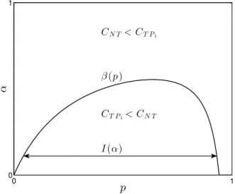
Next, we compareT P1andN T, and thereby provide a complete prescription for finding the best policy among the four policies. First defineα= h2/τ2
h1/τ1 to be a measure of the relative “importance” of
type-1 jobs over type-2 jobs. Note thatα∈(0,1)by Assumption 3.2.1. Ifαis close to 0, type-1 jobs are far more important than type-2 jobs; ifαis close to 1, there is no significant difference between the importance levels of the two types of jobs.
Proposition 3.3.2. For anyp∈(0,1),CT P1 ≤CN T if and only if0< α≤β(p), where
β(p) = max (
0, pτ1
N−2 N v1−2
u+pq(v1+v2−1)τ1τ2 qτ2
2− N−2
N (1−v2)
u+pq(v1+v2−1)τ1τ2
)
. (3.1)
In other words, Triage-Prioritize-Class-1 policy performs better than No-Triage policy, and thus is the
best policy among the four simple policies ifαis sufficiently small for a given value ofp; otherwise, No-Triage policy is the best policy.
Proposition 3.3.2 confirms the intuition that when the two types are sufficiently similar to each other - with regards to their importance - serving jobs randomly with no triage is superior to triaging them all (except for the last one). More specifically, the proposition gives a precise description of what we mean by two types of jobs beingsufficiently similar. The following corollary immediately follows from Propositions 3.3.1 and 3.3.2.
Corollary 3.3.1. Among the four policies,N T,T P1,T P2, andT AF, the best policy, i.e., the policy that minimizes the total expected cost, isT P1ifα≤β(p); otherwise, the best policy isN T.
in-sights into how the fraction of type-1 jobs in the population affects whether the differences between the two types of jobs would be significant enough to makeT P1 more preferable thanN T.
Proposition 3.3.3.β(·)is a quasi-concave function ofpand is first non-decreasing then non-increasing over(0,1). Thus, for each fixed0< α <1, there is an intervalI(α) = [p(α), p¯(α)], which is possi-bly an empty set and satisfies the following conditions:
(i) Ifp∈I(α),T P1is better thanN T; otherwise,N T is better.
(ii) 0< p(α) <p¯(α)<1, wherep(α)is a non-decreasing andp¯(α)is a non-increasing function ofα, i.e.,I(α)gets smaller asαincreases.
0 1
0 1
CN T< CT P1
CT P1< CN T β(p)
I(α)
p
α
Figure 3.1: Comparison of Triage-Prioritize-Class-1 (T P1) and No-Triage (N T) policies. (u = 0.15, v1 = 0.95, v2= 0.95, τ1= 1, τ2= 3, N = 100).
ends up being a waste of time, that is of course unless the two types are significantly different from each other as measured byα.
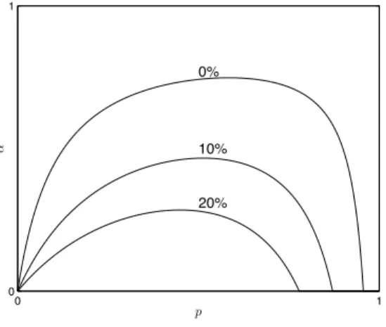
Propositions 3.3.3 shows that there is a unimodal curve that separates the Triage and No-Triage regions. We can strengthen this result further by showing that the benefit from triage (when there is) is smaller when one is close to the boundary described byβ(·)and gets large as one moves away. More precisely, define the percentage improvement by triage as
η≡ CN T −CT P1
CN T ×100%.
Proposition 3.3.4. For anyη >0, there exists a unimodal curveβ(p, η)such that
(i) CN T−CT P1
CN T > η0if and only ifα < β(p, η0)for any givenη0.
(ii) Ifη1 > η2, thenβ(p, η1)≤β(p, η2)for allp∈[0,1], and (iii) β(p, η) = max
(
0, pτ1
N−2
N v1−2
u+pq(v1+v2−1)τ1τ2−ηpτ1[N2−1τ1+pτ1+qτ2]
qτ2
2−NN−2(1−v2)u+pq(v1+v2−1)τ1τ2+ηqτ2[N2−1τ2+pτ1+qτ2] )
.
0 1
0 1
0%
10%
20%
p
α
Figure 3.2: Comparison of Triage-Prioritize-Class-1 (T P1) and No-Triage (N T) policies, different levels ofη.
is belowβ(p,10%), which implies that triage is more effective when there is significant difference between the two types of jobs, i.e.αis small.
3.3.2 Insights from comparison of policiesT P1andT P2
Our results provided a clear description of the conditions under whichN T andT P1 are the best policies among the four simple policies analyzed in this section. Clearly, there are many situations where skipping triage and serving jobs in random order is the best option. However, in many practical settings, because of unknown parameters such as p, it might be difficult to check whether or not the conditions are satisfied and as a result one might end up using a policy, which may or may not be optimal. Suppose for example that the service provider believes that all jobs should be triaged. (As many articles in the emergency response literature discuss, triage is performed in mass-casualty events despite the lack of any scientific evidence that it is actually beneficial.) The question then is whether priority should be given to class-1 jobs or class-2 jobs. More specifically, is it always true thatCT P1 ≤ CT P2? One might be tempted to believe that based on the classicalcµ-rule result, the
answer is yes and class-1 jobs should get a higher priority. After all, we know for a fact that if all jobs were already classified by time zero, the optimal action would have been to serve all class-1 jobs first. As we see in the following proposition, however, which only compares the policiesT P1 andT P2, this intuitive argument is flawed.
Proposition 3.3.5. (i) Ifv2<1/2−(NN pτ−2)u1 (v1+v2−1),thenCT P1 < CT P2 for allα∈(0,1);
(ii) ifv1<1/2−(NN qτ−2)u2 (v1+v2−1),thenCT P1 > CT P2 for allα∈(0,1);
(iii) otherwise,CT P1 < CT P2 if and only ifα < θ(p), where
θ(p) = min (
1, N−2
N pτ1(v1−1/2)u+pq(v1+v2−1)τ1τ2 N−2
N qτ2(v2−1/2)u+pq(v1+v2−1)τ1τ2
)
. (3.2)
Furthermore,θ(p)> β(p)forp∈(0,1).
small, thenT P2should be chosen over T P1. However, misclassification is not the only reason why T P2 can in fact be better thanT P1. Even if classification is perfect, i.e.,v1 =v2 = 1, as we can see from part (iii) of Proposition 3.3.5,T P2 is more preferable ifα > θ(p).
Before we explain why prioritizing less important jobs can in fact be better, first note the last statement of the proposition, which says thatθ(p)> β(p)forp∈(0,1). This fact together with the rest of the proposition and Proposition 3.3.2 implies thatT P2 can be better thanT P1 only ifN T is better than bothT P1 andT P2. In other words, doing triage and prioritizing class-2 can be better than prioritizing class-1 only when triage is in fact a waste of time and it is better to serve jobs in random order without triage anyway. But in any case, the result shows that if the service provider makes the mistake of doing triage somehow believing that itmust surelybe beneficial, s/he can make things even worse if s/he further prioritizes class-1 jobs based on a flawed intuitive argument.
3.3.3 Better triage better outcome?
Suppose that the service provider has the capability of improving triage accuracy possibly by more training, using an improved classification criteria, or using a more competent server. It is natural to expect that such an action should improve the outcome and in most cases it will. However, as we see in the following, this is not always true. The following proposition is an investigation into how the total expected cost underT P1 changes withv1 andv2, the probabilities of correct classification for types 1 and 2, respectively.
Proposition 3.3.6. (i) For all α ∈ (0,1) and p ∈ (0,1), ∂CT P1
∂v1 < 0, i.e., the expected cost
under the Triage-Prioritize-Class-1 Policy always decreases with the probability of correctly
classifying a type-1 job.
(ii) Let γ(p) = pτ1
pτ1+NN−2u
. For any fixedp ∈ (0,1), ifα > γ(p) then ∂CT P1/∂v2 > 0; i.e., if
α > γ(p), then the expected cost under the Triage-Prioritize-Class-1 Policy increases with the
probability of correctly classifying a type-2 job. Furthermore,γ(p)is an increasing function of pandβ(p)< γ(p)for anyp∈(0,1).
Part (i) of Proposition 3.3.6 is intuitive. It simply says that an improvement in triage, which results in a higher probability of correct classification for type-1 jobs, also improves the performance ofT P1. On the other hand, part (ii), which says that, in some cases an improvement in the correct classification probability of type-2 jobs worsens the performance of the policy, is not as intuitive. It is true thatT P1 does not aim to prioritize type-2 jobs, but regardless, a higher probability of correct classification means a better way of sorting out the two types. Given this fact, why should a higher value ofv2not always help?
of type-1 jobs is small. Thus, under policyT P1, significant time will be spent on identifying (possibly incorrectly) type-1 jobs, and a high percentage of jobs (all class-2 jobs) will have to wait the triage of all jobs to be over. It would actually be better if some of these jobs, if not all, were served before, right after they were triaged even if they belong to class-2. This is exactly what would happen if more of the type-2 jobs were misclassified as class-1 and therefore a decrease in correct classification probability for type-2 jobs helps.
3.4 State-dependent policies
In the previous section, we restricted ourselves to four policies, which are practically appealing because of their simplicity. In this section, we make no such restriction and concentrate on identifying the policy that is optimal within the whole class of state-dependent policies (which also includes state-independent policies). We first develop a Markov decision process (MDP) formulation for the problem described in Section 3.4.1 and then provide a complete description of the optimal policy.
3.4.1 Markov decision process formulation
The decision epochs are time zero, and triage and service completion times for the server (since we assume the service is non-preemptive). The state of the system can then be denoted by the triplet
(i, k1, k2), whereirepresents the number ofuntriagedjobs, andk1andk2denote the number of jobs that have been classified as class-1 and class-2 but not yet served, respectively. Since we haveN jobs in total, the state space can be described asS ={(i, k1, k2) :i, k1, k2≥0, i+k1+k2≤N}.
Using a sample-path argument, it is straightforward to show that keeping the server idle is subop-timal. This allows us to ignore idling as an admissible action. Then, in a given states = (i, k1, k2), the available actions for the server areSU: serve an untriaged job without triage (only available if i≥1);Tr: triage an untriaged job (only available ifi≥1);SC1:serve a class-1 job (only available ifk1 ≥1); andSC2:serve a class-2 job (only available ifk2≥1).
While this assumption is not crucial, it allows us to ensure that there is a unique optimal policy, which in turn simplifies the presentation of the results.
We definea∗(s)fors∈ Sto be the optimal action in states. We also letVπ(i, k1, k2)denote the total expected cost under policyπ andV(i, k1, k2) = minπ{Vπ(i, k1, k2)} to be the total expected cost under an optimal policy starting from state(i, k1, k2)with no service or triage in progress.
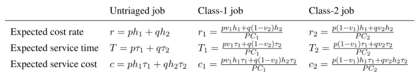
Table 3.1: Notation used in writing optimality equations in a compact form.
Untriaged job Class-1 job Class-2 job
Expected cost rate r =ph1+qh2 r1 = pv1h1+q(1−v2)h2
P C1 r2=
p(1−v1)h1+qv2h2
P C2
Expected service time T =pτ1+qτ2 T1 = pv1τ1+q(1−v2)τ2
P C1 T2 =
p(1−v1)τ1+qv2τ2
P C2
Expected service cost c=ph1τ1+qh2τ2 c1= pv1h1τ1+q(1P C1−v2)h2τ2 c2 = p(1−v1)hP C1τ12+qv2h2τ2
LetP Ci denote the probability of classifying a random job as class-ifori = 1,2so thatP C1 =pv1+
q(1−v2)andP C2 = p(1−v1) +qv2. Then, using the notation in Table 3.1 we can write the optimality
equations as follows:
V(i, k1, k2) = min
P C1V(i−1, k1+ 1, k2) +P C2V(i−1, k1, k2+ 1) + (ir+k1r1+k2r2)u
V(i−1, k1, k2) +c+ [(i−1)r+k1r1+k2r2]T,
V(i, k1−1, k2) +c1+ [ir+ (k1−1)r1+k2r2]T1,
V(i, k1, k2−1) +c2+ [ir+k1r1+ (k2−1)r2]T2
, ∀(i, k1, k2)∈S\(0,0,0),
V(0,0,0) = 0, andV(s) =∞, ∀s6∈S.
(3.3)
3.4.2 Complete characterization of the optimal policy
We start by describing when SC1 and SC2 are optimal actions.
Theorem 3.4.1. Consider state(i, k1, k2)∈ S:
(i) Ifk1 ≥1, thena∗(i, k1, k2) =SC1, i.e., as soon as the server identifies a class-1 job, that job should be served next.
Theorem 3.4.1 clearly delineates the regions where serving jobs classified as class-1 and class-2 are optimal. Specifically, SC1 has precedence over all other actions no matter what the current state is. This means that as soon as a triage results in identification of a class-1 job, the next action is to serve that job. On the other hand, SC2 is at the bottom of the priority list meaning that the service of class-2 jobs starts at the end when there are no more class-1 or untriaged jobs waiting.
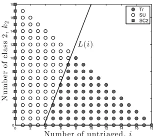
Given Theorem 3.4.1, to characterize the optimal policy completely, it now remains to study the states where there are no class-1 jobs, i.e.,k1 = 0, but there is at least one untriaged job, i.e.,i≥1. Recall that in such a state, the server can choose to either triage or directly serve an untriaged job. We know that serving a class-2 job, if there is one, is suboptimal. It turns out that whether or not doing triage is optimal depends on the system state. More specifically, there is a line that separates the states in which doing triage is optimal from the states in which serving without triage is optimal. With the following theorem, we not only prove this structural property of the optimal policy but also provide a complete expression for this line.
Theorem 3.4.2. There exists a linear functionL(·)such that for any state(i,0, k2)∈ Swherei≥1 andk2 ≥ 0, ifk2 ≥L(i), thena∗(i,0, k2) =SU, i.e., the optimal action is to serve without triage; otherwise,a∗(i,0, k
2) =Tr, i.e., the optimal action is to perform triage. Furthermore,
L(i) =
r(˜u−u)
r2u
i− ru˜
r2u, (3.4)
whereu˜=P C2(rT2−r2T)/r.
0 2 4 6 8 10 12 14 16 18 0
2 4 6 8 10 12 14 16 18
Numb er of untriaged, i
N
u
m
b
er
o
f
cl
a
ss
2
,
k2
L(i)
Tr SU SC2
Figure 3.3: Visual description of the optimal policy whenk1 = 0andh1 = 10, h2 = 1, τ1 = 1, τ2 = 2, v1 = 1, v2= 0.95, u= 0.26, p= 0.8, N = 18.
Theorem 3.4.2 provides interesting insights into the decision of when to do triage and when to skip it. IfN is large, meaning that there are too many jobs waiting to be served and we have no information regarding which ones are more important, one might be tempted to skip triage since performing triage will further lengthen the waiting times, which are already likely to be too long. With too many jobs to serve, spending time on triage might seem like an unwise use of time. In contrast, whenN is small, triage might not seem all that harmful since waiting times are not going to be too long even with triage. As we explain in the following, however, this reasoning is flawed.
to spend some time at the beginning (specifically as long as the system state is to the right of the threshold line) to perform triage in an effort to at least prevent the waiting times for important jobs getting too long. On the other hand, when there are few jobs, service of all jobs including those of type-1, will not take too much time. Therefore, the value of class information that will be obtained through triage does not justify the additional waiting that all jobs will have to endure.
Finally, in this section, we investigate conditions under which the optimal policy turns out to be one of the simple benchmark policies investigated in Section 3.3. It would be natural to expect that under the optimal policy, when the expected triage time is sufficiently short (it might help to think of the limiting case where it is zero) all jobs would go through triage and when the expected triage time is sufficiently long no job would go through triage. Indeed, we can prove that is the case. The following proposition clearly describes what would qualify as sufficiently short and what would qualify as sufficiently long.
Proposition 3.4.1. Letu1 = NN−1u˜andu2= 2r+(Nr−2)r
2u˜. Then,
(i) the optimal policy isN T, i.e., No-Triage policy, if and only ifu≥u1;
(ii) the optimal policy isT P1, i.e., Triage-Prioritize-Class-1 policy, if and only ifu≤u2.
When the expected triage time is as long as described in Proposition 3.4.1(i), the information that one would get through triage is simply not worth it. Hence, the optimal policy is to serve all jobs directly without triage. When the expected triage time is as short as described in Proposition 3.4.1(ii), one can “afford” to triage all the jobs no matter what types of jobs are identified during the triage process; however, in line with Theorem 3.4.1, if a class-1 job is identified as a result of triage, that job should be served first before moving on to the triage of the remaining jobs.
3.5 Numerical study: performance comparison of the proposed policies under linear and non-linear waiting costs
waiting costs are linear functions of time as are assumed in our mathematical model. In the second part, based on our analytical results given in Section 3.4, we first devise heuristic methods that can be used when waiting costs are not linear. Then, we compare the performances of these heuristic methods with those of the optimal policy as well as the simple benchmark policies.
3.5.1 Performance comparison when waiting costs are linear in time
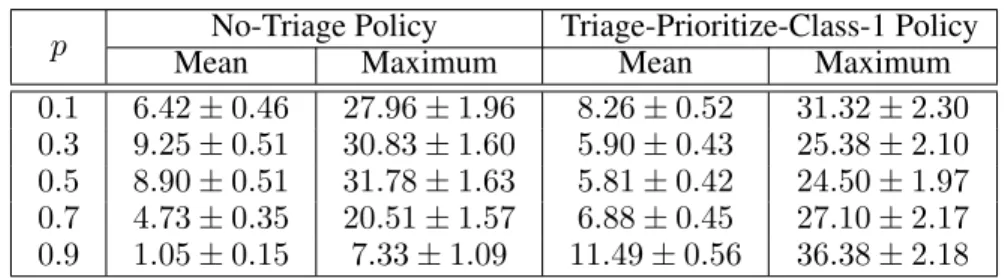
For this study, we considered a system withN = 50jobs, all untriaged at time zero. We chose p from the set {0.1,0.3,0.5,0.7,0.9}, and for each value of p, we generated 2,000 scenarios by randomly and uniformly choosingubetween 0 and 1,τ1andτ2 between 0 and 10,h1between 0 and 4, h2 between 0 and 1, v1 andv2 between 0.5 and 1; discarding cases for which h1/τ1 < h2/τ2. For each scenario, we obtained the total expected cost under the optimal policy, No-Triage policy (N T), and Triage-Prioritize-Class-1 policy (T P1), and computed the percentage improvement in the total expected cost that one would get by using the optimal policy as opposed to each one of the benchmark policies N T and T P1. Then, we constructed 95% confidence intervals for the mean percentage improvement as well as the maximum percentage improvement. (The confidence interval for the maximum percentage improvement was obtained by putting the 2,000 scenarios in groups of size 10 and determining the maximum within each group, which results in a total of 200 observations.) The results are provided in Table 3.2.
Table 3.2: 95% confidence intervals for the mean and maximum percentage improvement in the total expected cost by using the optimal policy as opposed to benchmark policies.
p No-Triage Policy Triage-Prioritize-Class-1 Policy
Mean Maximum Mean Maximum
0.1 6.42±0.46 27.96±1.96 8.26±0.52 31.32±2.30 0.3 9.25±0.51 30.83±1.60 5.90±0.43 25.38±2.10 0.5 8.90±0.51 31.78±1.63 5.81±0.42 24.50±1.97 0.7 4.73±0.35 20.51±1.57 6.88±0.45 27.10±2.17 0.9 1.05±0.15 7.33±1.09 11.49±0.56 36.38±2.18
zero or 1,N T is the best benchmark policy for a large range of values ofα(it performs particularly well whenpis close to 1) and thus it is no surprise that its performance is closer to that of the optimal policy for such values ofp. The performance gap is more significant for mid-range values ofp. When comparing the performances of the optimal policy andT P1, we observe the opposite. T P1performs relatively better for mid-range values ofp. This is not surprising. N T andT P1 can be seen as at the two ends of the policy spectrum with the former skipping triage altogether and the latter performing triage for all the jobs. Thus when jobs are highly dominated by one type,N T tends to perform better since triage does not bring much benefit; when there is a good mixture of both types,T P1 tends to perform better. The optimal dynamic policy hits the “right” balance between these two policies by choosing to triage or skip it depending on the system state.
3.5.2 Performance comparison when waiting costs are non-linear in time
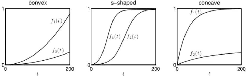
One of the assumptions we made for our mathematical analysis was that the cost of keeping the jobs waiting is linear in time. There are, however, situations where this assumption would not be reasonable. Our goal in this section is to propose new heuristic methods based on our analysis under the linear waiting cost assumption and test how these methods perform in comparison with other benchmark heuristics when waiting costs are non-linear in time. In particular, we consider three different forms for the waiting cost function: increasing convex, increasing concave, and increasing convex-concave (S-shaped). In the following, we will usef1(·)andf2(·)to denote the waiting cost functions for types 1 and 2, respectively, i.e.,fi(t)is the total cost that would be incurred by a type-i job that has waited forttime units in the system.
Proposed heuristic methods to be used when waiting costs are non-linear
We propose three heuristic methods:
expected time the system would be cleared of all jobs if each job were to go through triage. We name the heuristic Fixed Threshold-cµpolicy because (i) whether or not triage is carried out in a given state is determined by where the state lies with respect to the threshold line, which is fixed at time zero, and (ii) class-1 (high priority) and class-2 (low priority) are determined according to the expected version of thecµ-rule. Note that thecterm here is calculated using the slopes of the fitted lines for each type.
(ii) Dynamic Threshold-cµpolicy (DT-cµ):We fit a least-squares line to each cost function and, as in theF T-cµpolicy, use the slopes of these lines to determine the high priority class and the low priority class with respect to thecµ-rule. Unlike theF T-cµpolicy, however, this policy updates the threshold line to be used for determining whether or not triage should be done by fitting new least-squares lines over the interval[tnow, tnow+i(τ+u)+k1τ1+k2τ2]wheretnow is the current time, i.e., the time decision is to be made, andtnow+i(τ +u) +k1τ1+k2τ2 is the expected time the system would be cleared of all jobs if each remaining untriaged job were to go through triage. The time-dependent threshold lineLt(·)is obtained by using (3.4) but replacingh1andh2with the slopes of the two lines fitted tof1(·)andf2(·), respectively. (iii) Dynamic Threshold-Gcµpolicy (DT-Gcµ):This policy updates the threshold line exactly the
Numerical experiments and results
In our numerical study, we mainly considered three different scenarios each differing in the general structure for the waiting cost functions assumed. For each pair of cost function choices, we generated scenarios as follows: we assumed that initally there were 20 jobs all untriaged. The expected triage time was assumed to be 0.5 units. The expected service timeτ was assumed to be the same for both types and was chosen from the set{1,5,10}. The probability of a random job being of type 1,p, was chosen from the set{0.1,0.3,0.5,0.7,0.9}. For each pair of τ andp values chosen, 200 scenarios were randomly generated by choosing bothv1 andv2uniformly between 0.5 and 1. Triage times and service times were assumed to be deterministic so as to make it possible to obtain the optimal policy and compare its performance with those of the heuristic methods.
Convex increasing waiting cost functions:As discussed in detail in Van Mieghem (1995), for vari-ous reasons including customer expectations and the psychology of waiting, in certain settings a con-vex function that penalizes waits with an increasing rate might be a better fit. To investigate how the proposed methods might work in such settings, we assumed thatf1(t) = 210t 2andf2(t) = 14 210t 2
(see the leftmost plot in Figure 3.4).
0 200
0 1
convex
f1(t)
f2(t)
t 0 200
0 1
s−shaped
f1(t) f2(t)
t 0 200
0 1
concave f1(t)
f2(t)
t
Figure 3.4: The waiting cost functions assumed in the numerical study.
in that parameter region. However, No-Triage policy performs poorly when the expected service time is significantly larger than the expected triage time. We also observe that the benchmark policiesT P1 andT P2perform badly across almost all scenarios.
Table 3.3: Performance comparison for the convex cost case - 95% confidence interval for the mean percentage increase in total expected cost when compared with that under the optimal policy.
τ p F T-cµ DT-cµ DT-Gcµ N T T P1 T P2
1 0.1 0.00±0.00 0.00±0.00 0.00±0.00 0.00±0.00 163.58±1.59 198.47±1.80 1 0.3 0.00±0.00 0.00±0.00 0.00±0.00 0.00±0.00 133.82±2.85 229.68±2.94 1 0.5 0.00±0.00 0.00±0.00 0.00±0.00 0.00±0.00 128.28±3.20 231.57±2.92 1 0.7 0.00±0.00 0.00±0.00 0.00±0.00 0.00±0.00 133.95±3.04 222.21±2.41 1 0.9 0.00±0.00 0.00±0.00 0.00±0.00 0.00±0.00 146.26±2.57 207.96±1.76 5 0.1 0.12±0.03 0.12±0.03 0.12±0.03 0.65±0.16 15.01±0.60 46.91±1.17 5 0.3 0.26±0.03 0.26±0.03 0.26±0.03 6.20±0.89 8.06±0.66 68.00±3.03 5 0.5 0.14±0.02 0.14±0.02 0.14±0.02 5.48±0.88 7.38±0.74 63.39±2.72 5 0.7 0.03±0.01 0.03±0.01 0.03±0.01 1.31±0.34 9.80±0.89 48.04±1.29 5 0.9 0.00±0.00 0.00±0.00 0.00±0.00 0.00±0.00 18.76±0.61 35.86±0.35 10 0.1 0.29±0.03 0.29±0.03 0.29±0.03 4.20±0.48 4.37±0.25 36.41±1.58 10 0.3 0.19±0.02 0.19±0.02 0.19±0.02 14.64±1.40 2.15±0.19 62.14±3.57 10 0.5 0.11±0.01 0.11±0.01 0.11±0.01 13.83±1.42 1.86±0.21 56.86±3.27 10 0.7 0.07±0.01 0.07±0.01 0.07±0.01 6.68±0.84 2.34±0.31 37.98±1.84 10 0.9 0.00±0.00 0.00±0.00 0.00±0.00 0.06±0.04 6.19±0.44 19.64±0.28
S-shaped (convex-concave) increasing waiting cost functions:In the case of emergency response or search and rescue operations, jobs may correspond to injured individuals whose survivals are at stake. With passage of time, the survival probabilities of these individuals decline. In many cases, the way these survival probabilities decline with time has an inverse S-shape with the survival probabilities declining with a rate that is slow at the beginning but gradually getting faster but eventually getting slow again when the survival probabilities get closer to zero (Sacco et al., 2005). This corresponds to a waiting cost function, which has an S-shape with a convex increasing portion at the beginning followed by a concave increasing portion. To investigate how the proposed methods work when waiting cost functions have such a structure, we assumed thatf1(t) = 1+e−61t/75+4−
1
1+e4 andf2(t) =
1
1+e−4t/75+5.5 −
1
1+e5.5. These two functions are plotted in the middle graph in Figure 3.4. Bothf1(·)
that the rate of increase in the waiting cost is not always higher for type-1 jobs. Their costs increase with a rate that is higher than that for type-2 jobs initially but once their cost gets sufficiently close to 1, the rate for type-2 jobs gets higher.
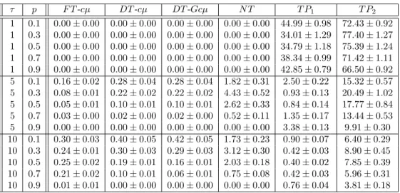
Table 3.4: Performance comparison for the S-shaped cost case - 95% confidence interval for the mean percent-age increase in total expected cost when compared with that under the optimal policy.
τ p F T-cµ DT-cµ DT-Gcµ N T T P1 T P2
1 0.1 0.00±0.00 0.00±0.00 0.00±0.00 0.00±0.00 100.99±2.21 183.80±2.68 1 0.3 0.00±0.00 0.00±0.00 0.00±0.00 0.00±0.00 85.97±3.38 213.33±3.61 1 0.5 0.00±0.00 0.00±0.00 0.00±0.00 0.00±0.00 91.53±3.40 207.98±3.08 1 0.7 0.00±0.00 0.00±0.00 0.00±0.00 0.00±0.00 104.40±2.98 194.10±2.28 1 0.9 0.00±0.00 0.00±0.00 0.00±0.00 0.00±0.00 121.57±2.30 177.74±1.52 5 0.1 0.00±0.00 0.00±0.00 0.00±0.00 0.00±0.00 24.13±0.57 36.46±0.53 5 0.3 1.23±0.19 1.22±0.20 1.09±0.19 2.15±0.43 11.11±0.54 38.09±1.21 5 0.5 1.71±0.26 1.70±0.27 1.22±0.19 2.36±0.43 9.31±0.36 36.45±1.41 5 0.7 0.65±0.17 0.57±0.14 0.36±0.09 0.58±0.15 9.51±0.27 29.32±0.90 5 0.9 0.01±0.00 0.00±0.00 0.00±0.00 0.01±0.00 10.93±0.18 21.35±0.38 10 0.1 0.11±0.03 0.01±0.00 0.04±0.01 0.11±0.03 9.19±0.10 3.60±0.18 10 0.3 2.99±0.27 0.71±0.08 1.30±0.13 2.99±0.27 13.48±0.51 3.05±0.16 10 0.5 4.72±0.38 2.04±0.25 2.02±0.18 4.72±0.38 15.62±0.72 4.51±0.30 10 0.7 4.05±0.31 2.72±0.35 1.53±0.14 4.05±0.31 12.66±0.56 6.12±0.45 10 0.9 1.33±0.10 0.95±0.12 0.26±0.02 1.33±0.10 5.79±0.16 5.72±0.32
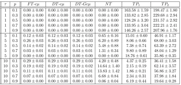
The results are given in Table 3.4. When the expected service time is short meaning that triage times are relatively long, No-Triage policy turns out to be optimal along with all three policies we are proposing. As the expected service time gets longer, we start seeing some differences among the four policies. First of all, No-Triage policy is no longer optimal even though its performance is still very reasonable and very close to that of theF T-cµpolicy. In fact, theF T-cµpolicy simplifies to the No-Triage policy in most cases. In some cases, F T-cµ outperforms the No-Triage policy but nevertheless it is still difficult to make a strong argument thatF T-cµwould be a better choice than No-Triage considering the simplicity of the latter policy. However, the performances of bothDT-cµ andDT-Gcµare superior to those of F T-cµand the No-Triage policy in all the settings where the expected service time is large relative to the expected triage time and very close to that of the optimal policy in all the settings. In particular, the worst performance ofDT-Gcµis observed whenp = 0.5
Concave increasing waiting cost functions: In some cases, concave functions can more appro-priately capture the reality. For example, consider an emergency response situation which leads to S-shaped waiting cost functions as discussed above. Now, suppose that due to the delays in response, which might have various reasons, the service process starts long after the incident occurred and as a result we are faced with only the concave increasing portion of the waiting cost function. To inves-tigate how our policies would perform in such settings, we assumed thatf1(t) = 1−e(−0.03)t and f2(t) = (1−e(−0.01)t)/4, which are both concave increasing functions (see the rightmost graph in Figure 3.4 for plots of these two functions).
Table 3.5: Performance comparison for the concave cost case - 95% confidence interval for the mean percentage increase in total expected cost when compared with that under the optimal policy.
τ p F T-cµ DT-cµ DT-Gcµ N T T P1 T P2
1 0.1 0.00±0.00 0.00±0.00 0.00±0.00 0.00±0.00 44.99±0.98 72.43±0.92 1 0.3 0.00±0.00 0.00±0.00 0.00±0.00 0.00±0.00 34.01±1.29 77.40±1.27 1 0.5 0.00±0.00 0.00±0.00 0.00±0.00 0.00±0.00 34.79±1.18 75.39±1.24 1 0.7 0.00±0.00 0.00±0.00 0.00±0.00 0.00±0.00 38.34±0.99 71.42±1.11 1 0.9 0.00±0.00 0.00±0.00 0.00±0.00 0.00±0.00 42.85±0.79 66.50±0.92 5 0.1 0.16±0.02 0.28±0.04 0.28±0.04 1.82±0.31 2.50±0.22 15.32±0.57 5 0.3 0.08±0.01 0.22±0.02 0.22±0.02 4.43±0.52 0.93±0.13 20.49±1.02 5 0.5 0.05±0.01 0.10±0.01 0.10±0.01 2.62±0.33 0.84±0.14 17.77±0.84 5 0.7 0.03±0.00 0.02±0.00 0.02±0.00 0.52±0.11 1.35±0.17 13.44±0.53 5 0.9 0.00±0.00 0.00±0.00 0.00±0.00 0.00±0.00 3.38±0.13 9.91±0.30 10 0.1 0.30±0.03 0.40±0.05 0.42±0.05 1.73±0.23 0.90±0.07 6.40±0.29 10 0.3 0.24±0.01 0.30±0.03 0.29±0.03 3.12±0.30 0.42±0.03 8.90±0.45 10 0.5 0.25±0.02 0.19±0.01 0.16±0.01 2.03±0.18 0.40±0.02 7.85±0.39 10 0.7 0.21±0.02 0.10±0.01 0.06±0.01 0.75±0.08 0.42±0.03 5.96±0.31 10 0.9 0.01±0.01 0.00±0.00 0.00±0.00 0.00±0.00 0.76±0.04 3.81±0.18
CHAPTER 4: PRIORITY SCHEDULING OF JOBS WITH HIDDEN TYPES IN A QUEUEING SYSTEM
4.1 Introduction
In this chapter, we study the information/delay trade-off in a setting where there are external arrivals to the system. Jobs, which arrive at the system, are of unknown type, and similar to the model in Chapter 3, the server has the option to spend time to extract the type information for each job. The queueing model in this chapter incorporates the feature that in an MCI, injuries may arrive or be transported to the triage/treatment field. Our objective is to study the optimal dynamic policy on whether to triage or skip triage in order to minimize the long-run average cost.
The remainder of this chapter is organized as follows: Section 4.2 gives a detailed description of the formulation. Section 4.3 shows that there exists a threshold type policy that is optimal, and describes how we prove this results. A simulation study is carried out in Section 4.4. We observe that a heuristic policy we propose, which mimics the properties of the optimal policy, can bring significant improvement over simple and easy-to-implement policies.
4.2 Model description
We assume that the type information of each new job is hidden from the service system initially, i.e., the server does not know the exact type of a new arrival. The server can serve a job without knowing its type, but s/he also has the option to spend some time on investigation to obtain the type information of a job, and classify the job as class 1 or class 2. The investigation time of a job is exponentially distributed with meanu >0,independent of the arrival process and the job’s type. We denote class 1 as the important class, and class 2 as the less important class. The server tries her/his best to classify the type 1 jobs into class 1, and type 2 jobs into class 2. While the investigation on a job provides information on the job’s type, the classification is error-prone. Definev1 as the probability of classifying a type 1 job into class 1 andv2as the probability of classifying a type 2 job into class 2. Without loss of generality, we assume thatv1+v2 >1.DenoteP Cias the probability of classifying a random job into classi, wherei= 1,2. Then,P C1 =pv1+q(1−v2), P C2 =p(1−v1) +qv2.
We further assume that a preemptive discipline is used and there is no cost or changeover time for the server to switch actions. Let xj(t) denote the number of jobs in class j at time t where j= 0,1,2,thenX(t) = (x0(t), x1(t), x2(t))is the current state of the system. Hence, the state space isS = {(i, k1, k2) : i ≥ 0, k1 ≥ 0, k1 ≥ 0}.At any time, the provider of the service system can take one of the following four actions: SU– serve an untriaged job without triage (only available if i≥1);Tr– triage an untriaged job (only available ifi≥1);SC1– serve a class-1 job (only available ifk1 ≥1); andSC2– serve a class-2 job (only available ifk2≥1).
One can easily show that unforced idling is suboptimal due to the preemption assumption. Denote the action set byA= {SC1, SU, T r, SC2}and the action taken at timetbya(t).A control policy π specifies the action taken at timetgiven the current system state X(t).Hence, we only consider control policies with Markovian properties. Our objective is to minimize the expected average cost per unit time over an infinite horizon which is formally defined as
g(π, s) = lim sup
n→∞
Vn(π, s)
n , ∀s∈ S,
over all the other actions. While this assumption is not crucial, it allows us to ensure that there is a unique optimal policy, which in turn simplifies the presentation of the results. Denote the optimal action atX(t)bya∗(X(t))and optimal expected average cost byg∗(s) :
g∗(s) = inf
π∈Πg(π, s), ∀s∈ S, (4.1)
4.3 State-dependent policies
4.3.1 Markov decision process formulation
Letrbe the expected cost rate for an untriaged job, andri be the expected cost rate for a class-i job,i= 1,2,then
r =ph1+qh2, r1 =
pv1h1+q(1−v2)h2 P C1
, r2 =
p(1−v1)h1+qv2h2 P C2
. (4.2)
Throughout the rest of this chapter, we assume thatuniformizationhas been applied with the following uniformization constant
φ=λ+1
u +
1
τ.
Without loss of generality we assumeφ= 1.Thus, instead of considering the above continuous-time problem, we study the discrete-time equivalent. Letting for(i, k1, k2) ∈ S, v/ (i, k1, k2) = ∞,the optimality equations can be written as follows. For(i, k1, k2)∈ Sandi+k1+k2>0,
v(i, k1, k2) +g=λv(i+ 1, k1, k2) +ir+k1r1+k2r2+ min
n
1
u
P C1v(i−1, k1+ 1, k2) +P C2v(i−1, k1, k2+ 1)+ 1
τv(i, k1, k2),
1
τv(i−1, k1, k2) +
1
uv(i, k1, k2),
1
τv(i, k1−1, k2) +
1
uv(i, k1, k2),
1
τv(i, k1, k2−1) +
1
uv(i, k1, k2)
o
,
v(0,0,0) +g=λv(1,0,0) + 1
τv(0,0,0) +
1
uv(0,0,0).
(4.3)
above optimality equations. Moreover, there exists a stationary policy that is optimal for the above
problem.
4.3.2 Characterization of the optimal policy
The following theorem presents our main theoretical result, which describes the structure of the optimal policy as of threshold type.
Theorem 4.3.1. There exists an optimal policy that can be described as follows:
(i) Ifk1 ≥ 1, thena∗(i, k1, k2) = SC1, i.e., once the server identifies a class-1 job, the server should serve this job immediately.
(ii) The optimal actiona∗(i, k1, k2) =SC2only wheni= 0andk2 = 0, i.e., the server serves a class-2 job only when there are no class-0 or class-1 jobs in the system.
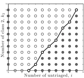
(iii) Ifk1 = 0andi >0, then for eachi≥1,there exists a thresholdk2∗(i)such that ifk2 < k∗2(i), the optimal action is triage; otherwise, serve without triage.
(iv) Ifu≥u˜:=P C2(r−r2)τ /r, thena∗(i,0, k2) =SU for all(i,0, k2)∈S.
This theorem establishes that for any given time and specified number of jobs of a given class (e.g., class-0, class-1, class-2), it is optimal to give class-1 jobs the highest priority and class-2 jobs the lowest priority. If there are no class-1 jobs, the server should triage a class-0 job if the number of the class-2 jobs is below a critical value, and serve a class-0 job directly without triage when the number of class-2 jobs is sufficiently large. The results agree with the well-knowncµrule, which gives priority to class-1 jobs over class-0 jobs and gives priority to class-0 jobs over class-2 jobs if triage is not an option. When there are many class-2 jobs (less-importance jobs) waiting for service, the value of job type information that will be obtained through triage could not compensate the additional delay that the remaining jobs will have to suffer. Hence, the optimal action is to skip triage. When triage takes a significant amount of time, the threshold,k∗
0 1 2 3 4 5 6 7 8 9 10 11 0
1 2 3 4 5 6 7 8 9 10 11
Numb er of untriaged, i
N
u
m
b
e
r
o
f
c
la
ss
2
,
k2
Figure 4.1: Visual description of the optimal policy whenk1 = 0andλ= 0.6, h1 = 10, h2 = 1, τ1 =τ2 = 1, v1= 0.9, v2= 0.95, u= 0.25, p= 0.6.
An example of the threshold-type policy, determined by solving the Bellman’s equation in (4.3) recursively, is presented in Figure 4.1. Thex-axis represents the number of class-0/untriaged jobs and they-axis represents the number of class-2 jobs in the system. The threshold-type policy, described in Theorem 4.3.1, reflects the real-time decision on whether to triage or not.
The proof follows after showing some properties of the optimal value functionsv(i, k1, k2).We first show that the desired properties for the value functions of the discounted version of the model are preserved under the value-iteration operator with small discount factor, then we show that such properties hold when the discount factor is approaching0,which implies that the optimal value func-tions in the case of long-run average cost preserve such properties as well. The technical details are presented in Section 4.3.3.
Proposition 4.3.2. If
λ≤ τ−u τ2
1− τ τ−u
r2
(˜u/u−1)r+r2
,
thenk∗2(i)increases withi.