Exploring Star Formation In Cluster Galaxies

(1)

University of North Dakota

UND Scholarly Commons

Theses and Dissertations Theses, Dissertations, and Senior Projects

January 2018

Exploring Star Formation In Cluster Galaxies

Sandanuwan Prasadh Kalawila Vithanage

Follow this and additional works at:https://commons.und.edu/theses

Recommended Citation

Kalawila Vithanage, Sandanuwan Prasadh, "Exploring Star Formation In Cluster Galaxies" (2018).Theses and Dissertations. 2247.

(2)

EXPLORING STAR FORMATION IN CLUSTER

GALAXIES

by

Sandanuwan Kalawila Vithanage

Bachelor of Science, University of Ruhuna, Matara, Sri Lanka, 2009

A Dissertation

Submitted to the Graduate Faculty of the

University of North Dakota in partial fulfillment of the requirements

for the degree of Doctor in Philosophy

Grand Forks, North Dakota August

(3)

(4)

(5)

Permission

Title Exploring Star Formation in Cluster Galaxies

Department Physics and Astrophysics Degree Doctor of Philosophy

In presenting this dissertation in partial fulfillment of the requirements for a graduate degree from the University of North Dakota, I agree that the library of this University shall make it freely available for inspection. I further agree that permission for extensive copying for scholarly purposes may be granted by the professor who supervised my dissertation work or, in his absence, by the chairperson of the department or the dean of the Graduate School. It is understood that any copying or publication or other use of this dissertation or part thereof for financial gain shall not be allowed without my written permission. It is also understood that due recognition shall be given to me and to the University of North Dakota in any scholarly use which may be made of any material in my dissertation.

Sandanuwan Kalawila Vithanage 07/11/2018

(6)

LIST OF FIGURES

1.1 Tuning fork diagram for rich clusters (Rood and Sastry 1971). . . 3

1.2 Galaxies of di↵erent morphologies. . . 5

1.3 Galaxy morphologies as a function of clustercentric radius. . . 6

1.4 Hubble’s tuning fork diagram. . . 7

1.5 Relation between non-thermal radio and the far-infrared emission. . . 11

1.6 Emission ofH↵ photons. . . 11

1.7 Star formation density as a function of redshift . . . 14

1.8 Schematic diagram of dynamical friction. . . 16

1.9 Ram pressure stripping of a spherically symmetric gas distribution. . 19

1.10 Ram pressure stripping of ESO 137-001 galaxy in Abell 3627 cluster. 20 1.11 NGC 4402: falling towards the Virgo Cluster . . . 21

2.1 KPNO 4-m telescope. . . 24

2.2 CCD orientation of Mosaic-1.1. . . 25

2.3 CCD orientation of Mosaic-3. . . 26

2.4 Filter transmission curve for the r-band filter. . . 27

2.5 Filter transmission curve for the K1059 filter. . . 28

2.6 Filter transmission curve for the K1060 filter. . . 28

2.7 Narrow-band filter transmission curves compared to the broad band filter. . . 29

2.8 Spatial distribution of observed galaxy clusters. . . 31

3.1 CCD water bucket analogy . . . 34

3.2 A426 cross talk correction. . . 37

3.3 Pupil images. . . 38

3.4 Flat field correction of A426 r. . . 39

3.5 Median-filtered sky flat field image. . . 40

3.6 A2107 raw image . . . 41

3.7 Calibrated A2107 cluster image. . . 42

3.8 A757 WCS o↵set. . . 46

3.9 A757 spatial distribution of fitting . . . 46

3.10 Residuals of x WCS fitting . . . 47

(12)

3.17 Narrow-band image of Abell 496. . . 56

3.18 r-band image of Abell 576. . . 57

4.1 Schematic diagram of image subtraction. . . 74

4.2 PSF of a star. . . 75

4.3 Seeing comparison. . . 76

4.4 A426 flux ratio . . . 77

4.5 Image subtraction. . . 78

4.6 A426 object detection using PPP. . . 79

4.7 PPP classification: C2 vs instrumental magnitudes. . . 84

4.8 A1983 PPP variable classification. . . 85

4.9 IRAF ELLIPSE modeling . . . 87

4.10 A426 BCG model. . . 88

5.1 A2107 zero point calibration. . . 91

5.2 Completeness limit of A426. . . 93

5.3 Illustration of projection e↵ect of cluster galaxies. . . 94

5.4 Cluster red-sequence for Abell 426. . . 96

5.5 The rectified red-sequence for Abell 426. . . 96

5.6 Color histogram of red-sequence galaxies in Abell 426. . . 97

(13)

6.1 g-r red-sequence. . . 114

6.2 Log SFR vs (r/r200) . . . 116

6.3 Log EW and SFR. . . 117

6.4 Log EW vs (r/r200). . . 118

6.5 SSFR vs (r/r200). . . 120

6.6 Division into giant and dwarf galaxies. . . 121

6.7 DwarfMr vs (r/r200). . . 122

6.8 Log SFR vs (r/r200) for giants. . . 123

6.9 Log SFR vs (r/r200) for dwarfs. . . 123

6.10 Log EW vs (r/r200) for giants. . . 125

6.11 Log EW vs (r/r200) for dwarfs. . . 126

6.12 SSFR vs (r/r200) for giants. . . 127

6.13 SSFR vs (r/r200) for dwarfs. . . 128

6.14 Log SFR vs (r/r200) for giant ellipticals. . . 129

6.15 Log SFR vs (r/r200) for giant spirals. . . 129

6.16 Log EW vs (r/r200) for giant ellipticals. . . 131

6.17 Log EW vs (r/r200) for giant spirals. . . 132

6.18 SSFR vs (r/r200) for giant ellipticals. . . 133

6.19 SSFR vs (r/r200) for giant spirals. . . 134

6.20 Morphology-Density relation. . . 136

6.21 Red-sequence spirals. . . 137

6.22 WISE objects. . . 138

7.1 SFR and EW from Gomez et al. (2003). . . 140

7.2 SFR from Balogh et al. (2000). . . 142

7.3 SSFR from Von Der Linden et al. (2010). . . 147

7.4 Log SSFR vs (r/r200) for giant galaxies. . . 148

7.5 Log SSFR vs (r/r200) for dwarf galaxies. . . 148

7.6 Surface brightness profile of normal elliptical and cD galaxy. . . 149

(14)

LIST OF TABLES

2.1 Properties of Mosaic 1.1. . . 25

2.2 Properties of Mosaic-3. . . 26

2.3 Observed galaxy cluster sample. . . 31

3.1 Five-point dither pattern. . . 50

5.1 The r-band zero points for observed clusters. . . 91

5.2 Completeness limit of the cluster sample. . . 93

5.3 K-correction coefficients. . . 106

(15)

Acknowledgements

I would like to express my deepest gratitude to my advisor, Dr. Wayne Barkhouse, for providing me guidance, being there to discuss my research, and providing all the opportunities to explore the world of galaxies. I thank my graduate committee members: Dr. Timothy Young, Dr. Kanishka Marasinghe, Dr. Yen Lee Loh and Dr. Travis Desell for their comments and suggestions.

My sincere thanks to the Kitt Peak National Observatory for providing me observ-ing time and financial support. I would also like to thank the North Dakota NASA Established Program to Stimulate Competitive Research (EPSCoR) for providing financial support for my research.

My thanks to Cody Rude, Madina Sultanova, Haylee Archer, and Gregory Foote for helping me with observations at the KPNO 4-m telescope.

(16)

Dedications

To my parents, Chandrani and Chandrasoma,

(17)

ABSTRACT

Galaxy clusters are the most dense virialized environments in the known Universe. Hence they are the best locations to study the e↵ect of the high-density environment on the evolution of galaxies. The intracluster medium (ICM) plays an important role in galaxy evolution. The goal of this dissertation is to study the e↵ect of the ICM on galaxy evolution using star formation. A sample of 10 galaxy clusters were observed through the r-band and redshifted H↵ narrow-band filters using the Mayall 4-m telescope at the Kitt Peak National Observatory. Continuum image subtraction was used to measure H↵ flux to quantify star formation. Cluster galaxies were selected using the red-sequence method. The radial dependence (0.0  (r/r200)  1.0) of the star formation rate (SFR), equivalent width (EW), and specific star formation rate (SSFR) were measured for the cluster galaxy sample. Evidence for quenching of star formation towards the cluster center was found at all radii using the SFR, EW, and SSFR to estimate star formation activity. Results suggest that both galaxy harassment and ram pressure stripping help to quench star formation in the low-density cluster outskirts, while ram pressure stripping plays a more important role towards the high-density cluster center. The cluster galaxy sample was divided into giant (high-mass) and dwarf (low-mass) galaxies. It was found that dwarfs are more susceptible to ram pressure stripping than the giant systems. The e↵ect of the cluster environment on di↵erent morphological types, such as elliptical and spiral galaxies, was studied and it was determined that ram pressure and galaxy harassment have similar e↵ects on the SFR for both morphological types.

(18)

Chapter I

INTRODUCTION

1.1 Galaxy Clusters

Galaxies are not uniformly distributed throughout space. Instead, they have a ten-dency to gather into large collections called groups and clusters. For example, our Milky Way belongs to the Local Group of galaxies that mainly includes the An-dromeda Galaxy and a number of dwarf systems. Galaxy clusters are more massive than groups and consists of a larger number of galaxies. In fact, clusters of galaxies are one of the most massive, mainly virialized, structures in the Universe, consisting of hundreds to thousands of galaxies bounded together by gravity. Typical mass of a galaxy cluster is more than 3_⇥1014_M _{(solar mass). Historically, clusters have} been characterized by the spatial concentration of galaxies at optical wavelengths. Cluster mass estimates based on counting galaxies were found to sample only a small fraction of the total cluster mass since dark matter dominates over baryonic matter by a factor of 5-6 (White et al. 1993). Clusters have been identified as X-ray emitters. This X-ray radiation is emitted by hot gas (T > 1010 _K_{) via thermal bremsstrahlung.} This gas is located between galaxies and is known as the intracluster medium or ICM. It is interesting to note that the majority of “normal matter” (i.e. baryons) is found in the ICM and not in individual stars in the host galaxies (Landry et al. 2013).

The history of studying galaxy clusters started in the 18th century. The first written record regarding galaxy clusters was by Charles Messier in 1784. He listed 103 nebulae of which 30 were later identified as galaxies (Biviano 2000). In 1957

(19)

Herzog, Wild, and Zwicky announced the construction of a catalog of galaxy clusters containing approximately 10,000 members (Biviano 2000). However, George Abell’s catalog of rich clusters of galaxies is arguably the most important catalog for the study of galaxy clusters (Biviano 2000). The Abell catalog contains 2712 galaxy clusters observed in the red band (Biviano 2000). This is the most widely used catalog of galaxy clusters since it was constructed with well-known selection criteria, and represents a statistically complete sample. Abell’s catalog made it possible to study the population of galaxies in dense environments rather than concentrating on individual galaxies selected randomly from various regions.

Galaxy clusters are very important in observational cosmology since they are the most massive, mainly virialized, bound systems in the Universe. As such, they help to place constraints on the formation and evolution of large-scale structure, which in turn is sensitive to the expansion history of the Universe. Most clusters are approximately in a state of dynamical equilibrium as evidenced by the properties of their X-ray emission (hydrostatic equilibrum). Clusters are the ideal environment for studying galaxy interactions and the role of the high-density environment on galaxy evolution. Galaxies are classified based on their shape and compactness. A well-established fact is that galaxy morphological type is directly correlated with local density. For example, elliptical/S0 galaxies dominant the inner cluster area, while spirals make up the majority of galaxies in the low-density regions outside the cluster (Dressler 1980). Galaxy clusters are believed to have formed from the infall of galaxies (Kravtsov and Borgani 2012). The deep gravitational potential well of a cluster attracts matter from surrounding less-dense regions, and thus serve as sites for enhanced galaxy interactions.

(20)

1.1.1 Morphological Classification of Galaxy Clusters

Several attempts have been made to classify clusters of galaxies. Zwicky and Herzog (1968) classified clusters based on their compactness. They divided clusters into three categories: compact, medium compact, and open. Abell introduced two types of clusters based on their degree of circular symmetry: regular and irregular. Abell also classified clusters based on richness, defined as the number of galaxies in a specific cluster (Abell 1958). A tuning fork-type classification system was introduced by Rood and Sastry (1971) which is based on the apparent magnitude distribution of the ten most-luminous galaxy members of a cluster. The brightness of the cluster galaxies was determined based on the size, red sensitivity, and image density of photographic plates. There are six major types in the RS classification: cD (supergiant) are clusters that have an exceptionally luminous member, class B (binary) is when two supergiant galaxies are present, L (line) class is used when three or more bright members are arranged in a line with fainter members distributed around them, F (flat) class is used when the configuration of galaxies has a flat appearance, C (core-halo) class is used when four bright members are located near the center of the cluster with fainter members distributed around them, and I (irregular) type is used to classify clusters that contain irregularly distributed galaxies without a well-defined center.

(21)

1.2 Galaxy Population in Clusters

1.2.1 Luminosity Function

The luminosity function of a galaxy cluster is a measure of the distribution of the luminosities of galaxies. The di↵erential luminosity function is defined as the number of galaxies within the luminosity range L to L+dL. Schechter (1976) defined an analytic approximation to the luminosity function given by

(L) =⇣ ⇤ L⇤ ⌘⇣_L L ⇤⌘ ↵ exp( L/L⇤), (1.1)

whereL⇤ _{is the characteristic luminosity. The distribution decreases exponentially for}

luminosities> L⇤_. _↵_{is the slope of the luminosity function for smaller} _L_(faint-end),

and ⇤ is a normalization constant.

It has been found that the luminosity function of cluster galaxies is di↵erent than for low-density (field) galaxies. The faint-end slope of the luminosity function is in general flatter for cluster galaxies than for field galaxies (Barkhouse et al. 2007).

1.2.2 Morphology-Density Relation

The existence of di↵erent galaxy types is depended upon environment. That is, the percentage of di↵erent types of galaxies in the field is di↵erent than in clusters. About 70% of field galaxies are spirals, while the inner regions of clusters are mostly dominated by early-type galaxies (Schneider 2007). Thus the fraction of spirals in a cluster increases from the core to the cluster outskirts. This indicates that local density in a galaxy cluster environment has an e↵ect on the morphology of galaxies.

(22)

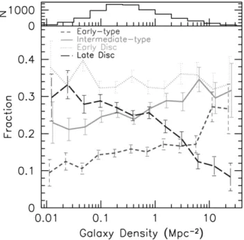
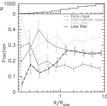
late (Sc) spirals. Figure 1.2 shows the correlation of morphological type with density. Specifically note that the fraction of late-type spirals increase towards low-density regions. In contrast, the percentage of early-type elliptical galaxies increase toward high-density regions. From Figure 1.3 we see evidence that the fraction of late-type galaxies increases with increasing clustercentric radius, while exactly the opposite relation holds for early-type galaxies. This morphology-density relation is consistent with a model in which spirals lose gas due to their motion through the intracluster medium and eventually are transformed into early-type galaxies (S0s).

Figure 1.2: Number fraction of galaxies of di↵erent morphology as a function of galaxy density (Goto et al. 2003).

1.3 Star Formation in Galaxy Clusters

Star formation in clusters of galaxies is one of the most complex process to understand in modern astrophysics. At the same time, it is one of the key ingredient that needs to be fully explored in order to obtain a more complete understanding of the evolution of galaxies. Quantifying star formation in high-density environments can also give us a clearer view of the dynamical processes that are at work inside of galaxy clusters. In

(23)

Figure 1.3: Galaxy morphology as a function of clustercentric radius. Distance has been scaled by the virial radius (Goto et al. 2003).

brief, the formation and evolution of a star is a balance between gravity and pressure. Star formation is directly a↵ected by the condition of the surrounding environment. Processes that compress star-forming gas or act to remove gas from individual cluster galaxies has a direct impact on galaxy evolution. Thus the study of star formation in galaxy clusters can be used as a diagnostic tool to probe the dynamical processes at work inside of high-density regions.

1.4 Classification of Galaxies

Although there are a number of ways of classifying galaxies, the Hubble tuning fork diagram is the most popular way of selecting galaxies based on morphological type (Figure 1.4).

(24)

Figure 1.4: The Hubble tuning fork diagram (image credit - ESA/Hubble). further subdivided into three sub-types based on the compactness of their spiral arms and relative brightness of their central bulges. Letters “a” to “c” are used to designate these sub-types, where “a” spiral galaxies have tightly wound spiral arms and bright bulges, and “c” types have loosely wound spiral systems and relatively faint bulges.

1.5 Dwarf Galaxies

The term dwarf galaxy is used to define galaxies of small intrinsic size, low luminosity, and faint surface brightness (Hodge 1971). The Large Magellanic Cloud is one of the most massive nearby dwarf galaxy (distance _⇠163,000 light-years). There are more than 20 dwarf galaxies in orbit around the Milky Way (Noyola et al. 2008). Many have been discovered in recent years using large area surveys. It is believed that some dwarf

(25)

galaxies are created by galactic tides as galaxies experience a tidal force under the influence of the more massive Milky Way gravitational field (Metz and Kroupa 2007). Dwarf galaxies are the most abundant type of galaxy in the Universe and are mostly found in galaxy groups and clusters. Due to their low luminosity, dwarf galaxies are in general difficult to detect. The demarcation between a dwarf galaxy and a more massive galaxy is typically defined using the absolute B-band magnitude. That is, dwarf galaxies are considered to be fainter than MB = 16. However, some studies

have adopted a di↵erent dividing line (Tolstoy and Murdin 2001). For example, the Small Magellanic Cloud (MB = 17) is considered a typical dwarf galaxy. The

average surface brightness of a dwarf galaxy is around 23 25 mag/arcsec2_.

Dwarf galaxies are classified into three main types; dwarf ellipticals, dwarf irregu-lars, and dwarf spheroids. Dwarf elliptical galaxies are very similar to normal elliptical galaxies, but smaller in scale. In general, they have little or no evidence of star forma-tion and are found to be on average metal poor. The mean mass of a dwarf elliptical galaxy is 107 _{to 10}9 _M _{, and with average diameters of 1 to 10 kpc. Luminosities} are on the order of 105 _{- 10}7 _L _{. Dwarf irregular galaxies lack organized structure} and thus are irregular in shape. They are normally gas rich, metal poor systems, and are very common among the Local Group of galaxies. A special sub-type of dwarf irregulars is the blue compact dwarf galaxies. These usually contain several compact high star-forming regions. NGC 1705 and NGC 1569 are examples of blue compact dwarf galaxies. Dwarf spheroidal galaxies on the other hand, do not contain a lot of gas, but show a complex star formation history. Some dwarf galaxies display episodic periods of star formation, which indicates that di↵erent types of dwarf galaxies may be a representation of di↵erent evolutionary stages (Tolstoy and Murdin 2001).

(26)

1.5.1 Star Formation in Dwarf Galaxies

Studies regarding the star formation in cluster dwarf galaxies are very limited in number. This is mainly due to the low luminosity and faint surface brightness of dwarf galaxies in nearby clusters. A large telescope is required for observing these systems. Star formation in dwarf galaxies have attracted attention in recent years due to their susceptibility to galaxy transformation processes in rich clusters. Simulations have shown that high speed encounters between galaxies inside rich clusters can transform disk galaxies into di↵erent types of dwarf galaxies (Moore et al. 1996). There is observational evidence for a diverse star formation history of nearby dwarf galaxies (Wright et al. 2018).

1.6 Indicators of Star Formation

There are various methods that have been used as indicators of star formation in galaxies. In particular, observations at ultraviolet, far infrared, radio, and H↵ wave-lengths have been employed.

1.6.1 Ultraviolet Observations

Ultraviolet (UV) wavelengths range from approximately 10 nm to 400 nm. Hot, young, massive O- and B-type stars are strong emitters of UV radiation. Due to this reason, UV is a strong indicator of recent star formation. The main advantage of UV is that it is directly related to the photosphere emission of a young stellar population. However, UV is strongly sensitive to extinction e↵ects due to dust. The Galaxy Evolution Explorer (GALEX) space telescope observed galaxies at UV wavelengths until 2012. One of the main goals of GALEX was to study star formation during the early stages of galaxy formation.

(27)

1.6.2 Far Infrared Measurements

A lot of the UV photons emitted by hot young stars is absorbed by interstellar dust. This heated dust re-radiates the energy mainly at wavelengths in the range of 10 to 300 µm, which is the far infrared (FIR). FIR observations can be used as an indirect measurement of star formation. The Infrared Astronomical Satellite (IRAS) was one of the earliest instruments used for FIR observations of star formation (Soifer et al. 1984).

1.6.3 Radio Continuum Detection

Radio emission from star forming galaxies has two components: thermal bremsstrahlung from ionized hydrogen, and non-thermal emission from spiraling electrons in a mag-netic field (synchrotron emission), usually associated with pulsars. However, radio emission is only an indirect measurement of the star formation rate (Bell 2003). De Jongl et al. (1985) has shown that there is a tight correlation between FIR lumi-nosity and radio emission of galaxies. Figure 1.5 shows this correlation for 91 galaxies with di↵erent morphological types (spirals and irregulars).

1.6.4 H

↵

Observations

H↵ observations are one of the fundamental methods of measuring star formation. As mentioned, hot young stars emit UV radiation. This emitted UV radiation is capable of ionizing hydrogen in the interstellar medium. When ionized hydrogen recombines with free electrons, H↵ photons corresponding to a wavelength of 656.3 nm are emitted as electrons transition between the n = 3 and n = 2 atomic energy

(28)

Figure 1.5: Relation between non-thermal radio emission ( = 6.3 cm) and far-infrared emission ( = 60µm) of 91 galaxies (de Jongl et al. 1985).

Figure 1.6: Emission of H↵ photons.

1.7 Galaxy Studies using

H

↵

Observations

There are a large number of observations specifically dedicated toH↵ measurements of galaxies. Some of these studies have focused specifically on cluster galaxies. Studies

(29)

that focus on the contribution of H↵observations to help understand star formation in galaxy clusters will be discussed here.

Kennicutt (1983) made the first attempt to measure the star formation rate (the total mass of stars formed per year) and equivalent width (EW; the measure of the area of a spectral line) for a large sample of galaxies. H↵ and red continuum fluxes of 170 nearby galaxies were used for this study, including both field galaxies and galaxies from the Virgo Cluster (Kennicutt and Kent 1983; Kennicutt 1983). This study found equivalent widths close to zero for ellipticals and S0 galaxies. These early-type elliptical galaxies typically consists of older stars, with little to no ongoing star formation. For late-type spirals, EWs were found to range from 20-50 ˚A and occasionally as high as 150 ˚A for some irregular and unusually active star-forming galaxies. This result is consistent with the general view that spiral galaxies have ongoing star formation. Kennicutt’s study is a good example of usingH↵ as a direct measurement of star formation rates.

Moss and Whittle (1993) observed eight nearby galaxy clusters using the Burrell Schmidt telescope at the Kitt Peak National Observatory (KPNO). The aim of this study was to compare star formation in cluster spiral galaxies with field galaxies. A total of 201 galaxies were observed of which 77 wereH↵emitting systems. Later, this group published a sample of 383 galaxies from the same survey (Moss and Whittle 2005).

Balogh et al. (2002) carried out an H↵ survey of A1689, a rich galaxy cluster at

z = 0.18. Spectra for 522 galaxies in the cluster were obtained (0.16< z <0.22) and strong H↵ emission was detected for 46 of these galaxies. Balogh et al. concluded that star-forming galaxies in the core of A1689 are significantly less in number than

(30)

This sample included 19 galaxy clusters observed with the Sloan Digital Sky Survey and available with the SDSS DR9 data release. More than 3000 galaxies with H↵ emission were observed.

The availability of large telescopes with modern detectors (CCDs) has improved our ability to detect fainter H↵ emitters in galaxy cluster environments. However, there is a lack of H↵ observations of dwarf galaxies in the cluster environment.

1.8 Initial Mass Function and Star Formation Rate

Properties of a star are directly related to mass. The initial mass of a star plays an important role as it determines the chemical and photometric evolution of galaxies. The number of stars formed in the mass interval (m, m+dm) and during the time interval (t, t+dt) is

(m)'(t)dmdt, (1.2)

where '(t) is the total mass of stars formed per unit time and (m) is a time-dependent function. The normalization constant can be found from (Schneider 2007),

Z 1

o

m'(m)dm = 1. (1.3)

'(t) is the star formation rate, while (m) is defined as the initial mass function (IMF). The IMF can be approximated by a power law and given by

'(m)_/m ↵. (1.4)

The IMF for stars greater than 1M can be approximated using↵ = 2.35. This form of the IMF is known as the Salpeter function (Salpeter 1955).

(31)

1.9 Redshift Dependence of Star Formation Rate

The density of the star formation rate (SFR) per comoving unit volume, ⇢SF R, is

measured in units of M yr 1_Mpc 3_{. Madau (1997) and his colleagues determined} the SFR at di↵erent redshifts. The “Madau diagram” is a plot of the SFR density as a function of redshift (see Figure 1.7). The Madau plot indicates a strong increase in the SFR density from the current epoch (z = 0) to z ⇡ 1, and a turnover for z > 1 up to z ⇡ 2. For redshifts greater than z ⇡ 3, ⇢SF R decreases. Recent observations

from the Spitzer and Herschel satellites have confirmed these results by observing a large sample of galaxies at FIR wavelengths.

Figure 1.7: Star formation density as a function of redshift (Madau 1997).

(32)

2007), ⇣ _M Ltot ⌘ ⇡300h⇣M L ⌘ . (1.5)

This value is about 10 times greater than the M/L for early-type galaxies (Schneider 2007). Zwicky (1937) addressed this problem by applying the virial theorem to the Coma Cluster and explained the “missing mass” by introducing dark matter. It is a well established fact that stars in galaxies contribute only about 5% of the total mass (normal + dark) in a cluster of galaxies.

Another important characteristic of galaxies in high-density environments is that two-body collisions in clusters are dynamically not important due to their large relax-ation time (estimated relaxrelax-ation times are much larger than the age of the Universe). Cluster galaxies also have nearly a constant velocity dispersion. Hence, violent relax-ation is dynamically more important for cluster galaxies to attain virial equilibrium (Schneider 2007). Violent relaxation is the process of the change in energy of indi-vidual mass particles due to the change in the overall gravitational potential of the cluster.

Dynamical friction is another important process that a↵ects the dynamics of galax-ies (Schneider 2007). If a massive particle of mass m moves through a homogeneous distribution of particles, the net gravitational force on particle m is zero due to the homogeneous distribution of other particles. But, particle m can attract other parti-cles, which will lead to an inhomogeneity in the distribution of surrounding particles behind particle m (i.e. a wake). The resulting overdensity of particles will follow the track of the massive particlem(Figure 1.8). This will decelerate particlemdue to the net force exerted by the overdensity of particles, thus acting like a frictiional force.

(33)

Figure 1.8: Schematic diagram of dynamical friction. Fd is the dynamical friction

force.

1.11 E

↵

ect of Cluster Environment on Galaxy Properties

As discussed earlier, the high-density cluster environment a↵ects the physical and morphological properties of cluster galaxies. Some of these e↵ects are discussed below.

1.11.1 Harassment

When collision speeds between galaxies in a cluster are higher than their internal velocity dispersions, no merging can take place. However, a collision can change the gravitational potential of one galaxy due to the flyby of another galaxy. This can increase the internal energy of matter. As a result, the matter can get heated and expand. This makes these galaxies less-bound gravitationally and more prone to changes by tidal forces. For example, the stellar disk of spiral galaxies can be

(34)

1.11.2 Cannibalism

The motion of a galaxy can be a↵ected by dynamical friction due to the cluster environment. As a result, the orbital semi-major axis of a galaxy will decrease over time by losing angular momentum and energy. Depending on gravitational friction and the mass of the galaxy, it can completely merge with the central galaxy of the cluster. Hence the central galaxy becomes more massive by cannibalizing other galaxy cluster members (Schneider 2007).

1.11.3 Ram Pressure Stripping

When a galaxy moves relative to the hot intracluster medium, the ICM acts as a wind in the rest-frame of the galaxy. This wind acts as a force on the interstellar medium due to the pressure from the ICM on the galaxy. If this force overcomes the gravitational restoring force of the galaxy, the gas can be removed from the host galaxy. This is known as ram pressure stripping and is believed to be one of the primary reasons for the morphology-density relation (Schneider 2007).

Since the ICM contains gas stripped from galaxies, the metallicity of the ICM is believed to be due to mixing of stripped gas from galaxies in the cluster. The efficiency of both ram pressure stripping and galaxy harassment depends on the orbit of the galaxy. The closer the orbits are to the center of the cluster, the greater the number density of galaxies, and hence the e↵ect of ram pressure will be larger. That is, for galaxies close to the cluster center, gas can be completely stripped away from the host galaxy, while only the loosely bound outer gas of a galaxy can be a↵ected for galaxies on larger orbits. For galaxies on larger orbits, the central region of a galaxy can continue to form stars until the gas is exhausted. Since the outer gas has already been removed due to ram pressure, no new gas can be gained and the galaxy will evolve passively and become red with no new star formation. This is known as

(35)

strangulation (Schneider 2007).

Butcher and Oemler (1978) found that a large fraction of blue galaxies exists in clusters at high redshift compared to low redshift (Butcher-Oemler e↵ect). The increase in the blue fraction is specific to the cluster environment. A possible expla-nation is that spirals lose gas over time through ram pressure stripping, which then gets mixed with the ICM. Thus lower redshift galaxy clusters are expected to have a smaller blue fraction compared to higher redshift clusters.

1.12 Objective

The main objective of this study is to quantify the impact of the high-density cluster environment on galaxies by measuring their star formation rate. Star formation rates will be measured by utilizing H↵ observations taken from the KPNO 4-m telescope with a CCD mosaic camera.

1.13 Theoretical Background

Gunn and Gott (1972) developed a theory to describe the infall of material into a galaxy cluster environment. If the temperature is high enough, the cluster en-vironment becomes smooth. Consider a cluster with a hot and smooth ICM. The interstellar matter of a galaxy that moves through the ICM will feel a ram pressure from the ICM. This ram pressure (Pr) is given by the following equation:

Pr ⇡⇢ICMv2, (1.6)

(36)

Fg = 2⇡G g s. (1.7)

Here g and s are the surface densities of stars and gas, and G is the gravitational

constant.

If Pr > Fg the galaxy will be stripped of its interstellar matter, which will lead

to a truncation or quenching of star formation. If Pr < Fg, the ram pressure will

not overcome the gravitational restoring force, and the interstellar matter will remain bound to the host galaxy. However, ram pressure could help to trigger star formation. McCarthy et al. (2007) derived an analog model for ram pressure stripping.

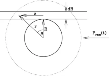
As-Figure 1.9: A schematic diagram of ram pressure stripping for a spherically symmetric gas distribution (McCarthy et al. 2007).

suming that the loosely bound outer gas of a galaxy is more likely to be stripped away due to ram pressure, one can writedA = 2⇡RdR for the annulus in Figure 1.9. This is the projected area of the annulus. The force due to ram pressure can be written as

Fr =PrdA. IfFr > Fg, the gas in the annulus will be stripped away toward the

oppo-site direction of v (z-direction in Figure 1.9). If the maximum restoring acceleration and the gas density of the annulus are given bygmax(R) and g(R), the condition for

(37)

ram pressure stripping is

⇢ICMv2 > gmax(R) g(R). (1.8)

1.13.1 Observational Evidence of Ram Pressure Stripping

A recent observation of ESO 130-001, a galaxy in the Abell 3627 cluster, shows clear evidence for ram pressure stripping (Figure 1.10).

Figure 1.10: Left: XMM-Newton 0.5-2 keV image of the A3627 cluster. The main tail of ESO 137-001, due to ram pressure stripping, is clearly visible. Right: Composite image of X-ray,H↵, and optical observations of galaxyESO130 001 in A3627 (Sun et al. 2009).

The blue color tail trailing behind the galaxy represents X-ray emission observed from the Chandra X-ray observatory. Optical emission is denoted by the yellow color, while the H↵ emission is red. The optical and H↵ data are obtained from the Southern Astrophysical Research (SOAR) telescope in Chile. The X-ray tails are created when cool gas is stripped away from the galaxy as it travels towards the center of the cluster. The H↵ data indicates star formation. This is the first direct

(38)

The galaxy NGC 4402 shows evidence of ram pressure stripping (Figure 1.11). NGC 4402 is currently falling into the Virgo Cluster. The dust and gas disk of the galaxy appears to be bowed, which indicates that the galaxy is loosing gas in its outer region due to external pressure. The blue stellar disk also appears to extend away from the star-forming disk. These observations provide strong evidence to show that gas in the outer regions of the galaxy is being stripped away. A stream of dust is also found to be trailing behind the galaxy.

Figure 1.11: NGC 4402 falling towards the Virgo Cluster (downward direction of the image: http://astronomy.swin.edu.au/cosmos/R/Ram+Pressure+Stripping).

1.14 Outline

In order to measure star formation rates of cluster galaxies for this study, continuum images are subtracted from H↵ observations. Images observed using a narrow-band filter centered on the redshifted H↵ emission line will contain both line emission plus continuum. A broad-band filter image of the same area contains mainly the continuum emission. By properly scaling and subtracting the broad-band image from the narrow-band image, the H↵ emission flux can be extracted. Corrections are required for internal and external extinction, which are discussed in the chapters on

(39)

data reductions and analysis.

The Picture Processing Package (PPP; Yee 1991) will be used for object finding, photometric measurements, and star-galaxy classification. The measured H↵ flux from cluster galaxies will be used to estimate star formation rates.

(40)

Chapter II

OBSERVATIONS

Ther-band andH↵ observations used in this study were obtained from the Mayall 4-meter telescope at the Kitt Peak National Observatory (KPNO). The 4-m telescope is the largest optical reflecting telescope at KPNO and is located just below the summit of Kitt Peak at 6875 feet. Historically, the Mayall 4-m telescope has played an important role in uncovering evidence for dark matter through observations of flat rotation curves in galaxies (De Blok et al. 2001).

The light gathering power (LGP) of a reflecting telescope is depended upon the diameter of the primary mirror, and is given by the following relation:

LGP _/D2, (2.1)

where D is the diameter of the telescope primary mirror.

The di↵raction limit of a telescope depends on both the diameter of the primary mirror (assuming a circular mirror) and the observed wavelength. The angular sepa-ration (✓min) at which two adjacent light sources are just barely resolved is given by

the Rayleigh criterion (Carroll and Ostlie 2007):

✓min = 1.22

D, (2.2)

where is the wavelength and D is the diameter of the primary mirror. Thus the larger the size of the mirror in a reflecting telescope, the greater the ability to detect faint objects and resolve finer details.

(41)

Figure 2.1: KPNO 4-m telescope.

2.1 Mosaic Imagers

The Mosaic-1.1 imaging camera was used for the first two observing runs at KPNO. This detector consists of eight 2048⇥4096 pixel CCD chips arranged as a 8192⇥8192 pixel detector, a filter track with a capacity to hold 14 filters, two intensifier CCD TV cameras, and four electronic array controllers (ARCONs; Muller et al. 1998). To achieve a faster read-out time, the imager contains sixteen amplifiers (two per CCD chip). The CCD chips are separated by a 1.2 mm gap, which is equivalent to 80

(42)

Image Size 8192_⇥8192 pixels

Pixel Size 15µm

Read Noise 5.9e

Dark Current 4.4e /hour

CCD Gaps 1.2 mm= 80 pixels in both row and column

Gain 1.2 e/ADU

Linearity Up to the saturation Level Saturation level 218,000 e

Field of View 360_⇥₃₆0

Table 2.1: Properties of Mosaic 1.1.

camera2_{. This detector has four CCD chips with four amplifiers per chip. The basic} properties of this camera are given in Table 2.23_{. Both cameras have great sensitivity} for acquiring the needed observations for this study (i.e. ⇡ 80% quantum efficiency in the r-band).

The CCD detectors output data as multi-extension Flexible Image Transportation System (FITS) files. The display orientation of the Mosaic-1.1 and Mosaic-3 cameras are shown below.

Figure 2.2: CCD orientation of Mosaic-1.1.

2_{https://phys.org/news/2016-02-galaxy-hunting-sky-camera-redder.html} 3_{https://www.noao.edu/kpno/mosaic/manual/}

(43)

Image Size 8448_⇥8448 pixels

Pixel Size 15µm

Read Noise 8e

Dark Current 0.95 e /hour

CCD Gaps 200 pixels in Dec and 240 pixels in RA

Gain 1.8 e/ADU

Linearity Up to the saturation level Saturation Level 35,000 e

Field of View 360 _⇥₃₆0

Table 2.2: Properties of Mosaic-3.

Figure 2.3: CCD orientation of Mosaic-3.

(44)

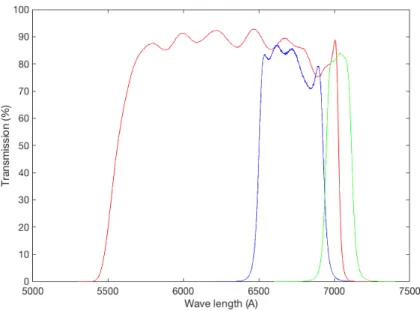
located within our available narrow-band filter bandpass. The r-band filter (K1018) was used to observe the continuum, while the Windhorst BATC 666 (k1059) and Windhorst BATC 705 (K1060) narrow-bandH↵ filters were used for observations of the redshifted emission line. The width of the r-band filter is given as the full width at half maximum (FWHM) of 1475.17 ˚A, and has a maximum transmission of 92.83% at a central wavelength of 6465 ˚A (Figure 2.4). The K1059 and K1060 narrow-band filters have a maximum transmission of 87.5% and 87.8%, respectively. The K1059 filter width has a FWHM=430.58 ˚A, while the K1060 filter has a width of 177 ˚A (see Figures 2.5, 2.6, and 2.7).

(45)

Figure 2.5: Filter transmission curve for the K1059 filter.

(46)

Figure 2.7: Narrow-band filter transmission curves compared to the broad-band filter. The broad-band filter (r) is shown by the red color, while the blue and green colors represents the K1059 and K1060 narrow-band filters, respectively.

2.3 Observing Conditions

The KPNO is located at a high elevation and far from the nearest city of Tuscon. The distance from Tucson and its strict by-laws regarding light pollution, makes KPNO a good site for conducting astronomical observations of faint objects. KPNO is also known for its good seeing (Carroll and Ostlie 2007), where seeing is a measurement of the blurriness of a star-like object due to the Earth’s atmosphere.

A total of two half-nights of observations were awarded for the first observing run on the 4-m telescope. Out of these two half-nights, data from the first half-night was not used due to poor seeing conditions. The average seeing for the second night was 1.500_{. The second observing run consisted of three half-nights with an average seeing}

of 1.500_{. The third and final observing run consisted of three full nights using the}

newly installed Mosaic-3 imager. Out of three full nights, one night was lost due to bad weather. The first night had excellent seeing of 100, while for the second night the average seeing was 200.

(47)

2.4 Galaxy Cluster Sample

A total of 12 galaxy clusters was observed during the combined three observing runs. Observations were carried out on February 11-12, 2015 and June 12-14, 2015 using the Mosaic-1.1 imager. The third observing run took place on January 29-31, 2016 using the Mosaic-3 detector. The galaxy cluster sample was selected to have a redshift range of 0.03 < z < 0.15 so that clusters were close enough so that star-forming dwarf galaxies could be sampled in a reasonable exposure time. The clusters were also selected so that they were observable from KPNO during the awarded observing time, and that the redshifted 6563 ˚A H↵ emission line was centered on one of the available narrow-band filters. Of the 12 observed clusters, two clusters were omitted from the final sample due to bad seeing. Thus a final sample of 10 galaxy clusters was available for analysis for this study (Table 2.3 and Figure 2.8).

For the Mosaic-1.1 camera, each cluster was observed for 300 seconds per pointing using the r-band filter, and 600 seconds for the narrow-band H↵ filter. In order to compensate for chip gaps, bad pixels, and cosmic rays, each cluster was observed using a standard five-point dither pattern4_{. This resulted in a total integration time} per cluster of 5_⇥300 seconds for the r-band filter and 5_⇥600 seconds for the H↵ filter. Due to the high sensitivity and low saturation level of the Mosaic-3 camera, exposure times of 300 seconds per pointing for ther-band filter and 450 or 600 seconds (depending on the cluster redshift) for the H↵filter was used with the standard five-point dither pattern.

(48)

Cluster RA Dec Filters Redshift A426 03:19:46.99 +41:30:47.16 r/k1059 0.018 A496 04:33:38.40 -13:15:33.00 r/k1059 0.033 A576 07:21:24.10 +55:44:20.00 r/k1059 0.039 A757 09:12:47.29 +47:42:38.00 r/k1059 0.052 A1569 12:36:18.70 +16:35:30.00 r/k1060 0.073 A1691 13:11:11.14 +39:16:38.40 r/k1060 0.072 A1983 14:52:44.00 +16:44:46.00 r/k1059 0.044 A2063 15:23:01.79 +08:38:21.98 r/k1059 0.035 A2107 15:39:47.90 +21:46:21.00 r/k1059 0.041 A2147 16:02:17.20 +15:23:43.00 r/k1059 0.035

Table 2.3: Observed galaxy cluster sample.

Figure 2.8: Spatial distribution of observed galaxy clusters.

2.5 Calibration Frames

For each observing night, seven flat field images were taken with each filter. This process was done by pointing the telescope at a uniformly illuminated screen inside of the observatory dome. The illumination of the flat field screen was achieved by using appropriate voltage settings of flat field lamps so that the flat field images had a high signal-to-noise (S/N) without approaching the saturation level of the detector. Eleven bias frames were taken for each night using zero-second exposures (i.e. with a closed shutter). Dark frames were not observed since the dark current for the

(49)

two detectors is negligible (Tables 2.1 and 2.2). The importance of these calibration frames is discussed in the data reduction section of Chapter III.

(50)

Chapter III

DATA REDUCTION

3.1 Introduction

Images acquired using the Mosaic-1.1 and Mosaic-3 imagers were stored in the FITS format. The FITS format is a standard file format used at most professional ob-servatories. This format allows data to be stored, transmitted, and processed as N-dimensional arrays (e.g. a 2D image). The FITS format allows the storage of images with an ASCII header that typically includes photometric, astrometric, and calibration information (e.g. right ascension, declination, exposure time, filter details, etc.).

Due to the large field-of-view of both the Mosaic-1.1 and Mosaic-3 cameras, data reduction was a tedious task. Since the Mosaic-3 camera was just installed prior to the final observing run, most of the standard calibration files were not available. Calibration files for Mosaic-3 (e.g. crosstalk coefficients and WCS database files) had to be created. The data reduction steps are explained in detail in this and subsequent chapters. In summary, there are four major steps in data reduction: photometric calibration, astrometric calibration, PSF (point spread function) matching for proper image subtraction, and making of the final object catalog. For this study the Image Reduction and Analysis Facility (IRAF) software was used for image processing.1

(51)

3.2 CCD Operation

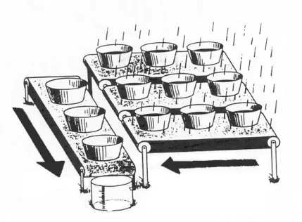
A simple way to understand the operation of a CCD is to use the water bucket analogy (Howell 2006). Each pixel in a CCD is represented by a bucket and incoming photons can be considered as rain drops. A field covered with buckets aligned into rows and columns (Figure 3.1), can collect raindrops during a rain storm (equivalent to the integration time for a CCD observation). Each bucket is then transferred and measured to determine the amount of water collected. The final record of the amount of water collected in each bucket is equivalent to the output of CCD pixels in an image.

Figure 3.1: Water bucket analogy of CCD operation. Each bucket represents a pixel in the CCD chip (Howell 2006).

The physics behind CCDs is based on the photoelectric e↵ect. Atoms in a semi-conductor such as silicon are arranged in discrete energy bands. The lower energy band, the valance band, is occupied by most of the electrons. Incoming photons are

(52)

storing a certain number of electrons (the full-well capacity of the CCD) until the end of the integration. At the end of the exposure time, each pixel row is read out in parallel through a shift register (this is equivalent to the three lower level buckets in Figure 3.1). Once an entire row is shifted into the output register, each pixel is shifted again to the output electronics and measured as a voltage. This voltage is amplified by a low noise on-chip amplifier and converted to a digital number (analog-to-digital unit or ADU) using an analog-to-digital (A/D) converter. ADUs are also referred to as counts and is the primary unit of brightness measured in FITS image display programs. The number of electrons required to produce 1 ADU is defined as the gain of the CCD. Read-out time of a CCD depends on the speed of the A/D conversion. Modern large format CCDs use two or more amplifiers to obtain a faster read-out time.

3.3 Instrumental Calibrations

The data reduction procedure for processing images from mosaic cameras is more complicated than that used for single-chip CCD detectors. This is due to the fact that the Mosaic-1.1 and Mosaic-3 imagers consists of four CCD chips, with each chip read out through several amplifiers. Hence, each FITS image read to the computer is a multi-extension FITS file (i.e. a seperate extension for each amplifier). Since each image contains 16 extensions, mosaic images are not directly readable through normal FITS file readers such as DS9.2 _{The IRAF software system is used for most} of the data reduction steps since it is capable of handling multi-extension FITS files through the MSCRED package.

(53)

3.3.1 Crosstalk Calibration

Since each amplifier is read out in parallel, a signal in one amplifier may a↵ect the sig-nal in another amplifier. This is known as crosstalk. The crosstalk from one amplifier to another can be seen as a ghost image or the faint artifact of a bright star. Theo-retically, the crosstalk e↵ect occurs at all signal levels, but is only visible for bright sources. This e↵ect needs to be corrected for prior to other standard calibrations. IRAF has two separate tasks to find the crosstalk coefficients (XTCOEFF) and apply the correction to images (XTALKCOR).XTALKCORand XTCOEFFuse the crosstalk model proposed by James Rhodes (Valdes 2002). During the calibration process, a crosstalk coefficient between the source amplifier and the victim amplifier was determined, and then the source image was multiplied by the relevant coefficient. The source image is responsible for creating the crosstalk signal on the victim image. A source image can be a victim, and a victim image can be a source as well. Calculated crosstalk coefficients are available for the KPNO Mosaic-1.1 camera,3 _{but were not available} for the Mosaic-3 detector. Hence XTCOEFF and equation 3.1 were used to calculate the crosstalk coefficients:

↵vs =

(Iv B)

Is

, (3.1)

where Is is the source pixel value, Iv is the matching victim pixel value, B is the

background estimator for the read-out line, and↵vs is the calculated crosstalk coeffi

-cient for each pixel. The set of coefficients from individual pairs were fit to a constant function to remove outliers, where the fitted constant (or average) is the crosstalk coefficient for the amplifier. The average coefficient was applied to each pixel from

(54)

Figure 3.2: A section of the A426 r-band cluster image before (left) and after (right) applying the crosstalk correction.

3.3.2 Pupil Ghost Correction

A pupil ghost image was visible in most of the observed images, including the flat field frames. This is a known issue for the KPNO 4-m telescope (Jannuzi et al. 2003; Valdes 2002), and the exact reason is subtle. Jacoby et al. (1998) states that light passing through the prime focus corrector of the telescope returns back to the primary mirror and get reflected back again to the detector to produce the ghost image. The pupil ghost image was visible in flat field images as a bright ring at the middle of the image frame. The intensity of the ghost image depends on the filter bandpass (Jannuzi et al. 2003) and is inversely proportional to the width of the filter (i.e. more prominent in narrow-band images).

Since this is an additive e↵ect, flat field images were corrected before applying them to the relevant science images. The pupil ghost correction preserves the pixel-to-pixel variations of the flat field images. The pupil pattern is modeled as a ring and subtracted from the original flat field images. The IRAF task MSCPUPIL was used to model the ring by fitting a function using polar coordinates (r,✓; see Figure 3.3).

3.3.3 Bias and Flat Field Calibrations

Bias frames were taken with zero second exposures (i.e. closed shutter) to determine the underlying electronic noise level in each data frame. The bias signal is a spatial frequency variation of the CCD image due to the CCD on-chip amplifiers (Howell

(55)

Figure 3.3: Raw flat field image with pupil ghost (left), and the corrected flat field image using MSCPUPIL(right).

2006). A 2D pixel-by-pixel subtraction was needed to remove the bias level from the science images. Since a single bias frame does not sample these variations adequately, 11 bias frames were taken and averaged together to make a final ‘master’ bias frame per night.

Each pixel in a CCD chip responses di↵erently to light and thus each pixel will have a di↵erent wavelength-dependent gain. Flat field images were used to remove this pixel-to-pixel variation in sensitivity. Each science image for each filter was divided by an averaged nightly master flat field image, which was constructed by averaging together seven dome flat field images per filter per night. The combined calibration of bias subtraction and flat field correction is summarized in equation 3.2:

Corrected image = Raw image Bias F rame

Corrected F lat F ield image, (3.2)

where the corrected flat field image has the pupil ghost removed. No attempt was made to remove the pupil ghost from the science images that were bias-corrected and

(56)

Figure 3.4: The central section of the A426 r-band image before (left) and after (right) applying bias and flat field corrections.

3.3.4 Sky Flat Field Correction

The basic flat field correction described previously is not adequate for mosaic images. This is due to several reasons: 1) CCDs in a mosaic camera must be brought to the same gain level in order to preserve the ADU counts for a given exposure time, 2) the non-uniformity of the illumination of the large field-of-view of the mosaic imager from the flat field lamps (Valdes 2002), and 3) the color mis-match between the dome flat field images and the night sky (Valdes 2002). The first stage of flat fielding using dome flats allows for the di↵erentiation between scattered light patterns and the pixel-to-pixel response variation. The second stage is the application of a “sky flat” to the existing dome flat field-corrected images. The sky flat accounts for the color di↵erence between the night sky and the dome flat field lamps used for the initial flat fielding step.

To make a sky flat field image, the IRAF task COMBINE was used to combine all science (cluster) frames for a given filter by first rejecting all object pixels above a certain brightness threshold using an average sigma clipping algorithm. The images

(57)

were then median combined to make a “master” sky flat field image for each filter for a particular observing run (see Figure 3.5).

Figure 3.5: An r-band median combined sky flat field image. A total of 22 cluster frames from two nights of observing were used in the construction of the flat field image.

Finally, the CCDPROC task in IRAF was used to apply the sky flat field image to each science frame. This step completes the basic instrumental calibration process for all science images.

3.3.5 Final Calibrated Images

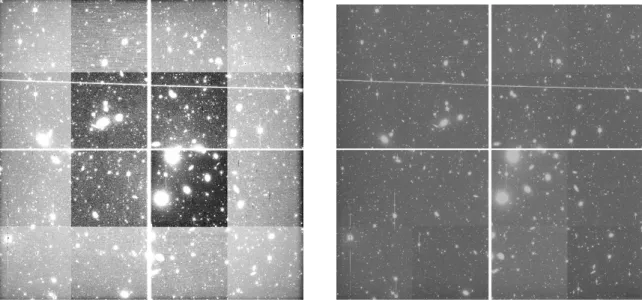
Figures 3.6 and 3.7 show the di↵erence between the pre-processed (raw) and post-processed r-band image of the galaxy cluster A2107.

(58)

(59)

Figure 3.7: Image of A2107 cluster, observed using the r-band filter, after applying the bias and flat field calibration steps.

3.4 Astrometric Calibration

Accurate astrometric calibration plays a major role when combining di↵erent CCD mosaic images into a single extension FITS file. Each CCD image has its own mapping function that details the rotation, scale, and optical distortions specific for that CCD. Since the goal is to stack a set of dithered images (i.e. each image is shifted by a small amount to fill in chip gaps, etc.) to obtain a final deep image, having accurate

(60)

3.4.1 World Coordinate System

The goal of astrometric calibration is to refine the world coordinate system (WCS) by accurately mapping pixels on a CCD to celestial coordinates on the sky (e.g. right ascension and declination). There are 16 extensions in one mosaic image, and each extension requires its own WCS in order to correct for relative orientations of the CCDs and optical distortions. Images obtained with the KPNO mosaic cameras contain default WCS information using several header keywords such as WCSDIM, CTYPE1, CTYPE2, CRAVL1, CRVAL2, CRPIX1, and CRPIX2. WCSDIM gives the dimensionality of the WCS, and is equal to two when dealing with two dimensional images. CTYPE1 and CTYPE2 are used to describe the projection used for the right ascension and declination coordinate system. The projection is how images are mapped onto the sky. For mosaic images, the usual projection method is the tangent plane projection. This is a fairly accurate representation considering that the CCD surface is a small flat square that is projected onto a particular point on the celestial sphere. CRPIX1 and CRPIX2 are coordinates of the tangent point where the CCD is positioned on the celestial sphere. CRVAL1 and CRVAL2 are the corresponding coordinates on the celestial sphere. The rotation matrix (see equation 3.3) describes how CCD pixels translate to astronomical coordinates, and how the CCD image is rotated relative to the axes of the celestial sphere:

R = Cos ✓ Sin ✓

Sin ✓ Cos ✓

. (3.3)

Equation 3.4 describes the transformation of CCD pixel coordinates to celestial coordinates:

(61)

wherea= (RA CRVAL1,DEC CRVAL2) andu= (x CRPIX1,y CRPIX2). a

and u are vectors of the celestial and pixel coordinates relative to the tangent point,

s is the angular size of a pixel, and R is the rotation of the CCD image relative to celestial North.4

3.4.2 WCS Calibration Process

For mosaic images, WCS information is stored in the image headers when the data are transfered from the detector to the data acquistion computer. In addition, KPNO provided a WCS database file that contains information required to update the WCS in each mosaic image. It is generally assumed that the WCS function is static. That is, once the WCS is determined for a particular point on the sky, it can be translated to other positions using di↵erent rotation angles on the sky (Valdes 2002). Thus a global calibration file is enough to update the coordinate system of any image taken from a particular mosaic camera.

For the Mosaic-1.1 camera, a WCS calibration file was provided and theMSCSETWCS

task in IRAF was used to load accurate WCS information into the image headers. Since the Mosaic-3 imager was newly installed in February 2016, only initial WCS calibration files were provided by KPNO. A check of these calibration files using the FITS image display tool DS9 showed that some of the RA and Dec coordinates were not accurate. In particular, galaxy clusters A757, A426, and A576 had WCS errors in both translation and rotation relative to the standard USNO-A 2.0 astrometric ref-erence catalog. To correct for this, WCS coordinates for these images were improved by creating a new WCS database file.

4

(62)

3.4.3 WCS Calibration Improvements for Mosaic 3.0 Images

The MSTPEAK task in IRAF was used to generate a new global WCS calibration file,

which was applied to the images that had inaccurate coordinates. The output of this task is a WCS solution for each amplifier and can be applied to each mosaic image using the IRAF task MSCSETWCS. This task is capable of reading astrometric information from a standard reference catalog, and calculate rotations and shifts for each amplifier in a CCD mosaic image by interactively fitting the data. The initial WCS positions of image objects were used as a starting point. A tangent plane projection and a third-order polynomial fit (for non-linear corrections) were used to calibrate the WCS.

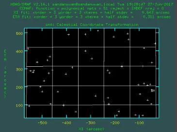
First, MSCTPEAK was used to display an image, and the initial WCS object posi-tions were marked by red circles (see Figure 3.8). These objects were selected from the standard astrometric reference catalog (e.g. USNO-A 2.0). The correct WCS positions were then marked for some of the objects and positions of other objects were adjusted using cursor keys5_{. Once the correct objects were marked, a new WCS} calibration was applied to the image and x- and y-residual plots were checked for accuracy. This process was repeated until an accurate WCS fit was obtained. It was also important to make sure that selected objects for the fit were distributed spatially over the whole image to help ensure an accurate WCS solution.

(63)

Figure 3.8: WCS positions of objects in the A757 cluster field for one amplifier. Red circles are the original WCS positions and the blue circles are for the corrected WCS coordinates.

Figure 3.9: Spatial distribution of selected catalog objects from A757 for WCS cali-bration.

(64)

Figure 3.10: X-coordinate fit residuals for objects in A757.

Figure 3.11: Y-coordinate fit residuals for objects in A757.

3.4.4 Final Corrections to WCS

Once the correct WCS calibration is applied to all images, small corrections using the task MSCCMATCH in IRAF can be used. The task MSCGETCATALOG is called

in-side MSCCMATCH so that it automatically downloads the USNO-A 2.0 catalog from a

Web-based server and uses it to make WCS corrections to the mosaic images. The downloaded catalog is a simple text file containing accurate right ascension and dec-lination coordinates for a set of objects within a defined magnitude range for a given

(65)

cluster image. The most important aspect of this task is the pattern matching algo-rithm. Objects in the astrometric catalog are matched to positions of objects in a cluster image. A global linear correction is then applied depending on the di↵erence between the catalog object positions and the corresponding object positions in the cluster image. Since this is an automated task, it is important to have an accurate WCS for all images so that only a small shift and rotation correction is required. The

MSCCMATCH task is run interactively using a large number of objects across an image field in order to fine-tune the WCS calibration.

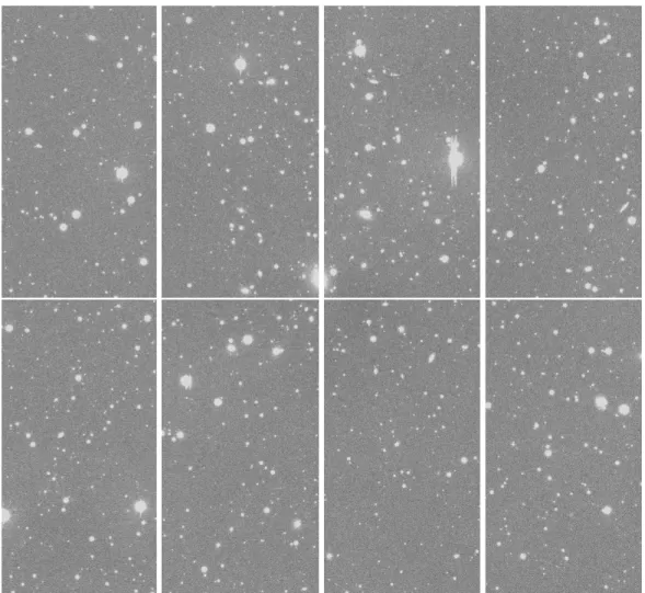
3.5 Construction of Single Cluster Images

All steps up to now have been applied using the KPNO mosaic MEF images. These images need to be converted to single extension FITS files before being stacked to-gether to form a single deep cluster image. This step is straight forward if all MEF images have an accurate WCS. The IRAF task MSCIMAGE was used to merge all 16 image extensions from the 16 amplifiers to construct a final single-extension FITS image (Figure 3.12).

Exploring Star Formation In Cluster Galaxies

University of North Dakota

UND Scholarly Commons

Exploring Star Formation In Cluster Galaxies

Sandanuwan Prasadh Kalawila Vithanage

EXPLORING STAR FORMATION IN CLUSTER

GALAXIES

Permission

TABLE OF CONTENTS

LIST OF FIGURES

LIST OF TABLES

Acknowledgements

Dedications

ABSTRACT

Chapter I

INTRODUCTION

1.1

Galaxy Clusters

1.1.1

Morphological Classification of Galaxy Clusters

1.2

Galaxy Population in Clusters

1.2.1

Luminosity Function

1.2.2

Morphology-Density Relation

1.3

Star Formation in Galaxy Clusters

1.4

Classification of Galaxies

1.5

Dwarf Galaxies

1.5.1

Star Formation in Dwarf Galaxies

1.6

Indicators of Star Formation

1.6.1

Ultraviolet Observations

1.6.2

Far Infrared Measurements

1.6.3

Radio Continuum Detection

1.6.4

H

↵

Observations

1.7

Galaxy Studies using

H

↵

Observations

1.8

Initial Mass Function and Star Formation Rate

1.9

Redshift Dependence of Star Formation Rate

1.11

E

↵

ect of Cluster Environment on Galaxy Properties

1.11.1

Harassment

1.11.2

Cannibalism

1.11.3

Ram Pressure Stripping

1.12

Objective

1.13

Theoretical Background

1.13.1

Observational Evidence of Ram Pressure Stripping

1.14

Outline

Chapter II

OBSERVATIONS

2.1

Mosaic Imagers

2.3

Observing Conditions

2.4