Working Paper Series
2013-03
Dos and Don‘ts of Gini
Decompositions
November 2013
Simon Jurkatis, Humboldt-Universität zu Berlin
Wolfgang Strehl, Freie Universität Berlin
Sponsored by BDPEMS
Spandauer Straße 1 10099 Berlin
Tel.: +49 (0)30 2093 5780 mail: [email protected]
Dos and Don’ts of Gini Decompositions
Simon Jurkatis
∗,a,cand Wolfgang Strehl
b,caHumboldt-Universit¨at zu Berlin bFreie Universit¨at Berlin
cBerlin Doctoral Program in Economics & Management Science
November 15, 2013
Abstract
This paper critically assesses widely applied methods of Gini de-composition by income sources and population subgroups. We point to common pitfalls in the interpretation of decomposition results and show that marginal effects provide the only meaningful way to exam-ine the relevance of income sources or population subgroups for total income inequality. Moreover, we show that existing methods are
un-suitable to decompose thetrend in the Gini coefficient, i.e. to examine
the role of income sources or population subgroups for the change in the Gini over time. We provide a coherent method to decompose the Gini trend by income sources.
Keywords: Income inequality; Gini decomposition; Income sources; Population subgroups; Inequality trend
JEL classification: C43, D31, D33, D63, O15
∗Corresponding author. E-mail: [email protected]. Tel.: +49 (30) 838 53240.
We thank Philipp Engler, Holger L¨uthen, Dieter Nautz, Shih-Kang Chao and Georg Weizs¨acker for helpful comments and suggestions. We also thank Srikanta Chatterjee and Nripesh Podder for valuable discussions.
1
Introduction
“. . .the disaggregation of the Gini coefficient is probably the most misused and misunderstood concept in the income inequality lit-erature.”
(Podder and Chatterjee, 2002, p. 3) Judging from the number of references in the inequality literature, the most prominent measure of income inequality is the Gini coefficient dating back to Corrado Gini (1912). Since then, the Gini has been used extensively in a still growing literature that examines how income inequality spreads over income sources and population subgroups, and how it develops over time. For these purposes the Gini has been decomposed in numerous ways. Yet, despite the Gini’s long existence, mistakes continue to be made when it comes to the interpretation of Gini decomposition results, and misleading methods of decomposition do not stand corrected. As the above quote by Podder and Chatterjee (2002) suggests, the misuse and misinterpretation of Gini decompositions is well known to the literature. Unfortunately, however, neither Podder and Chatterjee (2002) nor subsequent studies could finally resolve the issues regarding the Gini decomposition. The consequences of misinterpretations or misleading methods cannot be overstated, as Gini de-composition results may be used by policymakers to understand underlying trends in the distribution of income and, most relevantly, to assess differ-ent tax and transfer policies in terms of their effectiveness to reduce overall income inequality.1
Against this background, our contribution is to show which questions can and cannot be reasonably addressed within the Gini decomposition
frame-1To give one example, falsely attributing an increase in inequality, as measured by the
Gini coefficient, to changes in the distribution of capital income, as opposed to changes in wage income, may lead to wrong conclusions about redistributional measures enacted in the past and/or to misdirecting policy recommendations to counteract the increase in inequality.
work. We will briefly review the traditional methods of Gini decomposi-tion by income sources and populadecomposi-tion subgroups and then critically assess some subsequent methodological advances that took place in response to the caveats of the traditional approaches. We show that these advances, in turn, are subject to various shortcomings and propose, where possible, ways to overcome these.
In Section 2, we discuss the well-established Gini decomposition by in-come sources, originally proposed by Rao (1969), and the transformation thereof proposed by Podder (1993b). The objective of these decomposition methods is to assess the importance of an income source, e.g. capital in-come or government transfers, for total inin-come inequality. To that end, the traditional method of Rao (1969) disaggregates the Gini into the income sources’ so-called concentration coefficients2 and weights these coefficients
by the share of the respective income source in total income. We will briefly recapitulate that unfortunately, however, the traditional method suffers from a non-interpretability of the decomposition results (Shorrocks, 1988) and the violation of the property of uniform additions (Morduch and Sicular, 2002). Motivated by the latter, Podder (1993b) proposes a transformation that cir-cumvents this violation and, moreover, is supposed to yield interpretable results. In particular, Podder (1993b) and Podder and Chatterjee (2002) claim that the transformation allows assessing whether the presence of an income source (or the absence thereof) increases or decreases total income inequality. Yet, we show that the results obtained from Podder’s (1993b) transformation do not allow drawing such conclusions. In fact, one cannot even deduce whether the absence of an income source that is concentrated— more than any other income source—in the upper region of the income dis-tribution would decrease or increase total income inequality. Instead, we find that the transformation by Podder (1993b) is informative about the effect
2Roughly speaking, a concentration coefficient measures the relation of an income
source with the rank of its recipients in total income, i.e. it indicates whether an in-come source accrues mainly to relatively poor or rich households.
of marginal changes in an income source as it is closely linked to the elas-ticity of the Gini coefficient with respect to the mean of an income source. We arrive at the conclusion that only these elasticities (also referred to as marginal effects) allow for a meaningful assessment of the effect of an income source on total income inequality as they provide a quantitative, as well as an unambiguously interpretable assessment.
We end Section 2 by addressing the decomposition of the trend of the Gini coefficient which aims at explaining the change in the Gini in terms of changes in income sources over time. We argue that the approaches put forth in the literature (Fei et al., 1978; Podder and Chatterjee, 2002) are unsuitable to provide this insight and establish an approach that fills this gap. Intuitively, changes in an income source over time can contribute to an increase in the Gini in two different ways: first, if the distribution of that income source changes in favor of relatively rich individuals (or households); second, if the share of that income source in total income increases while at the same time the distribution of the income source is more in favor of relatively rich individuals than that of total income (or, conversely, if the income share of that source decreases while its distribution is less in favor of relatively rich individuals than that of total income). We show that this latter comparison of the distribution of an income source with the distribution of total income is missing in the approach of Podder and Chatterjee (2002) which causes their method to be in contradiction to the abovementioned Gini elasticity. Fei et al. (1978), on the other hand, base their approach on a pairwise comparison of the distributions of the income sources, which captures implicitly the two effects described above, but makes their method less feasible the more total income is split into different sources.
In Section 3, we turn to the Gini decomposition by population subgroups which aims at explaining total income inequality in terms of the income of different population subgroups.3 The traditional approach of Bhattacharya 3A population may be grouped along ethnical, geographical, religious, generational etc.
and Mahalanobis (1967) gives rise to an overlapping term, which impedes the applicability of this method (Cowell, 2000; Mookherjee and Shorrocks, 1982). Here we will thus focus on an alternative decomposition method pro-posed by Podder (1993a), which has been recently reasserted by Chatterjee and Podder (2007). The method is in a similar fashion as the decomposition by income sources of Rao (1969) referred to above, i.e. it disaggregates the Gini into the income shares and concentration coefficients of population sub-groups, and has the particular advantage of the absence of the overlapping term.4 Yet, we stress that the method does not come without drawbacks. We
first show that the decomposition results do not allow inferring—as suggested by Podder (1993a) and Chatterjee and Podder (2007)—whether the presence of the income of a subgroup increases or decreases total income inequality. Second, we highlight that the ability of this decomposition method to explain
changes in the Gini coefficient in terms of the underlying changes in popula-tion subgroups is severely limited as changes in the concentrapopula-tion coefficients cannot be mapped unambiguously to changes in the population subgroups. We show that this failure can lead to highly misleading conclusions.5 Finally,
we stress that marginal effects (in terms of the Gini elasticity with respect to the income of a population subgroup), however, still yield valid results and are easily computed from the decomposition of Podder (1993a). Using these marginal effects to analyze the impact of (the income of) a population sub-group on overall income inequality provides additional insights that are not obtained from the traditional Gini decomposition by population subgroups or from decompositions of other inequality indices. Section 4 concludes. dimensions.
4Here, the concentration coefficient indicates whether the members of a subgroup tend
to be relatively rich or poor members of the total population.
5For example, one may prematurely conclude that the relative income position of a
2
Gini Decomposition by Income Sources
2.1 Explaining Income Inequality in Terms of Income Sources
The decomposition of the Gini coefficient by income sources was developed by Rao (1969), Fei et al. (1978), Pyatt et al. (1980) and Lerman and Yitzhaki (1985). The objective of this decomposition is to explain total income in-equality in terms of the underlying income sources.
Assume that individuals’ (or households’) total incomeY is made up of
I ∈ N number of components, such that Y = P
iYi where Yi is the income
from source i. Pyatt et al. (1980) show that the Gini can then be expressed as G= I X i Si Ci, (1)
whereSi :=µi/µis the mean of income sourceidivided by the mean of total
income andCiis the concentration coefficient (also referred to as the ‘pseudo
Gini’) associated with income source i.6 The concentration coefficient is
defined as one minus twice the area under the concentration curve, which plots the cumulative proportions of income source i against the cumulative proportions of the population ordered ascendingly according to their total income. That is, the concentration curve makes statements like: the poorest
p% of the population receive q% of income source i. Hence, it should be obvious that Ci ∈[−1,1], as the concentration curve may very well lie above
the diagonal of the unit square, for example, if an income source is mostly received by relatively poor households.
It has been of particular interest to examine the contribution of an income source i to total income inequality. Shorrocks (1988), however, establishes a very unsatisfactory impossibility result that relates to the question of how
6The concentration coefficient can be further decomposed into a “Gini correlation” and
to interpret the term “contribution”. He names four different concepts that can be principally understood as the contribution of an income source i to total income inequality: (a) the inequality due to income source i alone, (b) the reduction in inequality that would result if income source i would be eliminated, (c) the observed inequality if income source i would be the only source not distributed equally, and (d) the reduction in inequality that would result from eliminating the inequality in the distribution of income source i. He shows that in general no reasonable inequality index that can be expressed as I(Y) = P
iαi (as in equation (1)) admits an interpretation
of αi in the sense of (a)-(d).7
Abandoning the wish of an interpretive assignment in terms of (a)-(d) to a decomposition method, one can divide equation (1) by the Gini coefficient to get 1 =X i Si Ci G = X i si, (2)
and then to attribute the term si := SiCi/G to income source i as its
pro-portional contribution to total inequality (see e.g. Fields, 1979; Shorrocks, 1982; Silber, 1989; Achdut, 1996; Davis et al., 2010).
Shorrocks (1982) already suggested that si may not be a desirable
mea-sure of the proportional contribution of income source i, which was again forcefully pointed out by Podder (1993b) and Podder and Chatterjee (2002). Consider, for example, an income source which is equally distributed across households. The concentration coefficient of such an income source is zero and so its (proportional) contribution to total income inequality according tosi. We know, however, that adding a constant to each household’s income
lowers total income inequality. The contribution of such an income source
7Shorrocks (1988) provides four criteria that should be fulfilled by any reasonable
in-equality index, which are symmetry, the principal of transfers, the normalization restric-tion, and the continuity assumption (see Shorrocks (1988) for details).
should thus be negative.8 The failure of the Gini decomposition—as stated
in equation (2)—in this respect is known as the violation of the property of uniform additions (Morduch and Sicular, 2002).
Motivated by this failure, Podder (1993b) suggests to transform equation (1) in a simple manner to get
0 = X i Si(Ci−G) = X i ˜ si. (3)
Although it is not possible to interpret the term ˜si := Si(Ci −G) as the
proportional contribution of sourcei to total income inequality, according to Podder (1993b), the sign of Ci−G tells us whether the ith income source
has an inequality decreasing or increasing effect on total inequality. Or, in the words of Podder (1993b): “the sign indicates if the presence of the k-th [here ith] component increases or decreases total inequality”(p. 53). That is,
Ci−G >0 “means that the presence of income from the ith source makes
the total inequality higher than what it would be in the absence ... from that source” (Podder and Chatterjee, 2002, p. 7).
We will show that such an interpretation of equation (3) is misleading by means of a simple example. Consider a population with n = 1, . . . , N
individuals, sorted ascendingly in their income,yn. Let the richest individual
N receive only, say, capital income. The rest of the population earns only labor income. Clearly, Ci − G is positive for capital income suggesting—
8One may want to argue that whether the contribution of such an income source should
indeed be negative depends on the baseline of the analysis. That an equally distributed income source should have a negative contribution to total income inequality implies that the baseline is given by the status quo (with positive income inequality). In a world of equally distributed income, on the other hand, an equally distributed income source would not contribute in any direction to total income inequality. Therefore, equation (2) simply takes such a hypothetical world as the baseline of the analysis. This argument, however, is self-contradictory. To see this, note that in a world with equally distributed income adding any income source that is not distributed equally will increase total income in-equality. Yet, an income source that is (in the status quo) mostly received by relatively poor households has a negative contribution to total income inequality according to equa-tion (2)—a contradicequa-tion.
according to the above interpretation—that in the absence of capital income the Gini coefficient should be smaller. However, it can be shown that if the initial (capital) income of the richest individual satisfies
yN < (PN−1 n=1 yn)2 PN−1 n=1(N −1−n)yn , (4)
the absence of this income would lead to an increase in the Gini coefficient contradicting the above interpretation of equation (3).9 The intuition is clear: eliminating an income source i which is disproportionately received by relatively rich individuals, i.e. where Ci −G > 0, leads to an increase
in total inequality when the worsening in the relative position of these indi-viduals outweighs the improvement in the relative position of the remaining population.
Yet another possibility to assess the importance of an income source for total income inequality is given by the elasticity of an inequality index with respect to the mean of an income source, also called marginal effects. Lerman and Yitzhaki (1985) were the first to derive this expression within the Gini decomposition framework. They show that the Gini elasticity is given by
ηi = Si(Ci −G)/G, which is the percentage change in the Gini coefficient
due to a marginal, percentage increase in the mean of income source i (for an extension to other inequality indices see Paul, 2004).
Given the above contradiction in the approach of Podder (1993b) and the non-interpretability of the proportional contribution of an income source
9Recalling the definition of the Gini coefficient
G=2 P nn yn NP nyn −N+ 1 N ,
we derive this result by solving the inequality
PN n nyn PN n yn < PN−1 n (n+ 1)yn PN−1 n yn foryN.
as stated in equation (2), we view marginal effects as the only meaningful way to assess the role of income sources for total income inequality. By their very definition, marginal effects provide a quantitative, as well as an easily interpretable assessment of the importance of an income source i for total income inequality.10
Before proceeding with the next section, two last remarks regarding the decomposition approach taken by Podder (1993b) are in order. First, the mistake of Podder (1993b) and Podder and Chatterjee (2002) is to interpret— based on the sign of Ci−G— the importance of an income sourcei for total
income inequality in absolute terms. The sign of Ci −G, however, remains
informative about the (dis)equalizing character of an income source when considering marginal changes, since sgn(ηi) = sgn(Ci−G).11 Second, observe
that ˜si =ηiG. Hence, Podder’s (1993b) transformation (3) yields the term ˜si
as the semi-elasticity of the Gini with respect to the mean of income sourcei. That is, ˜si is the absolute change in the Gini due to a marginal, percentage
change in the mean of income source i.
2.2 Explaining Income Inequality Trends in Terms of Income Sources
Next, we want to discuss the decomposition of inequality trends. In the context of the Gini decomposition by income sources, this means that we would like to attribute thechange in the Gini coefficient over time tochanges
in income sources.
Fei et al. (1978) are the first to study how the change in the Gini can be traced back to changes in the shares and concentration coefficients of income
10The importance of examining marginal effects has also been stressed by Paul (2004)
and Kimhi (2011). Paul (2004) argues that policy makers can affect income sources only at the margin and that, therefore, it is more important to know how marginal changes in income sources affect total income inequality than to know the proportional contributions of income sources. Reviewing decompositions of different inequality indices by income sources, Kimhi (2011) argues that marginal effects are more robust across decompositions of different inequality indices than proportional contributions.
11In fact, reducing capital income in the above example only slightly would reduce total
sources. They start out with two income sources, labor and capital income, and show that any increase in the concentration coefficients increases the Gini. Further, they show that an increase in the share of an income source has a negative effect on the Gini if the concentration coefficient is smaller than that of the other income source.
Hence, to determine the effect of a change in the share of an income source on total income inequality Fei et al. (1978) highlight the importance of com-paring the relative inequality of the two sources. Clearly, such a comparison becomes less tractable when splitting income into more than two sources. In fact, with a third income source, agricultural income, they summarize wage and labor income to non-agricultural income so that the analysis of the change in the Gini can be carried out as before. Yet, changes in capital and labor income become convoluted in the change in non-agricultural income, making the analysis less and less instructive the more income sources are added.
A different approach is taken by Podder and Chatterjee (2002). They analyze changes in the Gini coefficient by differentiating equation (1) with respect to time t, yielding
˙ G=X i CiS˙i+ X i SiC˙i, (5)
with ˙x := ∂x/∂t. According to Podder and Chatterjee (2002), the term
CiS˙i +SiC˙i describes the contribution of income source i to the change in
the Gini coefficient of total income, i.e. the change in the Gini that is due to the changes in the share and the concentration coefficient of the ith income source.12 Specifically, such an interpretation implies that any increase in the share of an income source raises total inequality whenever its concentration coefficient is positive. However, this understanding contradicts the Gini
elas-12See the remarks referring to equation (16), Table 5 and Table 9 in Podder and
ticity ηi: a marginal increase in the share of an income source that has an
equalizing effect according to the sign of Ci−G should lower total income
inequality.
Instead of using equation (1), we propose to base the decomposition of the change in the Gini coefficient on equation (3). This approach allows for an interpretation that is consistent with the Gini elasticity and is still instructive when more than two income sources are considered.
Differentiating equation (3) with respect to time and rearranging terms, we obtain13 ˙ G=X i (Ci−G) ˙Si+ X i SiC˙i, (6)
which yields (Ci −G) ˙Si + SiC˙i as the change in the Gini that is due to
the change in the concentration coefficient and the income share of income source i. According to this decomposition a ceteris paribus increase in the share of an income source increases the Gini only if this income source has a disequalizing effect on total income inequality by the sign of Ci −G. Our
approach is thus consistent with the Gini elasticity.
3
Gini Decomposition by Population Subgroups
3.1 Explaining Income Inequality in Terms of Population Subgroups
Gini decompositions by population subgroups aim at explaining income in-equality in terms of the income of different population subgroups. The traditional decomposition of the Gini coefficient with respect to population subgroups can be attributed to Bhattacharya and Mahalanobis (1967), Rao (1969) and Pyatt (1976). It decomposes the Gini coefficient into a within Gini, between Gini and an interaction term which results from an overlapping
13Note that ˙C
i= ˙RiGi+RiG˙iifCiwould have been decomposed into the “Gini
of the highest income in one subgroup with the lowest income in another. The interpretation of these terms has been studied ever since, particularly the interpretation of the interaction term (see, among others, Lambert and Aronson, 1993; Yitzhaki and Lerman, 1991; Silber, 1989). The response of the interaction term to changes in the distribution of income can cause the Gini to decrease, even though inequality in every subgroup increases (while mean income and population shares remain constant). This is known as the failure of subgroup consistency (Cowell, 2000, p. 123) which led some au-thors to reject the traditional Gini decompostion by population subgroups (e.g. Cowell, 1988; Mookherjee and Shorrocks, 1982). Cowell (2000) con-cludes that, due to this failure, whether or not the Gini is decomposable by subgroups “is a moot point”(p. 125).
In this section, therefore, we want to draw the attention to an alternative Gini decomposition by population subgroups, which has been proposed by Podder (1993a) and was recently reasserted by Chatterjee and Podder (2007). Building on Rao (1969), the method is in a similar spirit as the decomposition by income sources presented in the previous section and has the advantage of the absence of the interaction term. We will briefly introduce the proposed method before providing a critical assessment.
Imagine an economy of N individuals (or households). We can collect their income in ascending order in a vector y, such that y1 ≤y2 ≤ · · · ≤yN.
Imagine further that each individual can be assigned to one and only one of G ∈ N groups. We can then construct G vectors xg, g = 1, . . . ,G, with
elements
xgn =
(
yn if and only if individual n is a member of group g,
0 otherwise, (7)
such thaty =P
gxg. Let us denoteY as the total income of the population
write the Gini coefficient of total income as G= G X g Xg Y Cg, (8)
where Cg is again the concentration coefficient, but here of the gth
popula-tion subgroup vector xg.14 That is, here the concentration curve plots the
cumulative proportions of vector xg against the cumulative proportions of
the total population ordered ascendingly according to their income. Again, it should be clear thatCg ∈[−1,1], as the concentration curve may very well
lie above the diagonal of the unit-square.
Similar to the decomposition by income sources, Podder (1993a) and Chatterjee and Podder (2007) infer from the sign of Cg − G whether the
presence of the income of group g increases or decreases total inequality:
Cg −G > 0 (< 0) would imply that the presence of the income of group
g increases (decreases) total income inequality. For the same argument as above, however, such a conclusion cannot be deduced from the sign ofCg−G.
For example, eliminating the income of the richest group, for whichCg−G >
0, may very well increase the Gini by the shift of the subgroup to the bottom of the income distribution.
Again, we want to stress that, analogously to the decomposition by in-come sources, a straightforward assessment of the (dis)equalizing effect of the income of a specific subgroup on total income inequality is given by the
14Note that a further decomposition of the concentration coefficient into a “Gini
cor-relation” and a Gini of subgroup income vector xg—as is often done in the case of a
decomposition by income sources (see e.g. Lerman and Yitzhaki, 1985)—is not meaningful here. The Gini of a subgroup income vector should not be misinterpreted as the within
Gini, i.e. the Gini of a subgroup. Recall that xgm = 0 if m /∈G, where G is the set of
individuals belonging to subgroup g. Therefore, the Gini of income vectorxg,G(xg), will
be different from zero if ∃n∈G :xgn>0 and∃m /∈G. Consequently, even when income
within subgroup g is equally distributed, G(xg) can be different from 0. Put differently,
the Gini of the subgroup income vectorxgdepends not only on the distribution of the
in-come of subgroupg, but also on the population share of that subgroup and is thus difficult to interpret.
Gini elasticity with respect to the mean of the population subgroup income vector. Here, the elasticity is defined as the percentage change in the Gini due to a marginal, percentage increase in the mean of income vector xg. For
the decomposition of Podder (1993a) this elasticity can be derived equiva-lently to the Gini elasticity with respect to the mean of an income source (see Podder, 1993a; Chatterjee and Podder, 2007).15
We would also like to stress that—in this respect—the approach of Podder (1993a) provides a particular advantage over decompositions of alternative inequality indices. For the decomposition offered by Podder (1993a) the elasticity is readily computed and does not depend on the derivative of a “between-group” term, as it would arise if one would want to derive the elasticity for, e.g., indices belonging to the Generalized Entropy family.16
3.2 Explaining Income Inequality Trends in Terms of Population Subgroups
Next, we want to turn to the decomposition of inequalitytrends in the context of the Gini decomposition by population subgroups. This means that we would like to attribute changes in the Gini coefficient to changes in the population subgroups.17
The usefulness of the traditional Gini decomposition by population sub-groups for this purpose can be doubted, as a change in the Gini would be explained, inter alia, by changes in the interaction term. Building on Podder (1993a), whose method does not give rise to an interaction term,
Chatter-15Note that by transforming equation (8), analogously to the transformation in the case
of the decomposition by income sources, into
0 =X g Xg Y (Cg−G) = X g ˆ sg (9)
one obtains ˆsgas the semi-elasticity of the Gini coefficient with respect to the mean of the
income of subgroupg.
16For a decomposition of these indices by population subgroups see Shorrocks (1984). 17For an inequality trend analysis based on decompositions of indices belonging to the
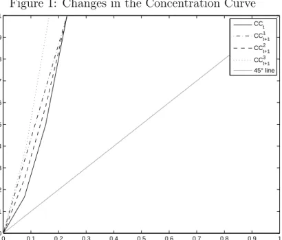
Figure 1: Changes in the Concentration Curve 0 0.1 0.2 0.3 0.4 0.5 0.6 0.7 0.8 0.9 1 0 0.1 0.2 0.3 0.4 0.5 0.6 0.7 0.8 0.9 1
Population share in ascending order of total income
Share of income of subgroup i
CC t CC1 t+1 CC2 t+1 CC3 t+1 45° line
Notes: This figure depicts Examples 1 to 3. In periodt the economy’s income vector is
y = (1 2 3 10 · · · 10)0 with number of individuals without loss of generality set equal to dim(y) = 13. The poorest three individuals belong to subgroupg, the remaining 10 indi-viduals belong to another subgroup. CCtplots the concentration curve of subgroup income
vectorxgin periodt. CCt+11 plots the concentration curve in periodt+ 1 as described in
Example 1,CC2
t+1as described in Example 2, andCCt+13 as described in Example 3. The
shift of the concentration curve to the left indicates a fall in the concentration coefficient.
jee and Podder (2007) establish a method which decomposes the change in the Gini into changes in the concentration coefficients, as well as changes in population and income shares of the different subgroups. Contrary to its counterpart decomposition by income sources from section 2.2, however, we show that the decomposition by population subgroups of Chatterjee and Podder (2007) is limited in its ability to provide insightful results. In par-ticular, we argue that this limitation is due to the inability to derive precise conclusions from changes in the concentration coefficients of the population subgroups. We will show this by means of three illustrative examples.
In the following, let us focus on a negative concentration coefficient of an arbitrary subgroup g, which decreases from one period to the next, i.e.
to follow Chatterjee and Podder (2007), who interpret such a change as “in-dicating that the within-group distribution shifted towards the lower-income population”(p. 282), suggesting “that the incomes of more [of group g] ... were concentrated in the lower half of the income distribution for the sample as a whole”(p. 282), or simply that “the distribution worsened”(p. 282) for subgroup g. Yet, the examples show that these interpretations of a negative change in the concentration coefficient may be misguided.
Consider an economy where the poorest three individuals belong to sub-group g receiving income of 1, 2 and 3 units, respectively. The rest of the population belongs to a different subgroup j 6=g and receives income of, say, 10 units each. Clearly, Cg <0.
Example 1. Imagine that from period t to t+ 1 income within subgroup g
is redistributed such that each of the three individuals now receives income of 2 units. It is apparent from Figure 1 that such a redistribution induces a fall in Cg. However, one can hardly interpret such a redistribution as a
worsening in the distribution of the income of subgroup g.
Example 2. Now imagine that each of the individuals of subgroupgreceives 2 additional units of income. Figure 1 illustrates that such a change leads to a decrease in the concentration coefficient. Yet again, this decrease in the concentration coefficient does not admit any of the interpretations offered by Chatterjee and Podder (2007).
Example 3. Imagine that the poorest individual dies between t and t+ 1. Subgroup g, thus, reduces in size to two individuals. Figure 1 shows that such a change in demography again leads to a decrease in the concentration coefficient of subgroup g. However, it would be mistaken to state that the incomes of more of subgroup g were concentrated in the lower half of the income distribution.
It is, of course, correct that a change that leads to more individuals of a subgroup being concentrated in the lower half of the income distribution, as
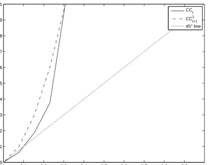
Figure 2: Change in the Concentration Curve due to a Fall in Income 0 0.1 0.2 0.3 0.4 0.5 0.6 0.7 0.8 0.9 1 0 0.1 0.2 0.3 0.4 0.5 0.6 0.7 0.8 0.9 1
Population share in ascending order of total income
Share of income of subgroup i
CC
t
CC1
t+1
45° line
Notes: In period t the economy’s income vector is y = (1 2 3 10 · · · 10)0 with number of individuals without loss of generality set equal to dim(y) = 13. The poorest four individuals belong to subgroupg, the remaining 9 individuals belong to another subgroup.
CCtplots the concentration curve of subgroup income vectorxgin periodt. CCt+1plots
the concentration curve in periodt+ 1 where the income of the 4th individual falls from 10 to 4 units. The shift of the concentration curve to the left indicates a fall in the concentration coefficient.
described by Chatterjee and Podder (2007), implies a decrease in the concen-tration coefficient. To see this, consider again the economy described above, but imagine that a fourth individual receiving an income of 10 units belongs to subgroupg. Since the rest of the population is larger than subgroupg and since each of the individuals not belonging to group g receives an income of 10 units, the median income is 10. Figure 2 shows that reducing the income of the fourth member of groupg from 10 to 4 units—which implies that more of the individuals in group g receive an income left of the median—reduces the concentration coefficient.
However, our illustrative examples made it abundantly clear that there are several other possible changes within the subgroup that can account for the same effect, which, however, are incompatible with the interpretation of
Chatterjee and Podder (2007). It is easy to think of many other, more com-plex, changes within a subgroup g, and even of changes in other subgroups
j 6=g, that can account for the same change in the concentration coefficient
Cg. It is thus difficult to relate changes in the Gini coefficient to underlying
changes in the population subgroups and, therefore, to derive policy relevant conclusions from the Gini trend decomposition of Chatterjee and Podder (2007). We want to stress, however, that the usefulness of the Gini elasticity referred to above is not affected by this result as it is obtained by increasing the income of the respective population subgroup proportionally such that the concentration coefficient does not change.
4
Conclusion
With this paper we intended to provide guidance for the use and interpreta-tion of Gini decomposiinterpreta-tions. We briefly reviewed the widely used, tradiinterpreta-tional decompositions of the Gini coefficient by income sources and population sub-groups originally formulated by, among others, Rao (1969) and Bhattacharya and Mahalanobis (1967), respectively. We then critically assessed more re-cent alternative decompositions and methodological enhancements.
We first showed that the approach of Podder (1993b), proposed to circum-vent the violation of the property of uniform additions of the traditional Gini decomposition by income sources, does not admit the interpretation intended by the author. We argued that marginal effects—in terms of the elasticity of the Gini coefficient with respect to the mean of an income source—should be used to examine the role of income sources for total income inequality as they provide unambiguously interpretable results.
Second, we pointed out that the traditional method of Fei et al. (1978) to decompose the change in the Gini coefficient into the underlying changes of the income sources becomes less tractable the more income sources are considered, and that the method suggested by Podder and Chatterjee (2002)
is at odds with the insights gained from marginal effects. We established a consistent method that allows quantifying the importance of income sources for the change in the Gini coefficient (for any number of income sources).
Finally, we examined in detail the Gini decomposition by population sub-groups put forth by Podder (1993a) and Chatterjee and Podder (2007) as an alternative to the traditional Gini decomposition. The method offers an intriguing way to circumvent the problem of the interaction term usually arising from the traditional Gini decomposition by population subgroups. We showed that the method, however, is unsuitable for tracing changes in the Gini back to underlying changes in the population subgroups as changes in the concentration coefficients do not allow for unambiguous conclusions.
Yet, we stressed that an analysis based on marginal effects in terms of the Gini elasticity is not affected by this shortcoming. The Gini elastic-ity still provides valuable insights regarding the sensitivelastic-ity of total income inequality with respect to changes in the income of population subgroups. We argued that, in this respect, the Gini decomposition by population sub-groups proposed by Podder (1993a) provides an analytical advantage over decompositions of other inequality indices. This advantage, which, to our understanding, has not been fully recognized by the income inequality liter-ature so far, may gain the approach of Podder (1993a) some new interest.
References
Achdut, L., 1996. Income Inequality, Income Composition and Macroeco-nomic Trends: Israel, 1979-93. EcoMacroeco-nomica 63 (250), S1–S27.
Bhattacharya, N., Mahalanobis, B., 1967. Regional Disparities in Household Consumption in India. Journal of the American Statistical Association 62 (317), 143–161.
Dis-tribution from Pre- to Post-reform New Zealand, 1984-1998*. Economic Record 83 (262), 275–286.
Cowell, F. A., 1988. Inequality decomposition: Three bad measures. Bulletin of Economic Research 40 (4), 309–312.
Cowell, F. A., 2000. Measurement of Inequality. In A. B. Atkinson and F. Bourguignon (Eds.), Handbook of Income Distribution, Chapter 2, 87–166, Amsterdam: North Holland.
Davis, B., Winters, P., Carletto, G., Covarrubias, K., Qui˜nones, E. J., Zezza, A., Stamoulis, K., Azzarri, C., DiGiuseppe, S., 2010. A cross-country com-parison of rural income generating activities. World Development 38 (1), 48–63.
Fei, J. C. H., Ranis, G., Kuo, S. W. Y., 1978. Growth and the family distribu-tion of income by factor components. The Quarterly Journal of Economics 92 (1), 17–53.
Fields, G. S., 1979. Income inequality in urban colombia: A decomposition analysis. Review of Income and Wealth 25 (3), 327–341.
Gini, C., 1912. Variabilit`a e mutabilit`a. C. Cuppini, Bologna.
Kimhi, A., 2011. Comment: On the Interpretation (and Misinterpretation) of Inequality Decompositions by Income Sources. World Development 39 (10), 1888–1890.
Lambert, P. J., Aronson, J. R., 1993. Inequality Decomposition Analysis and the Gini Coefficient Revisited. The Economic Journal 103 (420), 1221– 1227.
Lerman, R. I., Yitzhaki, S., 1985. Income Inequality Effects by Income Source: A New Approach and Applications to the United States. The Review of Economics and Statistics 67 (1), 151–156.
Mookherjee, D., Shorrocks, A., 1982. A Decomposition Analysis of the Trend in UK Income Inequality. The Economic Journal 92 (368), 886–902. Morduch, J., Sicular, T., 2002. Rethinking inequality decomposition, with
evidence from rural China. The Economic Journal 112 (476), 93–106. Paul, S., 2004. Income sources effects on inequality. Journal of Development
Economics 73 (1), 435–451.
Podder, N., 1993a. A New Decomposition of the Gini Coefficient among Groups and Its Interpretations with Applications to Australia. Sankhy¯a: The Indian Journal of Statistics, Series B (1960-2002) 55 (2), 262–271. Podder, N., 1993b. The disaggregation of the gini coefficient by factor
com-ponents and its applications to Australia. Review of Income and Wealth 39 (1), 51–61.
Podder, N., Chatterjee, S., 2002. Sharing the national cake in post reform New Zealand: income inequality trends in terms of income sources. Journal of Public Economics 86 (1), 1–27.
Pyatt, G., 1976. On the Interpretation and Disaggregation of Gini Coeffi-cients. The Economic Journal 86 (342), 243–255.
Pyatt, G., Chen, C., Fei, J., 1980. The Distribution of Income by Factor Components. The Quarterly Journal of Economics 95 (3), 451–473. Rao, V. M., 1969. Two Decompositions of Concentration Ratio. Journal of
the Royal Statistical Society. Series A (General) 132 (3), 418–425.
Shorrocks, A. F., 1982. Inequality Decomposition by Factor Components. Econometrica 50 (1), 193–211.
Shorrocks, A. F., 1984. Inequality decomposition by population subgroups. Econometrica 52 (6), 1369–1385.
Shorrocks, A. F., 1988. Aggregation issues in inequality measures. in Eich-horn, W. (ed.), Measurement in Economics Physica-Verlag, 429–451. Silber, J., 1989. Factor Components, Population Subgroups and the
Com-putation of the Gini Index of Inequality. The Review of Economics and Statistics 71 (1), 107–115.
Yitzhaki, S., Lerman, R. I., 1991. Income stratification and income inequality. Review of Income and Wealth 37 (3), 313–329.