Alma Mater Studiorum - Università di Bologna
DOTTORATO DI RICERCA IN METODOLOGIA STATISTICA PER LA RICERCA SCIENTIFICA
Ciclo XXVI
Settore Concorsuale di aerenza: 13/D1 Settore Scientico disciplinare: SECS-S/01
MULTIDIMENSIONAL ITEM RESPONSE THEORY
MODELS WITH GENERAL AND SPECIFIC
LATENT TRAITS FOR ORDINAL DATA
Presentata da:
Irene Martelli
Coordinatore Dottorato:
Chiar.mo Prof. Angela Montanari
Relatore:
Chiar.mo Prof. Stefania Mignani
To my family and Lorenzo, for their love and support.
i
Abstract
The aim of the thesis is to propose a Bayesian estimation through Markov chain Monte Carlo of multidimensional item response theory models for graded re-sponses with complex structures and correlated traits. In particular, this work focuses on the multiunidimensional and the additive underlying latent structures, considering that the rst one is widely used and represents a classical approach in multidimensional item response analysis, while the second one is able to reect the complexity of real interactions between items and respondents.
A simulation study is conducted to evaluate the parameter recovery for the proposed models under dierent conditions (sample size, test and subtest length, number of response categories, and correlation structure). The results show that the parameter recovery is particularly sensitive to the sample size, due to the model complexity and the high number of parameters to be estimated. For a suf-ciently large sample size the parameters of the multiunidimensional and additive graded response models are well reproduced. The results are also aected by the trade-o between the number of items constituting the test and the number of item categories.
An application of the proposed models on response data collected to investi-gate Romagna and San Marino residents' perceptions and attitudes towards the tourism industry is also presented.
iii
Acknowledgements
First and foremost I want to thank my supervisor Stefania Mignani for her con-stant attention, care and belief. Then, I would like to express my gratitude to Mariagiulia Matteucci for her precious and fundamental suggestions and supervi-sion during the preparation of the thesis. My work would not have been successful without her. Appreciation is extended to Cristina Bernini who has provided the data. My special thanks to my friends and colleagues Lucia and Violeta for their support during the whole period of the PhD.
v
Preface
Item response theory (IRT) falls within the wide context of the measurement of theoretical latent constructs, which are not observable by denition and can only be determined indirectly, through the use of other manifest variables.
IRT is extensively used in educational and psychological elds, where usu-ally a test consisting of a set of items is submitted to a sample of examinees to infer the individuals' unobservable characteristics (abilities). To this aim, IRT (Hambleton and Swaminathan, 1985; van der Linden and Hambleton, 1997) rep-resents the main methodological approach that allows to estimate both the item psychometric properties and the subjects' scores. Moreover, IRT shows a great potential in applications within behavioral sciences.
In the past, unidimensionality, i.e. the presence of a unique construct underly-ing the response process, was one of the most common assumption. Nevertheless, real data often suggest a multidimensional structure and, with the aim to infer such distinct latent traits, tests should include dierent subtests.
For this reason, models that allow the presence of more than one latent trait have been recently developed. The so called multidimensional IRT (MIRT) mod-els (see e.g., Reckase, 2009) are able to describe the complexity of the data, taking into account correlated abilities and also a possible hierarchical structure of la-tent traits. This is the reason why MIRT models perform better in tting the subtests if compared to separate unidimensional models.
Several approaches are possible within the multidimensional perspective: ex-plorative models, where all latent traits are allowed to aect all the item re-sponses, or conrmatory models, where all the relations between observed and latent variables need to be specied in advance. By using a conrmatory ap-proach, it is also possible to assume the simultaneous presence of general and specic latent traits underlying the response process (Sheng and Wikle, 2008). A further distinction can be made between non compensatory and compensatory models, where a lack in one trait naturally compensates for the other (Reckase, 2009).
In several applications, data are characterized by hierarchical structures and the introduction of dierent levels for latent dimensions permits to specify more
vi
general models. Specically, a proper hierarchy can be assumed to underlie the response process, where the highest level is associated with the overall trait, while dimensions representing more specic traits are located on lower level of the hierarchy.
High-order and additive models are two approaches that allow to include a general trait in addition to multiple specic traits. Particularly, in additive models, we can analyze the strength of the relationships between the specic latent traits and the associated test items directly as well as the strength of the relationships between the general latent trait and all the test items. This feature is particularly appealing for complex applications.
A nal distinction can be made according to the nature of the observable variables. Usually, in an educational testing framework we deal with binary items (i.e. correct/incorrect) while in psychological and behavioral researches items are typically ordinal, representing judgments or agreements. Dierent models for ordinal data have been developed according to the number of item parameters (e.g. partial credit models, graded response models) in a unidimensional context. On the contrary, within a multidimensional context, models for binary data are usually applied and, often, the available ordinal data are dichotomized, with a consequent loss of information. Models for ordinal data remain uncommon and were developed only for uncorrelated latent traits.
For these reasons, in this work we propose an extension of the unidimensional graded response model (Samejima, 1969) for ordinal data to multidimensional structures with correlated traits, namely the multiunidimensional and the ad-ditive structures. A further innovative and important aspect of our proposal deals with the estimation procedure, in fact, we propose a Markov chain Monte Carlo (MCMC) procedure for parameter estimation which we implement using the open-source software OpenBUGS.
Structure of the thesis
In the rst chapter some fundamental notions about IRT are introduced. A rst section illustrates the basic concepts and denitions characterizing the IRT ap-proach, with a brief description of unidimensional models for binary data. A
vii
second section focuses on unidimensional models for ordinal data and, in partic-ular, on the Samejima's model for graded responses. A nal section explains the reasons that have driven several developments of IRT towards its multidimen-sional generalization.
The second chapter introduces the MIRT approach. In the rst section the main features of these models are described, while in the second section a brief review on MIRT models for both binary and ordinal response is reported, together with a brief description of their most common estimation methods.
In the third chapter the main principles characterizing the Bayesian estimation in MIRT context are introduced. The rst section describes the general Bayesian framework, while the second section presents the available Bayesian estimation methods based on MCMC techniques. The third section briey introduces the functioning of OpenBUGS, which permits to easily run the most common MCMC algorithm, i.e. the Gibbs sampler.
In the fourth chapter two MIRT models for ordinal data with a complex structure are introduced in terms of specication, interpretation and estimation. The focus is on two MIRT models for graded responses and correlated latent traits: the multiunidimensional model, where items in each subtest characterize a single ability, and the additive model, where each item measures a general and a specic ability directly.
The fth chapter describes a simulation study that has been conducted in or-der to evaluate the parameter recovery of the estimation method for the proposed models. The simulation study design is illustrated in the rst section, while the second and the third sections report the results of the simulations performed for the multiunidimensional and the additive models for ordinal data, respectively.
In the sixth chapter an application of the proposed models to real data is presented. The application focuses on the investigation of residents' perceptions and attitudes towards the tourism industry.
In the seventh chapter conclusions and further research on applicative and methodological aspects are discussed.
Contents
1 An introduction to item response theory (IRT) 1
1.1 Basic concepts and denitions . . . 1
1.1.1 The concept of model in IRT . . . 2
1.1.2 IRT unidimensional models for binary data . . . 3
1.2 IRT unidimensional models for ordinal data . . . 5
1.2.1 Samejima's unidimensional graded response model . . . 7
1.2.2 Other unidimensional IRT models for graded responses . . . 9
1.3 Towards multidimensional models . . . 10
2 Multidimensional IRT (MIRT) models: a review 13 2.1 Main features of MIRT models . . . 13
2.1.1 Compensatory and noncompensatory approaches . . . 15
2.1.2 Conrmatory and exploratory approaches . . . 15
2.1.3 Underlying latent structures . . . 16
2.2 MIRT models for binary data . . . 19
2.3 MIRT models for ordinal data . . . 22
2.4 Estimation methods . . . 24
3 Bayesian estimation of MIRT models 27 3.1 Elements of Bayesian statistics in MIRT context . . . 27
3.1.1 Prior distribution choice . . . 28
3.1.2 Bayes' Theorem . . . 29
3.1.3 Marginal posterior distributions for model parameters . . . 30
3.2 Markov chain Monte Carlo methods . . . 31
3.2.1 Metropolis-Hastings algorithm . . . 35 ix
x CONTENTS
3.2.2 Gibbs sampler . . . 36
3.3 Bayesian computation using OpenBUGS . . . 38
4 MIRT graded response models with complex structures 41 4.1 MIRT graded response models (GRMs) . . . 41
4.1.1 Specication of the multiunidimensional GRM . . . 44
4.1.2 Specication of the additive GRM . . . 45
4.2 Person and item parameters: interpretation . . . 46
4.2.1 Ability parameters . . . 46
4.2.2 Multidimensional item discrimination . . . 46
4.3 Multiunidimensional GRM implementation . . . 47
4.3.1 Model specication . . . 48
4.3.2 Prior distributions . . . 48
4.3.3 Likelihood function for responses . . . 50
4.4 Additive GRM implementation . . . 51
4.4.1 Model specication . . . 51
4.4.2 Prior distributions . . . 52
4.4.3 Likelihood function for responses . . . 53
5 Simulation Study 55 5.1 Simulation study design . . . 56
5.1.1 Parameter recovery . . . 57
5.1.2 Estimated ability correlations . . . 57
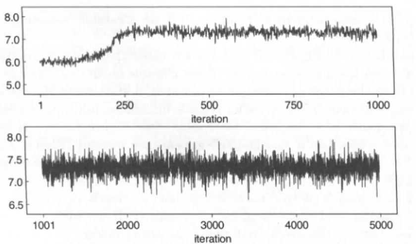
5.1.3 Convergence detection . . . 57
5.1.4 Bayesian t . . . 59
5.1.5 General simulation conditions . . . 60
5.2 Multiunidimensional GRM: simulations and results . . . 60
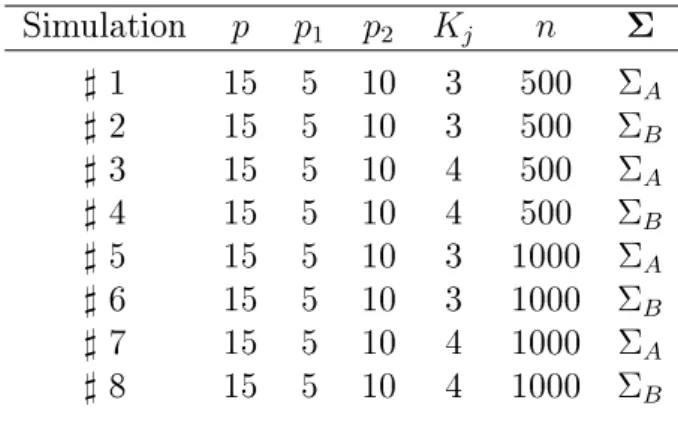
5.2.1 Simulation conditions . . . 60
5.2.2 Results . . . 61
5.3 Additive GRM: simulations and results . . . 64
5.3.1 Simulation conditions . . . 64
5.3.2 Results . . . 66
6 Application to real data: residents' attitudes towards tourism 75 6.1 Interpretation of model parameters . . . 75
CONTENTS xi
6.3 Results for the multiunidimensional GRM . . . 78 6.4 Results for the additive GRM . . . 82 6.5 Heterogeneity in resident perceptions . . . 86
7 Conclusions 89
Bibliography 92
Appendices 100
A OpenBUGS code for implemented models 101
A.1 OpenBUGS code: multiunidimensional and additive models for graded responses . . . 101
B R procedures for the simulation study 105
B.1 Multiunidimensional GRM: R code . . . 106 B.2 Additive GRM: R code . . . 109
List of Tables
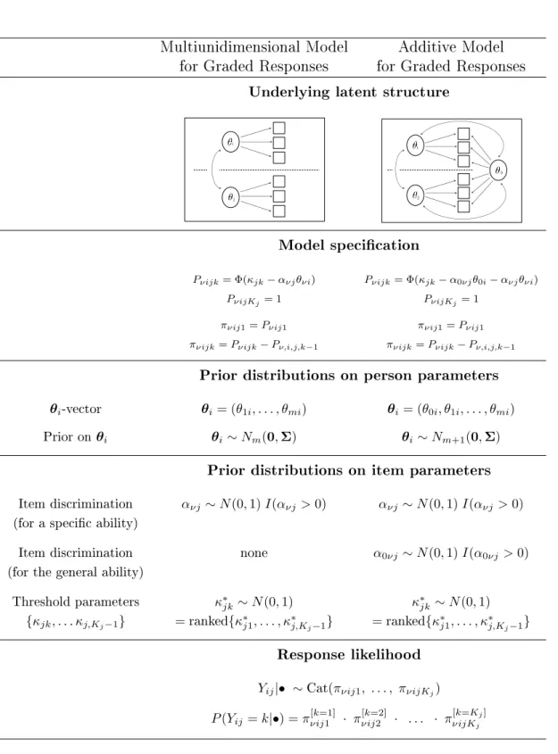
4.1 Main features of the proposed multiunidimensional and additive models for graded responses. . . 54 5.1 Simulation conditions for the multiunidimensional model for graded
responses. . . 61 5.2 Multiunidimensional model: block 1 simulation results for subtest
1 (median RMSEs and median absolute biases). . . 62 5.3 Multiunidimensional model: block 1 simulation results for subtest
2 (median RMSEs and median absolute biases). . . 62 5.4 Multiunidimensional model: real (r) and estimated (ˆr) ability
cor-relations. . . 63 5.5 Simulation conditions for the additive model for graded responses. 66 5.6 Additive model: block 1 simulation results for subtest 1 (median
RMSEs and median absolute biases). . . 68 5.7 Additive model: block 1 simulation results for subtest 2 (median
RMSEs and median absolute biases). . . 69 5.8 Additive model: block 2 simulation results for subtest 1 (median
RMSEs and median absolute biases). . . 70 5.9 Additive model: block 2 simulation results for subtest 2 (median
RMSEs and median absolute biases). . . 71 5.10 Additive model: real (r) and estimated (rˆ) ability correlations. . . 72 6.1 Prole of respondents. . . 77 6.2 Response frequencies for items about tourism benets (B1-B5) and
items about tourism costs (C1-C5). . . 78 6.3 Item parameter estimates for the multiunidimensional GRM. . . . 80
xiv LIST OF TABLES
6.4 Item parameter estimates for the additive GRM. . . 84 6.5 Normalized mean perception and attitude scores by age, gender,
List of Figures
1.1 Item characteristic curve for a binary item . . . 6
1.2 Item response functions for an item with ve categories . . . 6
1.3 Dichotomization of polytomous item responses, the dashed line indicates the observed category response. . . 8
2.1 Consecutive unidimensional latent structure. . . 16
2.2 Multiunidimensional latent structure. . . 17
2.3 Bi-factor latent structure. . . 17
2.4 Hierarchical latent structures. . . 18
2.5 Additive latent structure. . . 18
4.1 Dichotomization used for the MIRT graded response model speci-cation. The dashed line indicates the observed category response. 43 5.1 Bidimensional case for multiunidimensional and additive structures. 56 5.2 Examples of stationary chains. . . 58
6.1 Representation of the thresholds' parameter estimates for the mul-tiunidimensional model. . . 82
6.2 Representation of the thresholds' parameter estimates for the ad-ditive model. . . 85
Chapter 1
An introduction to item response
theory (IRT)
In this chapter we introduce the fundamental notions concerning item response theory (IRT). A brief description of IRT models for binary and ordinal data is carried out. Particular attention is given to the unidimensional Samejima's model for graded responses, which represents the starting point towards a generalization into a multidimensional context.
1.1 Basic concepts and denitions
IRT falls within the wide context of the measurement of theoretical latent con-structs. A latent construct is not observable by denition and it can only be determined indirectly, through the use of other manifest variables. Examples of latent constructs are the mathematics achievements of students, the satisfaction of a costumer about a product or service, the psychological status and all the situations that may refer to the concept of perception, e.g. depression and happi-ness. Another relevant eld of application of IRT methods is represented by the behavioral sciences, where the manifest variables, that are often ordinal, express a judge or an agreement to the phenomenon of interest.
If we consider the educational and psychological elds, where IRT is exten-sively used, we can say that IRT has the nal aim to measure abilities and atti-tudes of individuals through the responses on a number of test items. In other
2 1. An introduction to item response theory (IRT)
words, by using IRT models, we wish to determine the position of the individual along some latent dimensions, representing the unobservable characteristics of the individuals.
In IRT literature the latent traits are commonly called abilities, for the in-tensive use of IRT methods in the educational eld, where the constructs are represented by the students' latent abilities. The analysis of the relation between latent continuous variables and observed categorical variables is known in the statistical literature as latent trait analysis, that is the reason why in this thesis the words abilities, latent abilities and latent traits are all referred to the same concept.
The use of IRT as a measurement theory is fairly recent: in the pioneer work of Lord and Novick (1968) a rst formalization of the theory is expressed, on the basis of ideas and principles that raised in the thirties and forties. Improvements of IRT were due to the necessity to overtake the lacks of the classical test the-ory (CTT), for instance the sensitivity to sample conditions and the fact that in CTT individual abilities and test characteristics can be interpreted only in the same context (Hambleton et al., 1991). Moreover, IRT focuses on item rather than on individual score, while in the CTT the evaluation of test properties and item characteristics are not included. On the other side, IRT permits to evaluate individual ability and to describe the performances of the items on the test si-multaneously. For these reasons, IRT seemed to be an alternative and promising method to substitute CTT in theoretical and application elds, showing a wide and eective framework.
1.1.1 The concept of model in IRT
In IRT a model is dened by a mathematical function used to describe the con-ditional probability of a response given the latent ability, for an item with cat-egorical responses (Thissen and Steinberg, 1986). The mathematical function expresses how an examinee with a high position on a latent trait is likely to pro-vide a dierent response to an examinee with a low position on the trait (Ostini and Nering, 2006). The parametric model describes the relationship between the "observable", i.e. the examinee's performance in the test, and the "unobserv-able", the latent ability.
1.1 Basic concepts and denitions 3
In general, dierent models can be specied depending on:
• The structure of the data: binary or polytomous (nominal or ordinal)
re-sponses;
• The number of latent dimensions: unidimensional or multidimensional
mod-els;
• The distribution functions used to link responses and ability(ies); • The number of item parameters introduced in the model.
Concerning the rst point, IRT permits to specify dierent models depending on the kind of items we are dealing with, i.e. items with two response categories or items with more than two response categories (that, in turn, can be odered or not). The second point is a crucial choice in the model specication procedure: when only one ability aects the responses we are assuming unidimensionality, while when we need two or more latent traits to describe the correlation among the responses we are assuming multidimensionality. Moreover, the model depends on the probability distribution used to describe the relationship between the response and the examinee's ability(ies) and the number of parameters describing the item characteristics introduced. The most common probability models used are the normal distribution function (normal ogive models) and the logistic distribution function (logit models). Finally, a distinction can be made with reference to the number of item parameters, one, two or three, introduced in the model.
1.1.2 IRT unidimensional models for binary data
In order to illustrate the basic concepts and assumptions of IRT and to introduce the notation, we start from the simplest models: the unidimensional models for dichotomous responses (i.e. correct and incorrect). In this context there are three fundamental assumptions.
The rst assumption states that only one latent ability aects the item re-sponses (unidimensionality assumption).
The second assumption states that a change in the probability of a correct response, due to a change in the examinee latent ability, is completely described
4 1. An introduction to item response theory (IRT)
by the item characteristic curve (ICC). Thus, the ICC describes how the prob-ability of a response to an item changes relative to a change in the latent trait. As illustrated before, dierent distribution functions used to link responses and ability, i.e. dierent mathematical forms of the ICC, lead to dierent IRT mod-els. In any case the probability of a correct response is expressed as a function of person and item parameters.
The third assumption is the so called local independence assumption: re-sponses to a pair of items are statistically independent given the underlying la-tent ability. Local independence holds when the assumption of unidimensionality is true. Let consider a random vector of p item responses for the i-th
sub-ject (i = 1, . . . , n), denoted by Yi, and the corresponding observed responses,
yi = (yi1, . . . , yip). θi is the ability of the examinee i. The assumption of local
independence can be stated as:
P(yi|θi) = P(yi1|θi)P(yi2|θi). . . P(yip|θi) = p
Y
j=1
P(yij|θi).
When local independence holds, there is one latent variable underlying the responses and, conditionally to this latent variable, responses are assumed to be independent.
The unidimensional IRT model for binary data expresses the probability πij
of a correct response by the subject ito the item j as a function of the predictor ηij, which depends on θi and onξj, the vector of parameters characterizing item
j, forj = 1, . . . , p:
ηij =f(θi,ξj). (1.1)
The so called probit or normal ogive model is obtained when a normal distribution is used (1.2), whereas when we use the logistic distribution we get the logit model (1.3)1:
1Normal ogive models and logistic models have dierent ICCs for equivalent set of item
parameters values. It can be proved (Haley, 1952; Birnbaum, 1968) that the two formulations are equivalent in terms of predicted probability through the introduction of a scaling constant 1.702 into the logistic model, in order to balance for dierences in ICCs. When this constant is introduced in the model, the predicted probabilities dier by less than 0.01 for each level of ability (Haley, 1952): |Φ(ηij)−exp(1.702ηij)/[1 +exp(1.702ηij)]|<0.01.
1.2 IRT unidimensional models for ordinal data 5 πij = Φ(ηij)⇒Φ−1(πij) =ηj (1.2) πij = exp (ηij) 1 +exp(ηij) ⇒logit(πij) =ηij , (1.3)
whereΦis the standard normal cumulative distribution function. Dierent unidi-mensional models can then be obtained by introducing a dierent number of item parametersξj describing the item characteristics. The simplest case has only one
item parameter ξj = {βj}, and βj is called diculty parameter. An example of
one-parameter logistic model is the Rasch model (Rasch, 1960) and if we con-sider a logarithmic transformations of the scale of person and item parameters (Fischer, 1995), the predictor becomes ηij =θi−βj.
If ξj = {αj, βj} a discrimination parameter αj is added to the model and
we are in the case of two-parameter models. The predictor (1.1) becomes ηij =
αjθi −βj: model (1.2) becomes the two-parameter normal ogive model (Lord,
1952) while model (1.3) becomes the two-parameter logistic model (Birnbaum, 1968).
A further extension can nally be done by introducing a guessing parameter
γj for each item, leading to three-parameter models whereξj ={αj, βjγj}(Lord,
1980). See Reckase (2009) for an exhaustive description of such models.
With respect to the ICC, the parameters αj, βj and γj represent the slope,
the location and the lower asymptote, respectively.
1.2 IRT unidimensional models for ordinal data
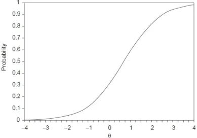
Models briey presented above are all referred to dichotomous responses, never-theless items with multiple response options exist and their use is quite common in behavioral sciences. IRT models for polytomous items operate in a dierent way from binary models. In the latter case the knowledge of the characteristics of a response determines also the characteristics of the other complementary re-sponse, while for polytomous items this feature does not hold anymore and each category function must be modeled separately (Samejima, 1996). In Figure 1.1 the ICC for a binary item is reported, while Figure 1.2 shows dierent response
6 1. An introduction to item response theory (IRT)
functions for an item with ve categories.
Figure 1.1. Item characteristic curve for a binary item
Figure 1.2. Item response functions for an item with ve categories From Figure 1.2 we can see how, for ordered items, the category response functions are not all monotonic: only the curves related to the rst and the last categories are, respectively, monotonically decreasing and increasing. The presence of non-monotonic functions raises some complications: these functions cannot be described only in terms of discrimination and diculty parameter, as in the binary case. The choice of the proper mathematical form and the estimation
1.2 IRT unidimensional models for ordinal data 7
of parameters for such unimodal functions is a relevant issue. For ordered polyto-mous items this problem has been solved by treating polytopolyto-mous items basically as `concatenated dichotomous' items (Samejima, 1969, 1996): dichotomizations of item response data are combined in order to get suitable response functions for each item category.
As we will illustrate more in detail later, several models for ordinal data exist as result of extensions of the models for binary data. The simplest model for ordinal items is the partial credit model (Masters, 1982), which is an extension of the Rash model for binary items, i.e. with one item parameter. Despite its wide use, it focuses on the scoring of the individuals and its restrictive assumptions make it inadequate for modeling purposes, especially in complex contests. In this work we focus on the Samejima's graded response model, which is the general-ization of the two-parameter IRT model for binary data. This choice has been lead by the consideration that models that include also the guessing parameter, even if they are appropriate educational eld, do not suit well in the context of behavioral science, where individuals typically express opinions.
1.2.1 Samejima's unidimensional graded response model
The graded response model for ordinal data was developed by Samejima in 1969. Examples of graded responses are Lykert-type scales (strongly-disagree, dis-agree, neutral, dis-agree, and strongly agree) and responses ordered on the basis of a range of scores.Let consider a set of p ordinal items, Y1, . . . , Yj, . . . , Yp, where each item has
Kj categories, indexed by k. In the parametrization of the model we consider
that the lowest score on itemj is1, while the highest score isKj and each item is
characterized byKj−1thresholds or boundariesκj1, . . . , κj,Kj−1. The probability
of achieving k or higher categories is assumed to increase monotonically with
a growth in the latent ability (Samejima, 1996; Reckase, 2009), therefore the thresholds must satisfy the so called order constraint: κj1 <· · ·< κj,Kj−1.
Concerning the dichotomization procedure mentioned above, Samejima's (1969) graded model is based on the probability that an item response will be observed in category k or higher: the probability πijk that the i-th subject will select
8 1. An introduction to item response theory (IRT)
lower boundary for the category (κk−1) minus the probability of answering above
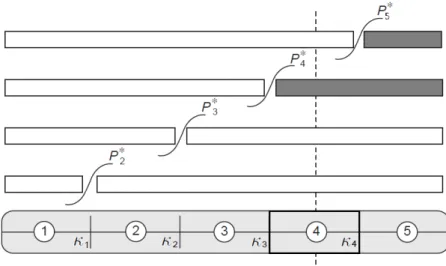
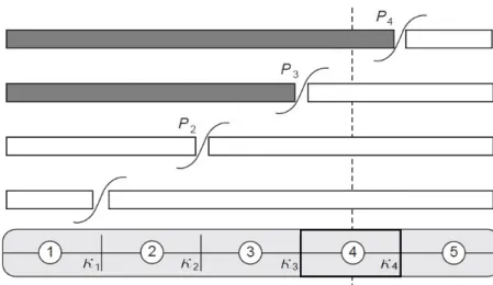
the category's upper boundary (κk). Figure 1.32 describes the dichotomization
method used in Samejima's models, a dashed line is used to represent an hypo-thetical response in category k = 4: the probability to have a response in such category can be computed as Pi∗4−Pi∗5, where in general withPik∗ =P(Yij ≥k|θi)
we denote the probability of accomplishing step k at a given level of θ.
Figure 1.3. Dichotomization of polytomous item responses, the dashed line indicates the observed category response.
The probability that thei-th examinee's response will fall in thek-th category
on item j can thus be written as:
πijk=P(Yij =k|θi) = Pik∗ −P
∗
i,k+1 , (1.4)
where Pi∗1 and Pi,K∗ j+1 are assumed to be respectively 1 and 0, in order to ensure
that the probability of each category can be determined from (1.4). The two-parameter normal ogive and logistic formulations of the model can be obtained from (1.4). The normal ogive form of the Samejima's model for graded responses
1.2 IRT unidimensional models for ordinal data 9 is given by: πijk=P(Yij =k|θi, κjk, κj,k+1) = 1 √ 2π αjθi−κjk Z αjθi−κj,k+1 e−t2/2dt . (1.5)
From expression (1.5), we can observe that the discrimination parameter αj,
i.e. the slope of the response functions, is constant between all dierent category responses of a given item. This constraint ensure to avoid negative probabilities (Steinberg and Thissen, 1995). The boundary parameters κjk vary within an
item, according to the order constraint κj,k−1 < κjk < κj,k+1, and at each level
of θ = κjk, the examinee has a probability of 0.5 of endorsing the category
(Reeve, 2002). Pik∗ is the trace line reecting the probability that an examinee's
response will fall in that scoring category or a higher, at any specic level of latent ability θ. The graded model response function P(Yij = k|θi) reects the
rate of examinees responding to thek-th category through the dierent levels of θ, that is a non-monotonic curve, with the exception of the curves associated to
the extreme categories, as previously pointed out in Figure 1.2 (Thissen et al., 2001).
1.2.2 Other unidimensional IRT models for graded
responses
Several models for items with two or more ordered responses have been developed. An assortment of these models, together with their features, has been introduced by van der Linden and Hambleton (1997) and van der Ark (2001). In addition to Samejima's graded response model (1969), other widely applied IRT models for ordinal data are the partial credit model (Masters, 1982) and its extension, the generalized partial credit model (Muraki, 1992). The partial credit model is an extension to the case of ordinal items of the Rash model for binary items, i.e. with one item parameter. On the other side, the Samejima's graded response model is the generalization of the two-parameter IRT model for binary data.
In partial credit model and in its generalization, the category responses on the item represent the levels of performance (Reckase, 2009). As well as in
10 1. An introduction to item response theory (IRT)
the graded response model, we have thresholds between adjacent scores: an ex-aminee's performance is on the left or the right side of a threshold with a spe-cic probability. Here the dichotomization procedure involves only two category boundaries for a given item, see Ostini and Nering (2006) for a detailed discussion about dierences between Samejima and Rasch dichotomization approaches.
Mathematical expressions for the partial credit model and the generalized partial credit model are presented in (1.6) and (1.7), where D = 1.702 is the scaling constant: πijk =P(Yij =k|θi) = exp{Pk u=1(θi−κju)} PKj v=1exp{ Pk u=1(θi−κju)} (1.6) πijk =P(Yij =k|θi) = exp{Pk u=1Dαj(θi−βj+κju)} PKj v=1exp{ Pk u=1Dαj(θi−βj+κju)} . (1.7)
In the generalized partial credit model the assumption of constant discrimi-nation parameter of test items is relaxed, in fact αj parameters may vary across
items. Reckase (2009) provides an exhaustive illustration of such models. Other IRT models for polytomous items have been proposed by Bock (1972), Andrich (1978, 1982), Thissen and Steinberg (1984), and Rost (1988). All these models refer to an unidimensional underlying ability structure.
1.3 Towards multidimensional models
Unidimensional models are suitable when tests are made to measure only one latent ability (Sheng and Wikle, 2009). There are some advantages in the use of such unidimensional models: i) they have quite simple mathematical forms; ii) they perform well in tting the data in several empirical applications; and iii) they are rather robust to violations of assumptions (Reckase, 2009).
Nevertheless, real interactions between examinees and test items are not sim-ple as described in unidimensional models. A person is likely to use more than a single ability in the response process, on one hand, and the problems posed in a test can require several abilities in order to get the right solution, on the other
1.3 Towards multidimensional models 11
side.
Multidimensional IRT (MIRT) models were developed to have a more accurate description of interactions between persons and test items. In particular, in MIRT models a vector of latent abilities is introduced, instead of assuming a single person parameter.
In other words, MIRT models deal with quite common circumstances where an examinee requires multiple abilities in order to respond to an item. In this case, more than one latent construct is measured by that item. One of the most famous example in the educational eld is a mathematical test item presented as story that requires both mathematical and verbal abilities to arrive at a correct score (Fox, 2010), where both mathematical and reading comprehension skills are involved in the answering process.
Chapter 2
Multidimensional IRT (MIRT)
models: a review
As previously pointed out, the latent space that has to be measured may be more complex than the one underlying unidimensional IRT models. The so called MIRT models are used when separate latent abilities are encompassed in the observed responses for an item.
In this chapter we introduce the MIRT approach. In particular, we show how dierent models can be specied depending on the latent ability structure hypothesized to underlie the response process. A literature review on MIRT models for both binary and ordinal data is reported. A nal section describes the most common estimation methods in IRT and MIRT frameworks.
2.1 Main features of MIRT models
The assessment of dimensionality is a key topic in IRT and in the latent variable framework. A review of methods for an empirical detection of the structure of tests with binary items was made by Tate (2003). In his work, a particular atten-tion is given to the assessment of the test statistical structure as subtended from the relations between examinees and items. This aspect should be an important
14 2. Multidimensional IRT (MIRT) models: a review
part of the development, evaluation, and maintenance of large-scale test.
Several IRT models are based on a common postulate: the assumption of unidimensionality. However, the local independence assumption holds only if the latent space is entirely specied. For this reason, many eorts for the characteri-zation of the concept of dimensionality and for its detection have been made. We can say that an accurate and unequivocal denition of dimensionality does not exist yet. This is due to the fact that the phenomenon is latent by nature, hence a direct comparison with observed results is not possible.
Hambleton and Swaminathan (1985) justied the unidimensionality assump-tion with the presence of a dominant trait able to explain the examinees' re-sponses. In this sense, we can imagine that a single trait always exists but crucial points are if the dominant trait is suciently strong and in which way it dominates the others. Conversely, Traub (1983) argued that unidimensionality is probably more the exception than the rule, with respect to the skills necessary to answer to the items on most cognitive tests.
Some weak features of the unidimensionality assumption have been reviewed by Adams et al. (1997), with the aim to propose a MIRT model. The use of unidimensional models might be improper for tests intentionally built from sub-components that are assumed to measure dierent abilities. IRT models seem to be robust to these violations of unidimensionality, especially with highly cor-related latent constructs. In fact, if we assume the existence of a single latent ability, it can be seen as the dominant factor reecting the dierent composition of the items. On the other hand, when a test is made by mutually exclusive sub-tests of items or when the underlying dimensions are not highly correlated, the use of a unidimensional model can bias the parameter estimation, adaptive item selection and trait estimation. The problem is highlighted especially in adaptive testing, when the examinees are administrated dierent combinations of items and the traits underlying the performance may reect the dierent composition of the items (Matteucci, 2007).
Finally, as shortly described at the end of Chapter 1, the assessment of knowl-edge, competencies and achievement is going more and more towards a multidi-mensional evaluation. The reason of the widely use of MIRT models in recent studied is that the actual interactions between examinees and test items are com-plex and necessitate to be framed in a multidimensional background. A clarifying example reported in Matteucci (2007) concerns the assessment of prociency in
2.1 Main features of MIRT models 15
the University context, where the student's evaluation is typically multidimen-sional at each level: within a single course and during all the University career, students are evaluated on the basis of multiple competencies.
2.1.1 Compensatory and noncompensatory approaches
MIRT models can be classied in two main groups: compensatory and non-compensatory models, depending on the way the vector of latent abilities, θ,is combined with item parameters to obtain the probability of responses to the item.
In compensatory models we use a linear combination of the values of θ in the
specication of the response probabilities, by using a logistic or a normal ogive form. This approach implies that dierent combinations of elements in θ can
yield the same sum, and the direct consequence is a compensation eect: if a
θ-value is low, but another one is appropriately high, the sum can be the same.
In noncompensatory models, dierent latent abilities used to solve an item are separated and each part is used as an unidimensional model. Then the global probability is obtained as the product of the probabilities of each unidimensional part. Nonlinearity raises in relation to the use of the product of such probabilities, and the compensation property does not hold (Reckase, 2009).
2.1.2 Conrmatory and exploratory approaches
Another classication of MIRT models can be done with reference to the available information at the model specication step. Mainly, the investigation of multidi-mensionality can be conducted by using two dierent approaches: the exploratory and the conrmatory approaches.
In the exploratory approach no prior knowledge is included in the model, in terms of relationship between items and latent traits.
When the number of latent abilities is specied in advance, the method is not merely explorative and we are in a conrmatory context. In line with the conrmatory approach, not only the number of latent variables is pre-specied but also their relationships with the items. In fact, the researcher can use prior knowledge to dene which items load on which factors.
16 2. Multidimensional IRT (MIRT) models: a review
2.1.3 Underlying latent structures
In this paragraph a brief review of dierent multidimensional latent structures is reported. For simplicity, gures are referred to the simplest case of a test consisting of two subtests. Circles represent latent traits and squares represent observed item responses. Subtests are indicated with dashed lines.
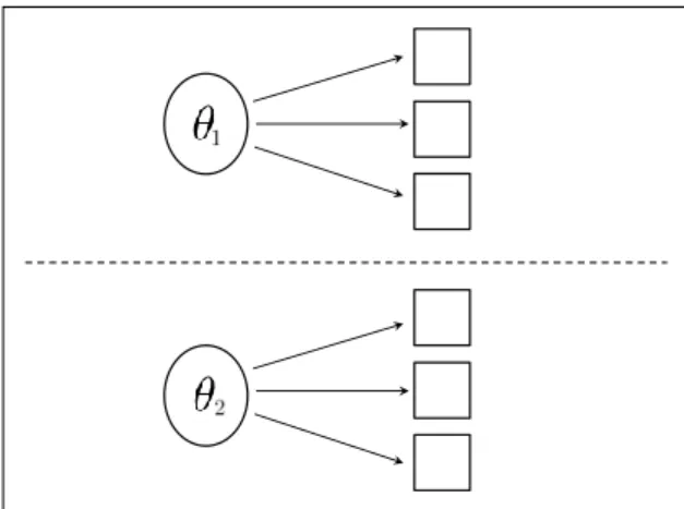
Consecutive unidimensional model In Figure 2.1 is illustrated the so called consecutive unidimensional approach, where simple unidimensional IRT models are tted to each subtest in a sequential way. Fitting this model, we obtain person measures for every specic ability, but a direct estimation for the relation between them is not feasible (Huang et al., 2013).
Figure 2.1. Consecutive unidimensional latent structure.
Multiunidimensional model Figure 2.2 reports the underlying structure for the between-item MIRT model (Wang et al., 2004), also called multiunidimen-sional approach (Sheng and Wikle, 2007), where abilities are allowed to correlate and the intensity of such associations can be obtained directly.
Bi-factor model The well known bi-factor model, rst introduced by Holzinger and Swineford (1937), where a general (or common) ability, θ0, and a specic
ability are assumed to aect the response to each item, is illustrated in Figure 2.3. This is a case where there is within-item multidimensionality, i.e. single
2.1 Main features of MIRT models 17
Figure 2.2. Multiunidimensional latent structure.
items measure more than one latent trait. This approach ignores the association between latent abilities.
Figure 2.3. Bi-factor latent structure.
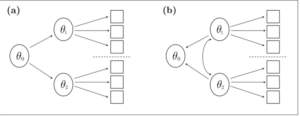
Hierarchical models Figure 2.4 shows the latent structure assumed for MIRT hierarchical models, where the hierarchical structure in general and specic la-tent constructs is modeled explicitly: items in the same subtest measure a specic ability and, in turn, each specic ability is inuenced by a general ability. Dif-ferent hierarchical models can be specied depending on the relation between specic and overall abilities: if each specic ability is a linear function of the overall ability we are in the case illustrated in (a), while if each specic ability
18 2. Multidimensional IRT (MIRT) models: a review
linearly combines to form the overall ability we are in the case showed by (b) (Schmid and Leiman, 1957; Sheng and Wikle, 2008).
Figure 2.4. Hierarchical latent structures.
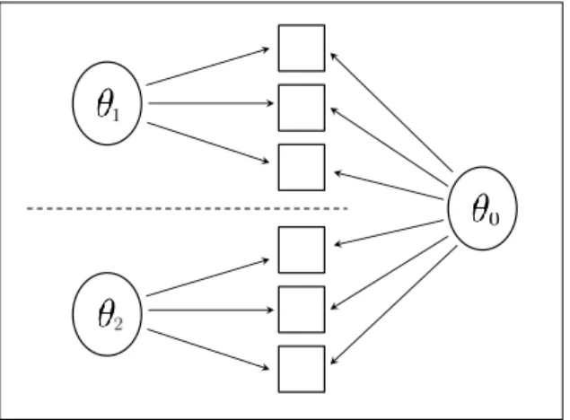
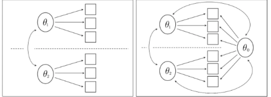
Additive model In the additive model presented in Figure 2.5 the latent struc-ture is such that the response to a test item is aected both by the general and the specic latent traits, so that the latent abilities form an additive structure (Sheng and Wikle, 2009). This model has a latent structure similar to the bi-factor model, but here all the latent constructs are allowed to correlate.
2.2 MIRT models for binary data 19
2.2 MIRT models for binary data
MIRT is a methodology that has been developed with the principal aim of dealing with the situation of complexity in psychological measurement when several latent abilities inuence the individual's performance on a given item (Reckase, 1997). By introducing a person trait and item discrimination parameters for each ability measured by a test item, MIRT models permit separate inferences with reference to each distinct latent dimension of an examinee (Ackerman, 1993).
Two parameter normal ogive model for binary data
Let consider a test consists of p multiple choice items, each measuring m latent
abilities, θ1i, . . . , θmi. Let Y = [Yij]n×p represents the data matrix, i.e. a matrix
containing nexaminees' responses topbinary items, so that, fori= 1, . . . , nand j = 1, . . . , p, Yij is dened as:
Yij =
1, if examineei answers item j correctly
0, if examineei answers item j incorrectly.
Reckase (1985) derived a multidimensional extension of the compensatory unidi-mensional two-parameter model, that in its normal ogive formulation becomes:
P(Yij = 1|θi,αj, βj) = Φ m X ν=1 ανjθνi−βj ! = = √1 2π Pm ν=1ανjθνi−βj Z −∞ e−t2/2dt . (2.1)
Each individual is characterized by a vector θi = (θ1i, . . . , θmi)of latent
abili-ties, where m is the number of latent dimensions measured by a generic item, in
contrast to the unidimensional case, where they are classied by only one latent ability θi.
20 2. Multidimensional IRT (MIRT) models: a review
multiple dimensions: αj = (α1j, . . . , αmj) , where j represents the item number
and m shows the dimension to which the discrimination value is related. If the
discrimination parameter related to dimension ν, ανj , is high, it means that
such dimension has a great inuence in determining an examinee's success on item j. Finally, βj is a scalar parameter determining the location in the latent
space where the item provides maximum information.
Multiunidimensional model for binary data
As illustrated in the work of Sheng and Wikle (2007), the elements in the vector of discrimination parameters αj = (α1j, . . . , αmj) can be considered as factor
loadings in factor analysis. If a rotation is performed so that each item loads on one factor only, the vector of discrimination parameters can be simplied toαj =
(0, . . . ,0, ανj,0, . . . ,0), and we can get the expression for the multiunidimensional
model for binary data, where each latent trait is related to a single set of items, from (2.1). The underlying latent structure of such model is illustrated in Figure 2.2. Let consider a test consisting of p items. The test is structured into m
subtests, each one composed by pν items that measure one latent trait. The
probability that the individualiwill obtain a correct response to itemjbelonging
to the ν-th subtest is given by:
P(Yνij = 1|θνi, ανj, βj) = Φ (ανjθνi−βj) =
1 √ 2π ανjθνi−βj Z −∞ e−t2/2dt ,
where ανj is a scalar parameter reecting the item discrimination, θνi is a scalar
parameter reecting the individual's ν-th ability, and βj is a scalar parameter
representing the location in the latent space where the item provides maximum information.
Additive model for binary data
The additive MIRT model for dichotomous data proposed by Sheng and Wikle (2009) assumes an underlying latent structure such that both specic abilities and an overall ability aect directly the individual response to a test item, resulting
2.2 MIRT models for binary data 21
in an additive structure (see Figure 2.5).
If we consider again a test containing p items structured into m subtests
(each one composed by pν items), according to the additive MIRT model for
binary data, the probability that the individual i will obtain a correct response
to itemj belonging to the ν-th subtest is given by:
P(Yνij = 1|θ0i, θνi, α0νj, ανj, βj) = = Φ(α0νjθ0i+ανjθνi −βj) = α0νjθ0i+ανjθνi−βj Z −∞ 1 √ 2πe −t2/2 dt , (2.2)
where θνi is a scalar parameter representing the examinee's ability in the ν-th
dimension, θ0i is the i-th individual parameter related to the overall ability,α0νj
is thej-th item discrimination parameter with reference to the overall abilityθ0i,
ανj is the item discrimination parameter with reference to the specic abilityθνi,
and βj is a scalar parameter representing the location in the latent space where
the item provides maximum information.
The expression in (2.2) implies that the probability that an individual endorses an item is directly inuenced by two latent traits: a general ability and a specic one (Sheng and Wikle, 2009).
A more detailed description of the models for binary data presented above goes beyond the purpose of this study. Our decision to focus the analysis on the additive structure has been driven by the fact that this latent structure, according to which both the specic and general latent traits directly underlie all the test items, represents a plausible and fairly detailed approximation of the real interactions between individuals and item responses. On the other hand, the multiunidimensional model is simpler than the additive, but it is regularly used in MIRT applications.
The exposition of these two models has been done in order to furnish a more complete background on the latent structures that we will discuss in detail for the case of ordered responses.
22 2. Multidimensional IRT (MIRT) models: a review
2.3 MIRT models for ordinal data
A multidimensional formalization of IRT models for graded responses has been developed as an extension of the unidimensional version by several authors. In this section we present some works that focus on multidimensional models for ordered items. These works have not necessary developed in an IRT context, but also in the framework of conrmatory factor analysis. Basically, the interest in adopting such models raised to face the widespread use of Likert items (Likert, 1932), and in general other ordered scales, on questionnaires in sociological and psychological measurement. The extensive availability of such data has led, in the last two decades, to the need of new progressions towards a multidimensional version of IRT model for graded responses.
We begin by introducing some notation. As in the case for dichotomous items, let consider a test made by p multiple choice items, each measuring m
latent traits, θ1, . . . , θm. Now the data are collected in a matrix, Y = [Yij]n×p,
containing n examinees' responses to p ordered items, thus, for i= 1, . . . , n and j = 1, . . . , p, Yij is dened as: Yij =
1, if the answer of examinee i to itemj falls in category1 2, if the answer of examinee i to itemj falls in category2 ... ...
Kj, if the answer of examinee i to itemj falls in categoryKj
where 1 and Kj are the lowest and the highest score for item j, respectively.
Muraki and Carlson (1995) developed a MIRT model for polytomously scored items on the basis of Samejima's graded response model in the full information factor analysis context. In their work, they show how the factor analytic model for categorical variables is based on the assumption that the response process, say Zij, is an underlying not observable variable and, for each subjecti, realized
into the vector of observed ordered item responses Yi = (Yi1, Yi2, . . . , Yip). They
2.3 MIRT models for ordinal data 23
latent traits, θ1i, θ2i, . . . , θmi, and the factor loadings αj1, αj2. . . , αjm. Thus:
Zij =αj1θ1i+αj2θ2i+· · ·+αjmθmi+εij =α0jθi+εij ,
where εij is an unobserved random variable that is assumed to be distributed
as N 0, σ2
j
. Muraki and Carlson (1995) introduced the threshold parameter
γjk associated with the k-th category of item j, and modeled the unobservable
response process according to the psychological mechanism, that is Yij = k if
γj,k−1 ≤Zij < γjk, for k = 1, . . . , Kj, γj0 =−∞, and γjKj = +∞. The
probabil-ity to get the response category k of item j by examinee i, given the examinee's m-dimensional latent trait and assuming a normal ogive model, is formalized as:
P(Yij =k|θi) = 1 (2π)12σj γjk Z γj,k−1 exp ( −1 2 Z ij −α0jθi σj 2) dZ . (2.3)
Model (2.3) can be rewritten in a more familiar way with item response models, by applying some transformation of the variables (see Muraki and Carlson (1995) for the detailed procedure). The authors focus on uncorrelated latent dimensions (bi-factor latent structure) and furnish a detailed procedure of the Expectation Maximization (EM) algorithm in a marginal maximum likelihood estimation con-text (the matter of estimation methods will be covered in the next section). The proposed algorithm has been implemented in the POLYFACT computer pro-gram (Muraki, 1993), which calculates the factor loadings via the principal factor method adopted to the product-moment correlation matrix. The program treats the observed responses as continuous variables (Muraki and Carlson, 1995).
In the study by Ferrando (1999) a comparison between three dierent item response models for graded responses has been made, focusing on a continuous response model based on linear factor analysis, a censored response model, where the graded responses are considered to be censored continuous variables, and a multidimensional graded response model in the formulation given by Muraki and Carlson (1995). They observed that, even though there have been several appli-cations of the unidimensional graded response model to attitude and personality data, applications of the multidimensional version of the model are not common.
24 2. Multidimensional IRT (MIRT) models: a review
Ferrando (1999) concludes showing that the solutions were similar for the three models considered, but that the estimation method could aect the results.
A more recent work by Edwards (2010a) falls within the context of conrma-tory item factor analysis models. He developed a relatively user friendly package, MultiNorm (Edwards, 2010b), where the user can t multidimensional graded (or dichotomous) response models characterized by a multiunidimensional or a bi-factor underlying latent structure. The estimation technique used in this work belong to the Markov chain Monte Carlo (MCMC) techinques. Again, for a further discussion on estimation methods see the next section.
Other applications of MIRT models for graded responses, with empirical ex-amples regarding mainly the eld of educational assessment and the psychological reactance, can be found in Yao and Schwarz (2006), Fu et al. (2010), Brown et al. (2011) and van der Ark et al. (2011). It is worth to remark that the latent struc-tures assumed in these studies were prevalently the multiunidimensional structure (Figure 2.2) and the bi-factor structure (Figure 2.3).
Considering this scarcity of existing research about MIRT models for ordinal outcomes, especially for complex cases, in this work we take into consideration the one represented by an additive underlying latent structure (Figure 2.5), after having introduced the multiunidimensional case (Figure 2.2).
2.4 Estimation methods
In IRT models, as well as in MIRT models, the characteristics of interest are the person's abilities and the item parameters: dierent values of these parameters lead to dierent response probability. Nevertheless, these two important char-acteristics are both unknown and the available data are represented only by a collection of responses given by a sample of examinees.
Concerning the estimation procedure, we need to consider two relevant fea-tures: the rst one is that the response model is not linear and the second one is that is not possible to observe the latent trait θ. It implies that the estimation
is similar to perform a nonlinear regression with unknown predictor values. Starting from the available data, the focal objective is in the determination of theθvalues for every individual and the item parameters from the item responses.
2.4 Estimation methods 25
context of the maximum likelihood (ML) or in a Bayesian framework.
The estimation procedure is in general aected by the way the probabilities of the responses are theorized. There are two main interpretations of proba-bility: one of them is the stochastic subject interpretation, where the observed examinees are considered as xed and probabilities reect the unpredictability of specic events. Here the latent variables are constructed as unknown xed pa-rameters. The other interpretation of probability is the random sampling, where the examinees are considered as a representative random sample from a popula-tion, so that it raises the needing to specify a specic distribution of the latent trait and the latent variables are constructed as random.
In the framework of ML estimation, three main methods can be identied:
• The joint maximum likelihood (JML);
• The conditional maximum likelihood (CML); • The marginal maximum likelihood (MML).
In the JML and CML methods we are in the context of the stochastic subjects interpretation of probability, i.e. xed latent variables, whereas in the MML method we are in the random sampling interpretation framework and the latent variables are treated as random.
The applicability of JML and CML is pretty limited. The JML method works by simultaneously estimating item and person parameter through an iterative procedure. This method is quite simple but the complexity of the algorithm increases with the number of observations. The standard limit theorems do not apply and the resulting parameter estimators are not consistent (Andersen, 1970). The CML was a method suggested by Andersen (1970) and based on the avail-ability of a sucient statistic for the avail-ability in order to simplify the maximum likelihood conditioning on it. There is a relevant problem which limits the appli-cability of such method: most models, including the quite simple unidimensional two parameter model, do not have simple sucient statistics (Johnson, 2007).
The MML estimation method is the most widely applied and, by considering the joint probability of a certain response pattern given the latent trait and integrating out of the individual likelihoods, it denes the marginal probability
26 2. Multidimensional IRT (MIRT) models: a review
of observing the item response pattern. To obtain the parameters estimates, the EM algorithm is used (Ayala, 2009).
A single estimated latent trait value can be associated to each individual through maximum a posteriori or expected a posteriori techniques. In general, all the ML estimation methods consider xed item parameters. Conversely, in the Bayesian context, both the latent abilities and the item parameters are regarded as random variables.
As we will see later more in detail in the next chapter, the adoption of a fully Bayesian approach implies several advantages. It allows a joint estimation of item parameters and individual abilities and it permits to include uncertainties about item parameters and abilities, and in general prior beliefs, in the prior distributions. MCMC estimation of IRT and MIRT models can be then viewed as an alternative to MML estimation, where the approximation of multiple integrals involved in the likelihood function, especially for increasingly complex models, may represent a serious problem.
Chapter 3
Bayesian estimation of MIRT
models
This chapter introduces the main ideas and functioning characterizing the Bayesian approach for estimation purposes, with a particular focus on the simulation-based methods for parameter estimation. Available Bayesian estimation methods based on MCMC techniques for MIRT models are also presented.
3.1 Elements of Bayesian statistics in MIRT
con-text
According to the Bayesian approach, all the model parameters, i.e. person and item parameters in our case, are random variables, each one with its prior distri-bution reecting the prior information available and the uncertainty about their real values before the observation of the data.
All the MIRT models so far illustrated (for both binary and ordinal items) are specied with the nal aim to express the data-generating process as a function of the unknown person and item parameters. These are likelihood models and present the density of the data conditional on the model parameters. In order to
28 3. Bayesian estimation of MIRT models
formulate a Bayesian model, we need to specify:
• A prior distribution for each unknown model parameter; • A likelihood model reecting the data-generating process.
Once the data are observed, the prior information is updated with the in-formation contained in the observed data and a posterior distribution is made, which permits to perform direct inference about parameters.
3.1.1 Prior distribution choice
A key point in Bayesian framework is the possibility to specify prior distributions for the unknown model parameters with the aim to exploit background informa-tion and beliefs available before the collecinforma-tion of the sample. All these context information are expressed as probability distributions and, as a result, are re-ected in a prior distribution. On the other hand, the conditional probability distribution is specied to reect the observed data.
One of the main objection to the Bayesian framework regards the specica-tion of these prior distribuspecica-tions, that can be considered extensively subjective and arbitrary (Gelman, 2008). It has to be noticed that the choice of the prior distributions, made at the moment of model specication, is subjective by de-nition.
Therefore, only prior distributions expressing prior ideas can be considered correct in this setting and, even if the choice is subjective, it cannot be considered arbitrary since it reects the researcher's thought (Fox, 2010). In addition, it is possible to specify the so called vague priors, that are objective non informative prior distributions indicating ignorance around the unknown parameter values.
The branch of objective Bayesian statistics rely on the specication of objec-tive prior distributions. Even though it does not need any subjecobjec-tive contribution, we have to consider that a specic point of strength of Bayesian methodology is the possibility of including beliefs and prior information in model specication, and objective Bayesian methods do not allow to do that.
The inclusion of prior beliefs can increase the reliability of the statistical inference. In IRT and MIRT frameworks, item responses represent the observed data and we can include other sources of information in the model through the
3.1 Elements of Bayesian statistics in MIRT context 29
a priori model. These are circumstances where data-based information is slight, and where prior information can signicantly improve the statistical inference (Fox, 2010).
3.1.2 Bayes' Theorem
Let consider a set of N observations, denoted by y = (y1, . . . , yN), that are the
numerical realization of the random vectorY = (Y1, . . . , YN), which follows some
probability distribution. Let denote with p(y) the probability density (mass) function of the continuous (discrete) variable Y.
Now let assume that, starting from the observed responses, we are inter-ested in measuring the unknown person (θ) and item (ξ) parameters, denoted
by λ = (θ,ξ). We denote with p(λ) the prior distribution reecting the beliefs on unknown parameters. The termp(y|λ)reects the information about λfrom
the vector of observed values y. In general, we can be interested in the sampling
distribution and the likelihood function if we consider it as a function of the data or as a function of the parameters, respectively. Usually, the distribution of the parameters given the data is of main interest. According to the Bayes' Theorem, the conditional distribution of λgiven the response data is
p(λ|y) = p(y|λ)p(λ)
p(y) ∝ p(y|λ)p(λ), (3.1) where ∝ denotes proportionality. The term p(λ|y) is the posterior density of the parameter λ given both prior and sample information and, for continuous
quantities,p(y) =Rλ∈Λp(y|λ)p(λ)dλ(whereΛdenotes the set of all the possible
values of λ).
Since we are interested in person and item parameters, we replace expression (3.1) with
p(θ,ξ|y) = p(y|θ,ξ)p(θ)p(ξ)
p(y) ∝ p(y|θ,ξ)p(θ)p(ξ), (3.2) wherep(θ)is the prior for person parameters θ, p(ξ)is the prior for item param-eters ξ and these prior densities are assumed to be independent from each other,
30 3. Bayesian estimation of MIRT models
thus p(θ,ξ) =p(θ)p(ξ).
The denominator of expression (3.2) is called the data marginal density, marginal likelihood, or integrated likelihood. Its evaluation can be a time costly process, so that, when the knowledge of the shape of the posterior p(θ,ξ|y) is enough for the study purposes, we can focus on the unnormalized density func-tion: p(y|θ,ξ)p(θ)p(ξ)(Fox, 2010).
The statement of the well-known Bayes' Theorem (Bayes and Price, 1763) is represented by the expression reported in (3.2). In particular, the expression
p(θ,ξ|y) ∝ p(y|θ,ξ) p(θ) p(ξ) is a factorization representing the product of the likelihoodL(y;θ,ξ)and the prior density, as typicallyL(y;θ,ξ) =p(y|θ,ξ). All the sample information regarding person and item parameters is contained in this likelihood function.
A relevant distribution for the inference process is the so called joint posterior density p(y,θ,ξ). This density can be factorized as follow:
p(y,θ,ξ) = p(θ,ξ|y)p(y) (3.3) = p(y|θ,ξ)p(θ)p(ξ). (3.4)
From the expressions above we can observe that the joint posterior distribution can be factorized in two dierent ways: (i) as the marginal density of the data and the posterior of the unknown parameters (3.3), and (ii) as the prior distributions of the parameters and the likelihood of (θ,ξ) giveny (3.4).
3.1.3 Marginal posterior distributions for model
parame-ters
In order to make inference, the joint posterior distribution reported in (3.2) is used. Since this high-dimensional distribution has a complex form, and conse-quently it usually shows an analytically intractable expression, we need to focus on one of the unknown parameters, and consider the other as a nuisance param-eter.
More precisely, if we are interested in the distribution ofθ, we assume ξ as a
3.2 Markov chain Monte Carlo methods 31
we obtain the marginal posterior density for person parameters:
p(θ|y) = Z ξ∈Ξ p(θ,ξ|y)dξ = Z ξ∈Ξ p(y|θ,ξ)p(θ)p(ξ) p(y) dξ ∝ Z ξ∈Ξ p(y|θ,ξ)p(θ)p(ξ)dξ. (3.5)
When we are interested in the distribution of ξ, we consider θ as a nuisance
parameter and thus we integrate out all the values of θ, getting the marginal
posterior density for item parameters:
p(ξ|y) = Z θ∈Θ p(θ,ξ|y)dθ = Z θ∈Θ p(y|θ,ξ)p(θ)p(ξ) p(y) dθ ∝ Z θ∈Θ p(y|θ,ξ)p(θ)p(ξ)dθ. (3.6)
In general, the information contained in the joint and/or marginal poste-rior distributions are summarized by the posteposte-rior mean (median) and standard deviation. Concerning the joint posterior distribution of person and item pa-rameters, as previously pointed out, several diculties arise as a result of its high-dimensionality and analytical intractability. Nonetheless, with reference to the marginal posterior densities of person (3.5) and item (3.6) parameters, the same diculties remain, as the mathematical expressions are not always known. These computational problems can be solved by the use of simulation based techniques. In particular, the MCMC method is a very useful technique that we will be briey describe in the next section.
3.2 Markov chain Monte Carlo methods
The Bayesian approach based on MCMC techniques has increased its popularity in the estimation of unidimensional and multidimensional item response models. A twofold motivation can drive the use of such method. First of all, it can
32 3. Bayesian estimation of MIRT models
represent an eective substitute to the classical EM algorithm implemented in the MML estimation. In fact, it works with simulation and introduces an informative prior distribution in the estimation process and, unlike the MML method, the Bayesian approach considers both the person parameters and item parameters as random variables. Secondly, it can also be seen as a compensatory instrument to the EM algorithm. The posterior distribution generated through the MCMC techniques can be used to evaluate the suitability of the normal approximations in the MML, so that we can compare the two approaches with reference to the accuracy of parameter recovery.
As we will see in this section, MCMC is a very useful and relatively straight-forward method to make inference when we have to face with a very complex model, where it is actually dicult to sample or directly simulate from the pos-terior distribution. This represents a common situation in a MIRT context.
In particular, the Gibbs sampler is a widely used MCMC algorithm consisting in a quite precise scheme to create suitable samples from the posterior density. Moreover, this method is not very constraining and fairly simple to implement, if compared with other methods. For the motivations mentioned above, MCMC strategies have been implemented in IRT background by several researchers and many studies have been made in order to investigate the properties of these methods. Of particular interest is also the evaluation of model parameter recovery in comparison with the classical methods.
If we perform a comparison between the MCMC technique and the classical MML estimation, we can summarize the main advantages of the MCMC approach in:
• the exibility regarding the modeling of all the connections between latent
and observed variables;
• the appropriateness for more complex models;
• the non-sensitivity to the choice of starting values (unlike the EM
algo-rithm).
Two relevant works that perform Bayesian estimation using the Gibbs sampler in an IRT context are the works of Albert (1992) and Béguin and Glas (2001). In the rst one, the Gibbs sampler for the unidimensional two parameter model for binary data is implemented, and the MCMC algorithm is compared with the