Title
Air Pollutant Dispersion
Author(s)
Lei, S; Hou, Y; Wang, X; Liu, K
Citation
IEEE Transactions on Industrial Informatics, 2017, v. 13 n. 3, p.
995-1005
Issued Date
2017
URL
http://hdl.handle.net/10722/237017
Rights
IEEE Transactions on Industrial Informatics. Copyright © IEEE.;
©2016 IEEE. Personal use of this material is permitted.
Permission from IEEE must be obtained for all other uses, in any
current or future media, including reprinting/republishing this
material for advertising or promotional purposes, creating new
collective works, for resale or redistribution to servers or lists,
or reuse of any copyrighted component of this work in other
works.; This work is licensed under a Creative Commons
Attribution-NonCommercial-NoDerivatives 4.0 International
License.
Abstract--Air pollution problems are attracting increasing attention, especially among developing countries with frequent haze events. Renewable energy sources such as wind power are expected to help relieve such environmental concerns. However, air pollution issues under such a changing energy structure receive inadequate attention. Mostly, constraints for total pollutant emissions are considered in unit commitment (UC) and economic dispatch (ED) problems. In this paper, we propose a UC model with wind power that considers the dispersion of air pollutants. The dispersion process is described by models involving meteorological conditions and the system’s geographical distribution, to estimate the spatial distribution of air pollutants, i.e. the concentration of ground-level air pollutants at monitored locations such as load centers. A penalty cost is introduced based on this estimation. Particulate matter 2.5 micrometers or less in diameter, the major air pollutant concerning most developing countries, is selected as the focus of this work. To properly estimate and sufficiently utilize the benefits of wind power for air pollutant dispersion control, robust optimization is applied to accommodate wind power uncertainty. Case studies justify this consideration of air pollutant dispersion, and demonstrate the effectiveness of the proposed model for improving load centers’ air pollution control and utilizing wind power benefits.
Index Terms--Air pollutant dispersion, Gaussian plume model, robust optimization, unit commitment, wind power.
NOMENCLATURE
A. Indices:
i Index of thermal units, i=1, … , NG w Index of wind farms, w=1, … , NW j Index of loads, j=1, … , ND
l Index of transmission lines, l=1, … , NL t Index of time intervals, t=1, … , T
This work was supported in part by National Natural Science Foundation of China under Grant 51677160, the Theme-based Research Scheme through Project No. T23-701/14-N, the Research Grant Council of Hong Kong SAR under Grants ECS739713 and GRF17202714, Basic Research Program-Shenzhen Fund (JCYJ20150629151046877), and research funding from State Grid Corporation of China (SGLNSY00FZJS1601337).
S. Lei and Y. Hou are with the Department of Electrical and Electronic Engineering, The University of Hong Kong, Hong Kong; Y. Hou is also with The University of Hong Kong Shenzhen Institute of Research and Innovation, Shenzhen, China (email: [email protected], [email protected]).
X. Wang is with the School of Chemistry and Environment, South China Normal University, Guangzhou, China (email: [email protected]).
K. Liu is with the China Southern Power Grid CO., Ltd., Guangzhou, China (email: [email protected]).
Copyright © 2016 IEEE. Personal use of this material is permitted. However, permission to use this material for any other purposes must be obtained from the IEEE by sending a request to [email protected].
B. Parameters:
sui /sdi Start-up/shut-down cost of thermal unit i λi /γi /βi Fuel cost coefficients of thermal unit i mui /mdi Minimum up/down-time of thermal unit i fil Power flow distribution factor (PFDF) of
transmission line l due to thermal unit i
fwl PFDF of transmission line l due to wind farm w fjl PFDF of transmission line l due to load j Fl Power flow limit of transmission line l
Pimax/Pimin Upper/lower limit for real power output of thermal
unit i
URi /DRi Ramp-up/down rate limit of thermal unit i Pjt Power demand of load j at time t
wt
P Forecastedmeanpoweroutputof wind farm w at time t
ˆ
wt
P Deviation from forecast of wind farm w at time t C. Variables:
Oit Binary on/off decision of thermal unit i at time t SUit Binary start-up decision of thermal unit i at time t SDit Binaryshut-down decision of thermal unit i at time t
b it
P Real power dispatch decision of thermal unit i at time t in the base case
u it
P Adaptive real power dispatch decision of thermal unit i at time t considering wind power uncertainty
Pwt Uncertain power output of wind farm w at time t
I. INTRODUCTION
ANY developing countries have witnessed frequent haze events in recent years. In China, for example, smog covered the major eastern cities of the country for over a week in winter 2013. More recently, severe haze hit Beijing in early December 2015, causing disruption for schools and companies, cancelled flights, and other issues. This kind of event has drawn worldwide attention to air pollution problems, as particulate matter 2.5 micrometers or less in diameter (PM2.5), the major cause of haze, is extremely harmful to human health due to its capability to deeply penetrate into human lungs and the blood stream. According to reports by the United Nations Environment Programme [1] and the World Health Organization (WHO) [2], air pollution is one of the world’s worst environmental health risks, causing millions of premature deaths and trillions of US dollars in economic cost.
As a major consumer of fossil fuels, the electric system is responsible for a high proportion of air pollutants emissions, with coal-fired plants the major source of PM2.5 and secondary
Unit Commitment Incorporating Spatial
Distribution Control of Air Pollutant Dispersion
Shunbo Lei,
Student Member, IEEE
, Yunhe Hou,
Senior Member, IEEE
, Xi Wang, and Kai Liu
PM2.5 formation elements SO2 and NOX. Dominant portion of power is supplied by coal in U.S., Germany, Australia, England, China, etc. Researchers and practitioners in power systems are accountable for the urgent need for better air pollution control. In some pioneering research works, the total amount of emitted pollutants was considered, typically formulated as a quadratic function of the real power output of thermal units. Constraints or penalty costs were introduced based on this summation of pollutants emissions [3]-[6]. In [7], the operation of various flue gas desulfurization systems was also accounted for. However, one essential aim of emission regulations is to limit ground-level air pollutant concentration (GLAPC), especially at “monitored locations” such as load centers with a high population density—places where there is more concern or interest about air quality. Following U.S. government efforts in the 1960s and 1970s such as the Clean Air Act of 1970, considerable research has been devoted to studying the dispersion of emitted air pollutants, i.e., to consider the resulting GLAPC at monitored locations [8]-[10]. Environmental science models describing the dispersion process of pollutants emitted from thermal units have been introduced to estimate GLAPC. This estimation, as an index, has been included as constraints or as a penalty cost in optimization problems of power system operations.
Nevertheless, industry practice for emissions regulations in power systems is still normally based on total emission limits, rather than consideration of GLAPC. Also, the past several decades has seen only a limited number of papers published by power system researchers that study GLAPC issues. There are likely two reasons for this modest level of effort. First, as air pollutant dispersion is an extremely complex process involving atmospheric movement, chemical reactions, etc., obtaining an estimation with acceptable accuracy is not easy. Plus the fact that electric systems are just one of many sources of air pollutants such as traffic, wildfires, etc., thermal units’ responsibilities are difficult to identify quantitatively, which is the second major reason. However, as we now have a much clearer understanding of the severe human health risks due to air pollution, these relevant topics deserve much more attention. As such, many mature and reliable dispersion models are now available. Governments are also much more willing to spend money in air pollution control. With the development of detection, computation and communication technologies for the emerging smart grid [11], air pollution control based on GLAPC information is important and can be practical for existing power systems.
Additionally, enormous renewable energy sources, especially wind power, has been integrated into power systems all over the world [12]. Besides relieving a potential energy crisis, wind power is also expected to reduce environmental pollution. One straightforward yet critical topic is to study the benefits of wind power integration in terms of CO2 and air pollutants emissions reduction. To the best of the authors’ knowledge, all recent papers are based on the amounts of emissions such as in [13]-[18], while the essential relief in terms of GLAPC has not been analyzed. Specifically, in [13]-[16] wind power benefits in terms
of carbon emission control were studied. On the other hand, in [17], a study based on the Ireland system indicates that wind power could be ineffective in SO2 and NOX emission reduction. A dispatch model minimizing NOX emission is proposed for systems with stochastic wind power in [18].
In summary, recent studies of wind’s environmental benefits has concentrated on the total amount of carbon or other air pollutants emitted, while other essential benefits of wind power, such as GLAPC reduction, were not analyzed. As mentioned above, it is well recognized that it is critically important to look into the dispersion of air pollutants emitted by thermal units [8]-[10], [19]. Without consideration of air pollutant dispersion, wind power’s benefits in terms of air pollution control can be greatly undermined.
As one of the most important power system operation problems, unit commitment (UC) models minimize cost by optimizing each power plant’ on/off states and power dispatch [20]. Based on the above arguments, this work proposes a UC model that considers wind power benefits in terms of dispersion control of air pollutants. A dispersion model that considers meteorological conditions and the system’s geographical distribution is applied to describe the dispersion of air pollutants emitted by thermal units. Thus, GLAPC at monitored locations (load centers in this paper) is estimated and rendered a cost. That is, the spatial distribution of air pollutants are considered. The cost can be in the form of penalty costs, taxes for thermal units, or subsidies for influenced customers in load centers, etc. As wind power is uncertain in nature, robust optimization is employed to ensure robust feasibility of commitment decisions [21]-[24]. Thus, the system can be relieved from harsh spinning reserve requirements to accommodate wind power uncertainty and to prevent even worse emissions results. That is, robust optimization is applied to appropriately accommodate wind power uncertainties in terms of spinning reserve scheduling, so that the benefits of wind power for air pollutant dispersion control can be properly estimated and sufficiently utilized. A modified IEEE 14-bus system and the real-world Guangdong Grid system are used to demonstrate the effectiveness of the proposed UC model and analyze how wind power can help control air pollutant dispersion. The main contributions of this paper are summarized as follows:
1)A novel UC model is proposed and studied, in which the dispersion of air pollutants emitted by thermal units is considered. A review of major dispersion models is also presented. Meteorological conditions and the system’s geographical distribution are included in the applied plume model, to achieve better air pollution control in load centers, namely the spatial distribution control of air pollutant dispersion. Note that our method of air pollutant dispersion consideration can be easily extended for applications in problems such as economic dispatch (ED) and generation expansion planning.
2)Wind power benefits in air pollution control are studied. The reasons and methods to explicitly consider this issue are presented. Robust optimization is employed to handle wind power uncertainty to avoid its benefits being undermined by harsh spinning reserve requirements. The proposed model better
utilizes wind power benefits on this issue. The analysis focuses on PM2.5, which currently receives inadequate attention by power system researchers, with the aim of these results to provide advice and information for system operators and policy-makers.
The remaining parts of this paper are organized as follows. In Section II, air pollutant dispersion models are presented and discussed. In Section III, the proposed UC model is formulated. Section IV introduces the solution algorithm for the formulated problem. Case studies are included in Section V for illustration. Section VI concludes this paper.
II. AIR POLLUTANT DISPERSION MODELS
Toestimateathermal unit’scontributiontotheGLAPCofa specificmonitoredlocation,a model describing the dispersion of pollutants is necessary. First, the emission rate functions of thermal units for different kinds of pollutants are briefly summarized.
TheNOX emission rate function is highly non-linear in P (real power output). While most researchers generally apply a function with both polynomial and exponential terms, some use a second order polynomial function instead. For SOX and particulate matter, including the focus of this work PM2.5, emission rates are normally seen as proportional to coal consumption, i.e., generally quadratic to P. Thus, the PM2.5 emission rate of unit i at time t can be described as:
2
( b) b
it i it i it i
E c P b P a (1) where ai, bi, and ci denote emission coefficients.
Air pollutants are transported by atmospheric movements, i.e. dispersed, when emitted by thermal units at the above rate. From simple fixed-box models to the much more sophisticated plume and puff models, many different dispersion models have been developed to describe the dispersion process and predict the resulting GLAPC. For point sources including thermal units, both plume and puff models are extensively employed. As sketched in Fig. 1, a plume model describes air pollutants as a plume emitted from a stack, while a puff model regards thermal units as sources of a series of continuously overlapping puffs. Both models may assume some types of distribution for the dispersion in the cross-wind direction (y) and the vertical direction (z).
In the literature, some studies have used the plume model for its maturity, while others have used the puff model as it is more flexible for considering the non-steady state of meteorological conditions. To assert that one model is superior to the other is unreasonable and unnecessary. As mentioned, air pollutant dispersion is an extremely complex process related to complicated atmospheric movements, chemical reactions, meteorological conditions, etc. In environment science, it is believed that the critical point is to select a suitable and applicable model for the specific application. In this paper, based on literature ([4], [8]-[10], and [25]-[29]), a relatively comprehensive comparison of these two types of popularly used models is summarized and presented in Table I. Note that the practical application of these models normally demands efforts
x y z Win d di rect ion Δh x y z Win d di rect ion (a) (b) H
Fig. 1. Schematics for two major dispersion models: (a) Plume model; (b) Puff model.
TABLEI
COMPARISON OF PLUME AND PUFF MODELS
Plume model Puff model
State assumption Straight-line, steady-state Non-steady state
Model features Fits seen & experience More abstract modeling
Applicable range Limited to 50km Long range (200-300km)
Pollutant sources Point/line/area sources Point/line/area sources
Applicable pollutant types Particulate matter, NOX, SO2, CO Particulate matters, NOX, SO2, CO Emission
description Continuous release
Quasi-instantaneous, short-term release
Dispersion coefficients setup
Relatively more available & mature references
Limited available references
Data
requirements Need less data
Need more detailed data (spatial/temporal effects)
Time step/scale
Release time much greater than transition time from source to receptor
Release/sampling time very short compared to transition time
Preferable applications
When simple output required, maximum concentration considered Complex terrain scenarios (coastal effects, etc.) Major shortcomings
Naturally not for varying meteorological conditions
Difficulty in coefficients setup, overlook in-puff fluctuations
* EPA-
recommended scenarios
Near-field Long-range, complex wind-field
*EPA-approved
model developments
AERMOD, ISC3, BLP,
OCD, etc. CALPUFF, etc.
* EPA: U.S. Environmental Protection Agency
such as model adjustments, parameters tuning, grid cell modelling, etc.
In this paper, the Gaussian plume model, which is the most widely used model for describing the dispersion of continuous-release plumes, is applied for the following reasons:
1)Thermal units are point sources with a continuous release of pollutants. Their emissions can be better described by a contaminated plume. The release time is also greater than the transition time of the plume.
2)The plume model considers emissions as a plume starting from the stack of each thermal unit, while the puff model considers emissions as puffs independent of their source. Thus, it
is much more straightforwardto usetheplumemodeltodescribe the effect of thermal units on the air pollution of monitored locations.
3)This work considers a predicted GLAPC on load centers in a day-ahead UC problem. A model with simple inputs and simple outputs is preferred and desired for possible practice, since the much more detailed data necessary for the puff model can be inaccurate or unavailable.
Based on the applied plume model, as sketched by Fig. 1(a), a thermal unit’s contribution at time tr to the GLAPC of a load center, which is the monitored locations in this study, can be summarized as: r 2 2 2 2 2 2 2 1 exp 2 2 y it ijt y z x y x z x d E H C w I I d I d I d (2)
where w represents wind speed, dx and dy are the downwind
direction and cross-wind direction distances between load j and thermal unit i, Iy and Iz are emission constants determined by
many factors such as geographical/meteorological conditions and air pollutant dissipation situations, and H is the effective stack height of the thermal units. Interested readers may refer to [25] for more details. In this work, the aforementioned parameters are all assumed known. Equation (2) actually estimates the spatial distribution of air pollutants quite conservatively. Such a conservative estimation in turn leads to decisions that are sufficiently effective in terms of air pollutant dispersion control for the future day. Note that the time indices of Cijtr and Eit are different due to the transition time of the
emitted pollutants from a thermal unit to a load center. In this work we consider our study in a geographical area where the longest transition time is about one hour [10]. In addition, the polluting coal units normally supply the base load and do not significantly change their power output in each hour. More importantly, the responsibility of each thermal unit towards GLAPC at load centers is given a linear cost in this paper. Thus, it is not necessary to explicitly model this transition time into our UC formulation. For simplicity and clarity, denote Kij as the “air
pollutants dispersion coefficient” between generation i and load j
under specific meteorological conditions, which means we can re-write (2) and apply (1) to get:
r
2
[ ( b) b ]
ijt ij it ij i it i it i
C K E K c P b P a (3) Equation (3) reveals a roughly quadratic relationship under specific conditions. Note that if thermal unit i is on the downwind side of load center j, Kij should be zero. Although a
basic plume model is based on a steady-state assumption, it can actually be modified to handle scenarios with varying meteorological conditions, complex terrain, and other special cases such as calm winds, stagnation conditions, and variable wind direction. Wind speed is one of the major factors influencing the air pollutant dispersion process. It is worth mentioning that as shown in [10], one day can be approximately split into two halves, i.e. day and night, to have two different wind scenarios, each with a different relatively stable wind speed and wind direction. This conforms to the steady-state assumption of the plume model and justifies its application here. In this
paper, average wind speeds and directions for day and night are used. To consider more spatially or temporally varying meteorological conditions, the plume model can be adjusted for better performance, and the puff model may be more applicable in some cases. Techniques or models such as grid cell partitioning [30] or the RNG k-ε turbulence model [31], may also be necessary.
III. PROBLEM FORMULATION
In this section, a novel UC model with wind power that considers air pollutant dispersion is formulated, with the aim of ensuring the benefits that wind power provides for the spatial distribution control of air pollutants. The first part presents and explains the objective function. The second part describes the constraints, including a robust feasibility check.
A. Objective Function
A deterministic form of the objective function is adopted here to avoid over-conservativeness of the worst-case cost of robust optimization. The objective function (4) consists of three parts: 1) the commitment costs (CC) corresponding to start-up and shut-down operations of thermal units; 2) the base-case dispatch cost (BDC) under the nominal scenario with forecasted mean wind power outputs; and 3) the air pollutant dispersion cost (APDC) with the “price” αj.
min(CCBDC)APDC 1 1 ( ) G N T i it i it t i CC su SU sd SD
2 1 1 [ ( ) ] G N T b b i it i it i it t i BDC P P O
2 1 1 1 [ ( ) ] G D N N T b b j ij i it i it i it t j i APDC K c P b P a O
(4)Thus, the objective function considers both the common UC cost (UCC, including CC and BDC) and the proposed APDC introduced below.
As for the APDC, this cost actually exists even though industry practice does not normally have a tax or charge in this form. For example, reference [32] estimates the cost resulting from environmental damage caused by NOX, SO2 and PM10, including human health impacts. However, to completely determine the real economic cost of human health harm and environmental pollution resulting from the dispersion of emitted air pollutants is far too difficult, and would involve issues such as policy-making, pollution remediation, public health, etc. Thus, APDC is introduced as a penalty cost in this paper instead. This cost is different from the UCC as it is not really an existing charge. Instead, the APDC is mathematically included to drive changes in UC decisions and costs. However, we do incorporate some practical considerations, including population density and background pollution, when setting this penalty cost. This approach means that the APDC has correlated relationships with damage costs due to the impact of air pollutants on the environment and human health, and with pollution treatment costs typically shouldered by the government.
TABLEII
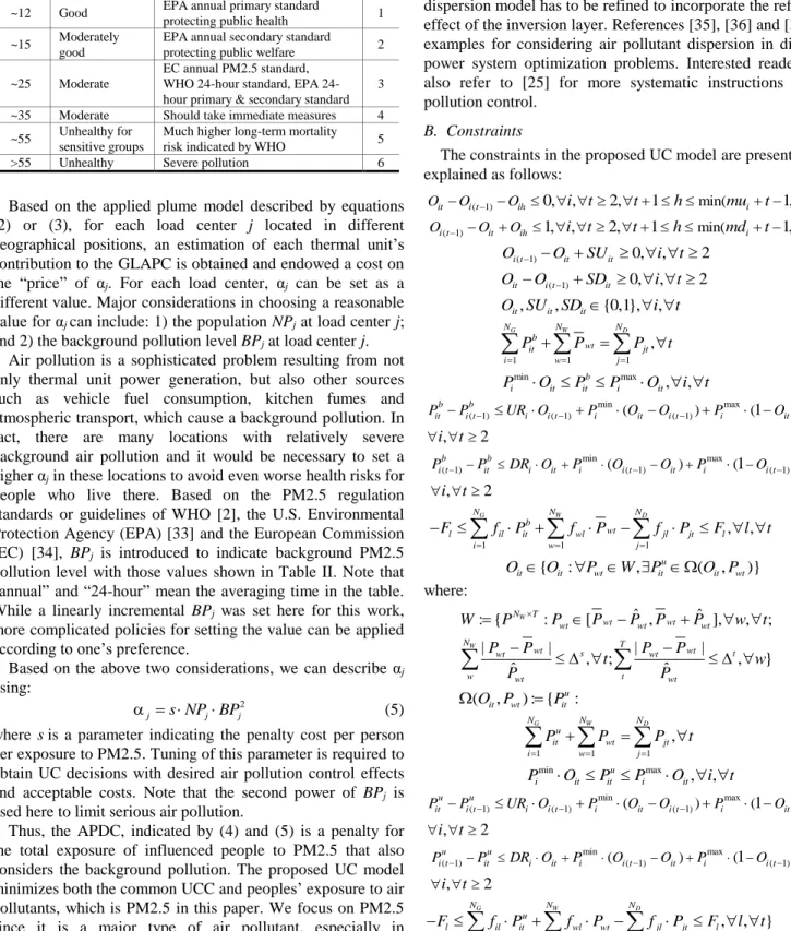
AIR QUALITY STANDARDS FOR PM2.5 AND SETTING BPj PM2.5
μg/m3
Air quality
category Remarks BPj
~12 Good EPA annual primary standard
protecting public health 1 ~15 Moderately
good
EPA annual secondary standard protecting public welfare 2 ~25 Moderate
EC annual PM2.5 standard, WHO hour standard, EPA 24-hour primary & secondary standard
3 ~35 Moderate Should take immediate measures 4 ~55 Unhealthy for
sensitive groups
Much higher long-term mortality
risk indicated by WHO 5
>55 Unhealthy Severe pollution 6
Based on the applied plume model described by equations (2) or (3), for each load center j located in different geographical positions, an estimation of each thermal unit’s contribution to the GLAPC is obtained and endowed a cost on the “price” of αj. For each load center, αj can be set as a
different value. Major considerations in choosing a reasonable value for αj can include: 1) the population NPj at load center j;
and 2) the background pollution level BPj at load center j.
Air pollution is a sophisticated problem resulting from not only thermal unit power generation, but also other sources such as vehicle fuel consumption, kitchen fumes and atmospheric transport, which cause a background pollution. In fact, there are many locations with relatively severe background air pollution and it would be necessary to set a higher αj in these locations to avoid even worse health risks for
people who live there. Based on the PM2.5 regulation standards or guidelines of WHO [2], the U.S. Environmental Protection Agency (EPA) [33] and the European Commission (EC) [34], BPj is introduced to indicate background PM2.5
pollution level with those values shown in Table II. Note that “annual” and “24-hour” mean the averaging time in the table. While a linearly incremental BPj was set here for this work,
more complicated policies for setting the value can be applied according to one’s preference.
Based on the above two considerations, we can describe αj
using:
2
j s NP BPj j
(5) where sis a parameter indicating the penalty cost per person per exposure to PM2.5. Tuning of this parameter is required to obtain UC decisions with desired air pollution control effects and acceptable costs. Note that the second power of BPj is
used here to limit serious air pollution.
Thus, the APDC, indicated by (4) and (5) is a penalty for the total exposure of influenced people to PM2.5 that also considers the background pollution. The proposed UC model minimizes both the common UCC and peoples’ exposure to air pollutants, which is PM2.5 in this paper. We focus on PM2.5 since it is a major type of air pollutant, especially in developing countries, such as China.
Note that our method of air pollutant dispersion consideration can be easily extended to other pollutants such as PM10, NOX and SO2,as well as other problems such as ED and generation expansion planning. Generally, a dispersion model should be selected first according to the spatial and
temporal considerations of the studied or applied problem, followed by necessary modifications. Then the problem can be formulated and revised. For example, if the atmosphere is of the temperature inversion condition, the Gaussian plume dispersion model has to be refined to incorporate the reflection effect of the inversion layer. References [35], [36] and [37] are examples for considering air pollutant dispersion in different power system optimization problems. Interested readers can also refer to [25] for more systematic instructions on air pollution control.
B. Constraints
The constraints in the proposed UC model are presented and explained as follows: ( 1) 0, , 2, 1 min( 1, ) it i t ih i O O O i t t h mu t T (6) ( 1) 1, , 2, 1 min( 1, ) i t it ih i O O O i t t h md t T (7) ( 1) 0, , 2 i t it it O O SU i t (8) ( 1) 0, , 2 it i t it O O SD i t (9) , , {0,1}, , it it it O SU SD i t (10) 1 1 1 , G W D N N N b wt it jt i w j P P P t
(11) min b max , , i it it i it P O P P O i t (12) min max ( 1) ( 1) ( ( 1)) (1 ), , 2 b b it i t i i t i it i t i it P P UR O P O O P O i t (13) min max ( 1) ( ( 1) ) (1 ( 1)), , 2 b b i t it i it i i t it i i t P P DR O P O O P O i t (14) 1 1 1 , , G W D N N N b wt l il it wl jl jt l i w j F f P f P f P F l t
(15) { : , u ( , )} it it wt it it wt O O P W P O P (16) where: ˆ ˆ : { : [ , ], , ; | | | | , ; , } ˆ ˆ W W N T wt wt wt wt wt N T wt s wt t wt wt w wt t wt W P P P P P P w t P P P P t w P P
(17) ( , ) : { u: it wt it O P P 1 1 1 , G W D N N N u it wt jt i w j P P P t
(18) min u max , , i it it i it P O P P O i t (19) min max ( 1) ( 1) ( ( 1)) (1 ), , 2 u u it i t i i t i it i t i it P P UR O P O O P O i t (20) min max ( 1) ( ( 1) ) (1 ( 1)), , 2 u u i t it i it i i t it i i t P P DR O P O O P O i t (21) 1 1 1 , , } G W D N N N u l il it wl wt jl jt l i w j F f P f P f P F l t
(22)Among these constraints, inequalities (6)-(10) are constraints for commitment decision variables. Constraints (6) and (7) are minimum up-time and minimum down-time limits. Inequalities (8) and (9) are the logic constraints for start-up and shut-down operations, respectively. Constraint (10)
enforces commitment decision variables be binary. Constraints (11)-(15) are for base-case dispatch variables. Equation (11) represents the power balance for each time interval. Constraint (12) limits the power output of thermal units within its upper and lower bound. Constraints (13) and (14) indicate ramp-up and ramp-down rate limits. Inequality (15) is the power flow capacity constraints for the transmission lines. Constraint (16) is the robust feasibility check for the on/off state variables of the thermal units to guarantee existence of feasible adaptive dispatch strategies under any scenario within the wind power outputs’ uncertainty set W defined by (17). Here, Ω(Oit,Pit) is
the feasible set of adaptive dispatch variables indicated by (18)-(22). In (17), Δs is the “spatial budget” to limit wind
power deviations at each time interval t, while Δt is the
“temporal budget” to limit deviations during the whole time window for each wind farm w. Constraints (18)-(22) represent power balance, thermal unit power output limits, ramp-up and ramp-down rate limits, and transmission line capacities, respectively.
Specifically, the robust feasibility check constraint is added for two major reasons. First, wind power uncertainties have to be considered appropriately, so that adequate spinning reserve is set, to avoid over-estimating and in turn under-utilizing wind power benefits for air pollutant dispersion control. That is, if UC decisions are determined based on forecasted mean values of wind power outputs, inadequate spinning reserve can lead to frequent start-up/shut-down of flexible units and environmentally unfriendly real-time operations of more polluting coal-fired units, which can cause much higher operational costs and even worse air pollutant dispersion results. In such cases, wind power becomes cost-ineffective or even ineffective for air pollutant dispersion control. Second, here robust optimization [21]-[23], [38] is more appropriate compared to deterministic and stochastic optimization methods [39]-[40]. If the distribution information of uncertainties is available, which is often not the case, stochastic optimization can be preferable. Otherwise, instead of setting intuitive criteria based spinning reserve, robust optimization should be applied to optimally schedule spinning reserve, so that wind power benefits in air pollutant dispersion control can be estimated properly and thus utilized sufficiently.
IV. SOLUTION ALGORITHM
The proposed UC model results in a mixed integer quadratic programing (MIQP) problem with a robust feasibility check. For simplicity and clarity in presenting the solution algorithm, its compact matrix formulation is derived as:
, min T (1/ 2) T T 1 0 1 1 1 1 x y q x y Qy q y (23) . . + s t Rx Gy 1 Du0e (24) 2 , : u U y Ax By 2Eug (25) where x, y1, y2, u0, u, and U denote commitment variables,
base-case dispatch variables, adaptive dispatch variables, forecasted mean wind power outputs, uncertain wind power outputs, and their uncertainty set, respectively. Other vectors and matrices are cost parameters or coefficients in the constraints.
The solution algorithm is in an iterative master-sub-problem framework. First, the robust feasibility check (25) is implemented by a sub-problem (SP) written as:
SP: , , max min T T + - 2 + -u U y s s 1 s 1 s (26) s.t. K + - 2 Ax By Eu Is Is g (27) where I, 1, s+, s-, and x
K denote the identity matrix, all-ones
vector, positive slack vector, negative slack vector, and the current solution of x intheKthiteration, respectively.
The SP can be solved in one of two ways: 1) first taking the dual of the inner minimization problem and then linearizing the resulting bilinear terms in the objective function via McCormick envelopes [38], [41]; or 2) first employing the Karush-Kuhn-Tucker conditions for the inner minimization problem and then linearizing the complementary slackness constraints via big-M linearization [23], [42]. Both approaches lead to a mixed integer linear programming (MILP) problem that can be solved by off-the-shelf solvers such as Gurobi. We apply the first method in this work.
By dualizing the inner minimization problem and incorporating the derived dual formulation with the outer maximization problem, the SP becomes a bilinear program (BLP) sub-problem: BLP-SP: , max T( ) T K u U ηη g Ax η Eu (28) s.t. η B 0T T (29) T T T 1 η 0 (30) where η and 0 denote the dual variables and all-zero vector, respectively. As the BLP-SP is non-convex, its global optimum is difficult to obtain. Thus, we transform the problem into an equivalent MILP instead by first representing each uncertain variable um with:
ˆ )
m m m m m
u u (uu u (31) where um and uˆm denote the forecasted mean value and deviation of um, respectively, and um
and m
u are binary variables. The matrix E is sparse in our case. Then we eliminate each bilinear term in the BLP-SP by using an auxiliary continuous variable and four linear constraints. For example, the bilinear term mun can be represented by vmn and constrained by:
0, , , 1.
mn m mn n mn mn m n
v v u v v u (32) As in (32), the bounds for dual variables are explicitly known, so appropriately pre-specified big-M values are not necessary to linearize the BLP-SP. The resulting MILP is parameter-free.
If the objective of the SP is zero or less than a pre-set threshold δ, we conclude that the current xK satisfies the robust
feasibility check (25). Otherwise, based on the identified “worst scenario” uK, cuts should be added to form the
master-problem (MP) with (23)-(24) and previously added cuts: MP: ,min, k (1/ 2) T T T 1 2, 0 1 1 1 1 x y y q x y Qy q y (33) s.t. (24) ,k k , k K 2 Ax By Eu g (34)
Here, y2,k is the introduced dispatch variables under the
scenario uk. The MP is a MIQP problem with a positive
semi-definite Q matrix involving only positive diagonal elements. Thus, the MP can be efficiently solved by off-the-shelf solvers as well. Note that cuts can also be generated in terms of dual variables based on Benders cutting plane algorithms [21]-[22]. Here we add cuts in terms of primal variables based on the idea of the column-and-constraint generation (C&CG) algorithm [23], [42]. Although the C&CG algorithm adds not only more constraints but also new variables into the MP, it shows better performance in terms of computational time and required number of iterations [23], [42].
The iterative algorithm is presented as follows:
1) Set the number of iterations K=0. Choose a tolerance δ(>0) for the robust feasibility check.
2) Solve the MP to update the current optimal solution (x*,
y1*, y2,1*,…, y2,K*).
3) K=K+1. Solve the SP with xK=x*, to obtain uK.
4) If objective_of_SP≤δ, return (x*, y
1*) and terminate.
Otherwise, go to step 2).
Theoretically, the maximum iteration number of the above algorithm is the number of extreme points of the uncertainty set. However, this method normally acquires the optimum solution within several iterations.
V. ILLUSTRATIVE CASES
Case studies were conducted on a modified IEEE 14-bus system and the real-world Guangdong Grid system to demonstrate the need for air pollutant dispersion consideration and the effectiveness of the proposed UC model. Gurobi 6.0.4 was used to solve related MIQP and MILP problems.
A. The Modified IEEE 14-Bus System
This system has 5 thermal units, the data for which are shown in Table III. Note that gas units hardly emit any PM2.5. One wind farm with 10% penetration on average was introduced to bus 14, with its hourly forecasted mean power output and the system load given in Fig. 2. Wind power uncertainties were set as ±10% of forecasted values, with Δs=1
and Δt=16. Transmission line data were obtained from
MATPOWER [43]. The geographic distribution of the thermal units and load centers was based on [35]. The background PM2.5 pollution, and the corresponding BPj and NPj, are listed
in columns 1-4 in Table IV. As for meteorological conditions, we set the average wind speed and direction to be 4.2 m/s from the south during the day and 9.3 m/s from the southwest at night. The atmospheric stability class was set to D, i.e., neutral stability. This determines the two meteorological parameters Iy
and Iz to be 0.147 and 0.811, respectively.
Four cases were studied for illustration: Case 1: this case does not include the wind farm at bus 14, nor the APDC in the objective function; Case 2: in this case the wind farm is considered, while the APDC is still absent from the objective function; Case 3: a constraint for total PM2.5 emission is added based on Case 2; Case 4: the exact proposed UC model is applied for this case, where s is set as 0.01 $·m3/µg.
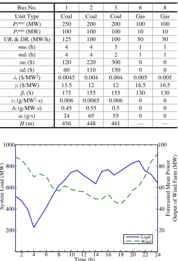
TABLEIII DATA FOR THERMAL UNITS
Bus No. 1 2 3 6 8
Unit Type Coal Coal Coal Gas Gas
Pimax(MW) 250 200 200 100 100 Pimin(MW) 100 100 100 10 10 URi & DRi(MW/h) 125 100 100 50 50 mui(h) 4 4 3 1 1 mdi(h) 4 4 2 1 1 sui($) 120 220 300 0 0 sdi($) 60 110 150 0 0 λi($/MW2) 0.0045 0.004 0.004 0.005 0.005 γi($/MW) 13.5 12 12 16.5 16.5 βi($) 175 155 155 130 130 ci(g/MW2·s) 0.006 0.0065 0.006 0 0 bi(g/MW·s) 0.45 0.55 0.5 0 0 ai(g/s) 24 65 55 0 0 H (m) 456 448 461 — — 2 4 6 8 10 12 14 16 18 20 22 24 200 400 600 800 1000 S y st em L o ad ( M W ) 20 100 Load Wind F o re ca st ed M ea n P o w er O u tp u t o f W in d F ar m ( M W ) 40 60 80 Time (h)
Fig. 2. System load profile and forecasted mean power outputs of the wind farm.
TABLEIV
LOAD CENTERBPj,NPj,PGLAPC AND AGLAPC FOR THE FOUR CASES
Bus No. Back-ground PM2.5 µg/m3 BPj NPj PGLAPCµg/m3 AGLAPCµg/m3
Case No. Case No.
1 2 3 4 1 2 3 4 4 22 3 9203 22.00 22.00 22.00 22.00 20.00 22.00 22.00 22.00 5 50 5 1463 70.32 70.32 64.79 56.07 59.97 59.15 56.04 52.53 7 22 3 320 22.00 22.00 22.00 22.00 22.00 22.00 22.00 22.00 9 22 3 5680 22.00 22.00 22.00 22.00 22.00 22.00 22.00 22.00 10 30 4 1733 30.02 30.02 30.02 30.01 30.01 30.01 30.00 30.00 11 36 5 674 53.28 53.28 53.28 53.28 46.14 46.01 46.13 46.75 12 23 3 1174 32.36 32.36 31.99 31.46 28.60 28.34 27.71 27.61 13 18 3 2600 21.02 21.02 20.97 20.90 20.57 20.37 19.73 19.97 14 13 2 2869 13.13 13.13 13.13 13.13 13.06 13.06 13.02 13.06
In Table IV, the resulting peak GLAPC (PGLAPC) and average GLAPC (AGLAPC) of each load center under the four cases are listed. In Table V, total PM2.5 emissions (TPME), total exposure (TE, sum of NPj·GLAPCjt for all load centers and
all time intervals), UCC, and the system’s PGLAPC and AGLPAC are shown. The on/off states of the thermal units under the four cases are given in Table VI, where the grey-colored data are the ones that are different between the cases. From these results, several points can be drawn:
TABLEV
COST AND EMISSION RESULTSFOR THE FOUR CASES (IEEE14-BUS SYSTEM) UCC k$ TPME ton PGLAPC µg/m3 AGLAPC µg/m3 TE ·105µg/m3 Case 1 224.58 100.25 70.32 29.37 150.92 Case 2 200.19 93.43 70.32 29.22 150.42 Case 3 213.38 65.00 64.79 28.29 148.09 Case 4 209.79 67.90 56.07 28.10 145.81 TABLE VI
ON/OFF STATE COMPARISON OF THE FOUR CASES
Hour
Case 1 Case 2 Case 3 Case 4
Unit Bus No. Unit Bus No. Unit Bus No. Unit Bus No. 1 2 3 6 8 1 2 3 6 8 1 2 3 6 8 1 2 3 6 8 1 1 1 1 0 0 0 1 1 1 0 1 0 0 1 1 0 1 1 0 1 2 1 1 1 0 0 0 1 1 1 0 1 0 0 1 1 0 1 1 0 1 3 0 1 1 0 0 0 1 1 1 0 1 0 0 1 1 0 1 1 0 1 4 0 1 1 0 0 0 1 0 1 0 1 0 0 1 1 0 1 0 0 1 5 0 1 1 0 0 1 1 0 0 0 1 0 0 1 1 0 1 0 0 1 6 0 1 1 1 1 1 1 1 0 0 1 0 0 1 1 0 1 1 1 1 7 1 1 1 1 0 1 1 1 0 0 1 0 1 1 1 0 1 1 1 1 8 1 1 1 1 0 1 1 1 0 0 1 0 1 1 1 0 1 1 1 1 9 1 1 1 1 0 1 1 1 0 1 1 0 1 1 1 1 1 1 1 1 10 1 1 1 1 1 1 1 1 0 1 1 1 1 1 1 1 1 1 1 1 11 1 1 1 1 1 1 1 1 0 1 1 1 1 1 1 1 1 1 1 1 12 1 1 1 1 1 1 1 1 0 1 1 1 1 1 1 1 1 1 1 1 13 1 1 1 0 1 1 1 1 0 1 1 1 1 0 1 1 1 1 1 1 14 1 1 1 0 1 1 1 1 0 1 1 1 1 0 1 1 1 1 1 1 15 1 1 1 1 1 1 1 1 0 1 1 1 1 0 1 1 1 1 1 1 16 1 1 1 1 1 1 1 1 0 1 1 1 1 1 1 1 1 1 1 1 17 1 1 1 1 1 1 1 1 0 1 1 1 1 1 1 1 1 1 1 1 18 1 1 1 1 1 1 1 1 0 1 1 1 1 1 1 1 1 1 1 1 19 1 1 1 1 1 1 1 1 1 1 1 1 1 1 1 1 1 1 1 1 20 1 1 1 1 1 1 1 1 1 1 1 1 1 1 1 1 1 1 1 1 21 1 1 1 1 1 1 1 1 1 1 1 1 1 1 1 1 1 1 1 1 22 1 1 1 1 1 1 1 1 1 1 1 1 1 1 1 1 1 1 1 1 23 1 1 1 1 1 1 1 1 1 0 1 0 1 1 1 1 1 1 1 1 24 1 1 1 1 0 1 1 1 0 0 1 0 1 1 1 0 1 1 1 1 0 2 4 6 8 10 12 50 60 70 AUCC (k$) P G L A P C ( µ g /m 3 ) 28 28.5 29 PGLAPC without wind AGLAPC without wind
A G L A P C ( µ g /m 3 ) PGLAPC with wind
AGLAPC with wind
Fig. 3. Curves of AUCC-PGLAPC and AUCC-AGLAPC with and without wind power (IEEE 14-bus system).
1)With wind power integrated, we still need to explicitly consider emissions during operations to utilize the benefits of wind power for air pollution control. Take Case 2 as an example, where TE and the system’s AGLAPC only decrease by 0.33% and 0.49%, respectively, compared to Case 1,
although TPME decreases due to 10% less power demand from the thermal units. The system’s PGLAPC stays the same at 70.32 µg/m3, which is classified as severe pollution. This is because the system still uses more power from cheaper but more polluting coal units, as indicated in Table VI.
2)The measure for limiting the total amount of air pollutant emissions, i.e., TPME in this paper, can be less cost-effective than our proposed method in terms of air pollution control with wind power integration. From Cases 3 and 4, we can see that, if emission is explicitly considered, wind power is helpful in improving the effects of air pollution control. However, comparing Case 4 to Case 3, the results of the system’s PGLAPC, AGLAPC, and TE are 13.46%, 0.67%, and 1.54% better, respectively, with $3590 less UCC in Case 4. Note that in Case 3, TPME is limited to 65 tons, which is actually less than that of Case 4. This demonstrates our argument that meteorological conditions and the system’s geographical distribution are critical factors for environmental generation scheduling.
3) Our proposed UC model can be quite helpful in realizing wind power benefits in air pollution control, especially for a system with locations with severe background pollution. In this system, the load center on bus 5 had the highest background PM2.5 concentration. Cases 1, 2, and 3 all resulted in much worse PGLAPC and AGLAPC, while in Case 4 they were both much lower. As shown in Table VI, the coal unit at bus 1, which is exactly in the upwind direction of bus 5, is turned on much less in Case 4 to ensure better air quality for the load center on bus 5. Compared to Case 3, this leads to a relatively slight increase in AGLAPC for the load centers on buses 11, 13, and 14, where the background PM2.5 pollutions are not as severe as at the load center on bus 5. This is an acceptable compromise.
We further explored the cost and effectiveness of reducing a system’s PGLAPC and AGLAPC with and without wind power. First, based on Case 4, s was gradually increased from 0.0001 to 0.1 $·m3/µg, to obtain relationships between additional UCC (AUCC) and the PGLAPC, as well as between the AUCC and the AGLAPC.TheAUCCistheincreasedUCC comparedtoCase 2. Secondly, similar work was done with wind power outputs set to zero such that the AUCC became the increased UCC compared to Case 1. As shown is Fig. 3, the system can be much more cost-effective in reducing the PGLAPC and AGLAPC when wind power is accommodated and proper consideration is given to air pollutant dispersion. This capability is also strengthened by wind power, since both the convergent PGLAPC and AGLAPC with AUCC increased are smaller with wind power compared to without wind power. These quantitative relationships can guide system operators in environmental generation scheduling according to their cost budget and air pollution control objective, and help governments in making corresponding subsidies or tax policies for air pollution control.
B. The Guangdong Grid System
The Guangdong Grid system has 1117 buses and 116 thermal units, with 6 planned wind farms reaching about 15% penetration. Reducing air pollution (GLAPC) in Guangzhou was the focus of this simulation. Monitored locations were
TABLEVII
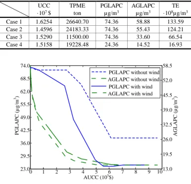
COST AND EMISSION RESULTSOF THE FOUR CASES (GUANGDONG GRID) UCC ·107 $ TPME ton PGLAPC µg/m3 AGLAPC µg/m3 TE ·108µg/m3 Case 1 1.6254 26640.70 74.36 58.88 133.59 Case 2 1.4596 24183.33 74.36 55.43 124.21 Case 3 1.5290 11500.00 74.36 33.60 66.54 Case 4 1.5158 19228.48 24.36 14.52 16.93 23.0 29.5 36.0 42.5 49.0 55.5 62.0 68.5 74.0 0 1 2 3 4 5 6 7 8 9 1013.0 19.5 26.0 32.5 39.0 45.5 52.0 58.5 PGLAPC without wind AGLAPC without wind PGLAPC with wind AGLAPC with wind
AUCC (105 $) P G L A P C ( µ g /m 3) A G L A P C ( µ g /m 3)
Fig. 4. Curves of AUCC-PGLAPC and AUCC-AGLAPC with and without wind power (Guangdong Grid)
selected among its 11 districts. The simulation assumed a summer day with a 2.44m/s southeast wind and neutral atmospheric stability. The applied plume model was also
modified to consider the special temperature inversion condition prevalent in the area. Based on the meteorological and geographical conditions, 44 coal units out of the total 116 units were identified as directly influencing the GLAPC in Guangzhou and were specifically considered for air pollutant dispersion control. The other units in the system were only included in the UC model for on/off operational planning.
Similar to the previous study, four cases were simulated, with the TPME limit of Case 3 and s of Case 4 set as 11500.00 tons and 0.003 $·m3/µg, respectively. A part of results are shown in Table VII and Fig. 4. Note that the PGLAPC and AGLAPC in cases 1, 2 are over 70 and 55 µg/m3, respectively, which are values actually seen in Guangzhou on some summer days. In Case 2, air pollution is not quite relieved by integrated wind power, although the AGLAPC decreases slightly. This again demonstrates the need to explicitly consider emission issues for air pollution control. As indicated by Case 3, only limiting TPME is not an effective measure in air pollution control. In Case 4, the proposed UC model explicitly considers the dispersion of emitted air pollutants, resulting in better air pollution control with less cost,aswind power’s environmental benefits are better realized. Fig. 5 again proves that wind power makes a system more cost-effective and more capable of air pollution control.
Note that this paper studied measures for limiting total emissions and the proposed method separately for comparison. In practice, both have to be considered, since total emissions are mostly limited by laws or regulations. The proposed method will help to achieve better and more cost-effective air pollution control in this case.
VI. CONCLUSIONS
This paper proposed a UC model that considered the dispersion of air pollutants emitted by thermal units via a plume model involving meteorological conditions and the system’s geographical distribution to utilize wind power benefits in air pollution control. The GLAPC at monitored locations was modeled and rendered a cost to achieve the spatial distribution control of air pollutants. Robust optimization was applied to appropriately accommodate wind power uncertainties in terms of spinning reserve scheduling, so that the benefits of wind power for air pollutant dispersion control could be properly estimated and sufficiently utilized. Illustrative cases showed that wind power benefits in air pollution control should be explicitly considered as they were not fully utilized by only limiting total air pollutants emissions. This highlights the need to consider air pollutant dispersion. The proposed model proved to be quite effective in controlling air pollution, utilizing wind power benefits, and providing useful information for system operators and policy-makers to conduct environmental generation scheduling. We also showed that wind power makes a system more cost-effective and more capable of air pollution control. For future research, it may be beneficial to develop an intro-day economic dispatch framework to consider localized meteorological conditions, which are unknown or only known with great uncertainty in day ahead scheduling but which are available in real time or near real-time.
VII. REFERENCES
[1] United Nations Envieonment Programme, “UNEP Year Book 2014 Emerging Issues Update,” 2014.
[2] World Health Organization, “WHO Air Quality Guidelines—Global Update 2005,” 2005.
[3] M. J. Leppitsch and B. F. Hobbs, “The effect of NOx regulations on emissions dispatch: a probabilistic production costing analysis,” IEEE Trans. Power Syst., vol. 11, no. 4, pp. 1711-1717, Nov. 1996.
[4] J. H. Talaq, F. El-Hawary, and M. E. El-Hawary, “A summary of environmental/economic dispatch algorithms,” IEEE Trans. Power Syst.,
vol. 9, no. 3, pp. 1508-1516, Aug. 1994.
[5] R. Ramanathan, “Emission constrained economic dispatch,” IEEE Trans. Power Syst., vol. 9, no. 4, pp. 1994-2000, Nov. 1994.
[6] M. R. Gent, and J. W. Lamont, “Minimum-Emission Dispatch,” IEEE Trans. Power App. Syst., vol. PAS-90, no. 6, pp. 2650-2660, Nov. 1971. [7] R. Tong and J. Keenan, “Economic Dispatch for Flue Gas
Desulfurization," J. Energy Eng., vol. 109, no. 1, pp. 17-34, 1983. [8] K. C. Chu, M. Jamshidi, and R. E. Levitan, “An approach to on-line
power dispatch with ambient air pollution constraints,” IEEE Trans. Autom. Control, vol. 22, no. 3, pp. 385-396, Jun. 1977.
[9] P. Dejax and D. C. Gazis, “Optimal dispatch of electric power with ambient air quality constraints,” IEEE Trans. Autom. Control, vol. 21, no. 2, pp. 227-233, Apr. 1976.
[10] P. F. Schweizer, “Determining optimal fuel mix for environmental dispatch,” IEEE Trans. Autom. Control, vol. 19, no. 5, pp. 534-537, Oct. 1974.
[11] V. C. Gungor, D. Sahin, T. Kocak, S. Ergut, C. Buccella, C. Cecati, and G. P. Hancke., "Smart Grid Technologies: Communication Technologies and Standards," IEEE Trans. Ind. Informat., vol. 7, pp. 529-539, Nov. 2011. [12] Global Wind Energy Council, “Global Wind Report 2013,” 2014. [13] F. Yao, Z. Y. Dong, K. Meng, Z. Xu, H. H. C. Iu, and K. P. Wong,
"Quantum-Inspired Particle Swarm Optimization for Power System Operations Considering Wind Power Uncertainty and Carbon Tax in Australia," IEEE Trans. Ind. Informat., vol. 8, pp. 880-888, Nov. 2012. [14] Y. Zhang, H. H. C. Iu, T. Fernando, F. Yao, and K. Emami, "Cooperative Dispatch of BESS and Wind Power Generation Considering Carbon Emission Limitation in Australia," IEEE Trans. Ind. Informat., vol. 11, pp. 1313-1323, Dec. 2015.
[15] C. Wang, Z. Lu, and Y. Qiao, “A Consideration of the Wind Power Benefits in Day-Ahead Scheduling of Wind-Coal Intensive Power Systems,”IEEETrans.PowerSyst.,vol.28,no.1,pp.236-245,Feb. 2013.
[16] S. H. Madaeni, and R. Sioshansi, “Using Demand Response to Improve the Emission Benefits of Wind,” IEEE Trans. Power Syst., vol. 28, no. 2, pp. 1385-1394, May 2013.
[17] E. Denny and M. O'Malley, “Wind generation, power system operation, and emissions reduction,” IEEE Trans. Power Syst., vol. 21, no. 1, pp. 341-347, Feb. 2006.
[18] X. Liu and W. Xu, “Minimum Emission Dispatch Constrained by Stochastic Wind Power Availability and Cost,” IEEE Trans. Power Syst., vol. 25, no. 3, pp. 1705-1713, Aug. 2010.
[19] B. F. Hobbs, M. C. Hu, Y. Chen, J. H. Ellis, A. Paul, D. Burtraw, and K. L. Palmer, “From Regions to Stacks: Spatial and Temporal Downscaling of Power Pollution Scenarios,” IEEE Trans. Power Syst., vol. 25, no. 2, pp. 1179-1189, May 2010.
[20] A. Trivedi, D. Srinivasan, K. Pal, C. Saha, and T. Reindl, "Enhanced Multiobjective Evolutionary Algorithm Based on Decomposition for Solving the Unit Commitment Problem," IEEE Trans. Ind. Informat., vol. 11, pp. 1346-1357, Dec. 2015.
[21] R. Jiang, J. Wang, and Y. Guan, "Robust Unit Commitment With Wind Power and Pumped Storage Hydro,", IEEE Trans. Power Syst., vol. 27, no. 2, pp. 800-810, May 2012.
[22] D. Bertsimas, E. Litvinov, X. A. Sun, J. Y. Zhao, and T. X. Zheng, "Adaptive Robust Optimization for the Security Constrained Unit Commitment Problem," IEEE Trans. Power Syst., vol. 28, no. 1, pp. 52-63, Feb. 2013.
[23] Y. An and B. Zeng, "Exploring the Modeling Capacity of Two-Stage Robust Optimization: Variants of Robust Unit Commitment Model,"
IEEE Trans. Power Syst., vol. 30, no. 1, pp. 109-122, Jan., 2015. [24] C. Peng, S. Lei, Y. Hou, and F. F. Wu, “Uncertainty Management in
Power System Operation,” CSEE J. Power Energy Syst., vol. 1, no. 1, pp. 28-35, Mar. 2015.
[25] N. de Nevers, Air Pollution Control Engineering, 2nd ed. Long Grove, Illinois, USA: Waveland Press, 2010.
[26] Environmental Protection Agency (U.S.), “AERMOD Implementation Guide,” 2015.
[27] Environmental Protection Agency (U.S.), “AERMOD: Description of Model Formulation,” 2004.
[28] Environmental Protection Agency (U.S.), “Documentation of the Evaluation of CALPUFF and Other Long Range Transport Models Using Tracer Field Experiment Data,” 2012.
[29] Environmental Protection Agency (U.S.), “Technical Issues Related to Use of the CALPUFF Modeling System for Near-field Applications,” 2008. [30] R. Lu and R. P. Turco, “Air pollutant transport in a coastal
environment—II. Three-dimensional simulations over Los Angeles basin,” Atmos. Environ., vol. 29, no. 13, pp. 1499-1518, 1995. [31] M. Y. Tsai and K. S. Chen, “Measurements and three-dimensional
modeling of air pollutant dispersion in an Urban Street Canyon,” Atmos. Environ., vol. 38, no. 35, pp. 5911-5924, Nov. 2004.
[32] X. Yang, F. Teng, and G. Wang, “Incorporating environmental co-benefits into climate policies: A regional study of the cement industry in China,” Applied Energy, vol. 112, pp. 1446-1453, Dec. 2013.
[33] Environmental Protection Agency (U.S.), “National Ambient Air Quality Standards,” 2012.
[34] European Commission, “Air quality standards,” 2010.
[35] Y. Hou, X. Wang, K. Liu, Z. Qin, and C. Wang, "Generation dispatch with air pollutant dispersion consideration," in Proc. IEEE Power and Energy Soc. General Meeting, Jul. 21-25, 2013, pp. 1-5.
[36] S. Lei, Y. Hou, X. Wang, and K. Liu, “Robust Generation Dispatch with Wind Power Considering Air Pollutant Dispersion,” in Proc. of 5th IEEE PES Innovative Smart Grid Tech. Conf. (ISGT), Washington, DC, Feb. 2014.
[37] S. Lei, Y. Hou, Z. Qin, and C. Peng, “Considering Geographical Distribution of Pollutants Emission in Production Costing,” in Proc. of 2015 IEEE PES General Meeting, Denver, CO, Jul. 2015.
[38] W. Wei, F. Liu, S. Mei, and Y. Hou, "Robust Energy and Reserve Dispatch under Variable Renewable Generation," IEEE Trans. Smart Grid, vol. 6, no. 1, pp. 369-380, Jan. 2015.
[39] M. Black and G. Strbac, “Value of bulk energy storage for managing wind power fluctuations,” IEEE Trans. Energy Convers., vol. 22, no. 1, pp. 197–205, Mar. 2007
[40] F. Bavafa, T. Niknam, R. Azizipanah-Abarghooee, and V. Terzija, "A New Bi-Objective Probabilistic Risk Based Wind-Thermal Unit Commitment Using Heuristic Techniques," IEEE Trans. Ind. Informat., in press (early access).
[41] G. P. McCormick, “Computability of global solutions to factorable nonconvex programs: Part I—Convex underestimating problems,”
Math. Program., vol. 10, no. 1, pp. 147–175, 1976.
[42] B. Zeng and L. Zhao, “Solving two-stage robust optimization problems using a column-and-constraint generation method,” Oper. Res. Lett., vol. 41, no. 5, pp. 457–461, Sep. 2013.
[43] R. D. Zimmerman, C. E. Murillo-Sánchez, and R. J. Thomas, "MATPOWER: Steady-State Operations, Planning and Analysis Tools for Power Systems Research and Education," IEEE Trans. Power Syst., vol. 26, no. 1, pp. 12-19, Feb. 2011.
Shunbo Lei (S’14) received the B.E. degree from Huazhong University of Science and Technology, Wuhan, China, in 2013. He is currently pursuing the Ph.D. degree with The University ofHong Kong, Hong Kong. He is currently visiting Argonne National Laboratory, Argonne, IL, USA. His research interests include operation optimization, environmental dispatch, resilience, and renewables integration of power systems.
Yunhe Hou (M’08-SM’15) received the B.E. and Ph.D. degrees in electrical engineering from Huazhong University of Science and Technology, Wuhan, China, in 1999 and 2005, respectively.
He was a Post-Doctoral Research Fellow at Tsinghua University, Beijing, China, from 2005 to 2007, and a Post-Doctoral Researcher at Iowa State University, Ames, IA, USA, and the University College Dublin, Dublin, Ireland, from 2008 to 2009. He was also a Visiting Scientist at the Laboratory for Information and Decision Systems,Massachusetts Institute of Technology, Cambridge, MA, USA, in 2010. He joined the faculty of the University of Hong Kong, Hong Kong, in 2009, where he is currently an Assistant Professor with the Department of Electrical and Electronic Engineering.
Dr. Hou is an Editor of the IEEE Transactions on Smart Grid and an Associate Editor of Journal of Modern Power Systems and Clean Energy.
Xi Wang received the B.E. and M.E. degrees from Tsinghua University, Beijing, China, in 2001 and 2007, respectively, and Ph.D. degree from The University of Hong Kong, Hong Kong, in 2011, all in environmental engineering.
She joined the South China Normal University, Guangzhou, China, in 2012, where she is currently an Assistant Professor with the School of Chemistry and Environment. Her research interests include in air pollution modeling and photocatalytic process.
Kai Liu received the B.Sc. degree from Tsinghua University, Beijing, China, in 2005, and the M.Phil. and Ph.D. degrees from The University of Hong Kong, Hong Kong, in 2007 and 2011, respectively, both in electrical engineering. He currently works as a senior engineer in the dispatch and control center of the China Southern Power Grid (CSG). His research interests include the operations, economics, and planning of power systems.