Synchronization for a DVB-T Receiver in Presence of Strong Interference
R. Mhiri
1, D. Masse
1, D. Schafhuber
21TDF-C2R,
1, Rue Marconi, Technopôle Metz 2000 57078 Metz Cedex 3, France Tel: +33 3 87 20 75 82, email: [email protected]
2Institute of Communications and Radio-Frequency Engineering, Vienna University of Technology Gusshausstrasse 25/389, A-1040 Vienna, Austria
Tel.: +43 1 58801 38973, web: www.nt.tuwien.ac.at, email: [email protected]
ABSTRACT
We consider synchronization of a multi-antenna receiver for terrestrial digital video broadcasting (DVB-T) in the presence of strong co-channel interference. Thereby, we use a detection approach to find the symbol starts from the received orthogonal frequency division multiplexed (OFDM) signals. We propose two algorithms that exploit different features of the DVB-T signal. Both algorithms take advantage from the spatial diversity provided by the antenna array. By simulations we demonstrate that the proposed algorithms show promising performance in presence of strong co-channel interference. The synchronization algorithms developed are applied in an interference analysis tool for DVB-T networks.
I. INTRODUCTION
DVB-T [1] is the European standard for terrestrial digital video services and the physical layer is based on OFDM [2]. With the deployment of DVB-T networks, co-channel interference problems may appear. The objective of the IST project ANTIUM is to develop a prototype interference analysis tool that permits the identification of all co-channel DVB-T transmitters interfering at the measurement location. Thereby, it is necessary to detect all DVB-T transmitters present in the received signal. Furthermore, for the demodulation, knowledge about the OFDM symbol start is required. We devise two synchronization algorithms with substantially improved performance compared to the conventional synchronization procedures for OFDM that rely on the cyclic prefix [3],[4], or, additionally, exploit the knowledge of the pilot symbols [5]. However, the conventional synchronization algorithms concern single antenna receivers only and, thus, cannot exploit the advantages of the antenna array. In this paper, we show how spatial diversity can be exploited for synchronization by using a detection approach. The proposed algorithms will be compared with the synchronization procedure described in [6].
The paper is organized as follows. In Section II we introduce the system model, in Section III we devise the proposed algorithms, and in Section IV we present the simulation results.
II. SYSTEM MODEL
We consider T interfering DVB-T transmitters.
Each transmitted signal is OFDM modulated with N
subcarriers and a cyclic prefix of length G [2]. From the
subcarriers, about 10% are used to transmit pilot symbols. These pilot subcarriers are modulated with a known reference sequence. In DVB-T continual pilots and scattered pilots are multiplexed into the transmit data stream [1]. The continual pilots are always transmitted at the same subcarrier (frequency location). For the scattered pilots the subcarrier location varies in periods of 4 OFDM symbols.
For the time-varying multipath vector channel we used Clarkes’s model [7]. The base-band received signal for one DVB-T transmitter is
( )
∑
(
)
= − = P p p pd t a t 1 τ x(
)
− + ⋅∑
= np np np N n p n j c P , , , 1 , exp 2 cosθ γ ϕ S λ ν π (1)wherex(t) is the received signal vector of size M (the
number of antennas), d(t) is the DVB-T transmitted
signal, P is the number of paths, ap is the attenuation of
the pth path, τp is the delay of the pth path, Np is the
number of elementary sub-paths associated to the pth
path, cn,p is the attenuation of the nthsub-path associated
to the pth path, v is the mobile speed, γ is the angle
between the mobile speed and the North (randomly uniformly distributed in [0,2π]), λ is the wavelength, θn,p is the azimuth of the nth sub-path associated to the pth path, ϕn,p is the phase of the nth sub-path associated
to the pth path (randomly uniformly distributed in [0,2π
]), and Sn,p is the steering vector of the nth sub-path
associated to the pth path.
III. SYNCHRONIZATION ALGORITHMS
The time synchronization algorithms presented here exploit the spatial diversity provided by the antenna array. The basic idea is to implement a spatial filter (or a space-time filter) and to calculate a detection statistics using the output of the filter. The detection statistics is then compared to a threshold to validate the presence of
one or several DVB-T signals. Two algorithms are developed in this section (see below).
1. Correlation with Known Sequence
The first algorithm is adapted from [8] and [9] to the DVB-T case. It relies on the detection of a known reference sequence d(k) of length Nd.
We consider the following hypotheses test: H1: x(n+k)=hd(k)+w(n+k) (2)
H0: x(n+k)=w(n+k) (3)
for n = 0,1,..., Nr-1 and k = 0, 1, …, Nd-1. Here, w(n) is
assumed to be spatially correlated and temporally white interference and noise. Furthermore, we assume that the channel consists only of a single path h, Nr is the length
of the received sequence, and Ndis the length of the
reference sequence. We use as detection statistics the maximum likelihood ratio which can be shown to be
( )
( ) ( ) ( )
n n n d n c d H d xx x x R r rˆ ˆ ˆ 2 1 −1 = (4) where∑
−( )
= = 1 0 2 2 Nd k k d d (5)( )
∑
−(
) ( )
= + = 1 0 * ˆ Nd k d n xn k d k rx (6)( )
∑
−(
) (
)
= + + = 1 0 ˆ Nd k H n k k n n x x Rxx (7)The expression (4) can be interpreted as the correlation of the reference sequence with the spatially filtered received signal. The spatial filter is matched to the reference sequence. The detection statistics (4) has a dominant peak at the synchronization position n0.
In DVB-T, the time domain sequence stemming from the pilot subcarriers (continual and/or scattered pilots) can be used. However, this reference sequences have the drawback that they exhibit poor correlation properties. Indeed, the detection statistics (4) has many secondary peaks that do not correspond to a synchronization position of a DVB-T transmitter. Since we know the locations of these secondary peaks relatively to the position of the dominant peak, the secondary peaks can be discarded after the detection of a main peak.
2. Correlation with Cyclic Prefix
This second algorithm is an extension of [4] to the antenna array case. Here, we calculate a spatial filter
g(n) that maximizes the cross-correlation with the cyclic
prefix under a suitably chosen side constraint. The detection statistics is
( )
1(
( ) (
)
)
(
( ) (
)
)
2 0 * ) ( max∑
− = + + + = G i H H n N i n n i n n n c g x g x g (8)where the maximization is carried out either under the constraint g
( ) ( )
n Hgn =1 (9) or the constraint( ) (
)
( ) (
)
1 1 0 2 2 = + + + +∑
− = G i H H N i n n i n n x g x g (10)It can be shown that the equivalent formulation of the decision statistic (8) and the constraints (9) and (10) is
( )
( ) ( )
( )
( ) ( )
2 2 ) ( max ) ( n n n n n n n c H CP H n g R g g R g xx g = (11)where the sample cross-correlation matrix is
( )
∑
−(
) (
)
= + + + = 1 0 G i H CP n xn ix n i N R , (12)for the constraint (9) the sample correlation matrix is Rxx
( )
n =IM (13)and for the constraint (10) the sample correlation matrix is
( )
∑
−(
) (
)
= + + + = 1 0(
G i H n i i n n x x Rxx x(
n+i+N) (
xH n+i+N)
)
(14)The exact solution of (11) is difficult to find since the matrix RCP(n) in the numerator of (11) is in general
not an Hermitian matrix. However, we can show that an approximate solution to (11) is obtained by choosing for
( )
ng the eigenvector that corresponds to the maximum
eigenvalue of the Hermitian matrix
( )
= −1( )
(
( )
+( )
)
+ n n n n H CP CP R R R A xx(
( )
(
( )
H( )
)
)
H CP CP n n n R R Rxx + −1 (15)Then the detection statistics (11) is the maximum eigenvalue of (15) (in the following, we term this the synchronization criterion 1).
Alternatively, we will consider the following ad-hoc detection statistics (in the following referred to by synchronization criterion 2) ( )
( )
1( )
( ) ( )
2 n n n n n c = g H Rxx− RCP g (16)where g(n) is again the eigenvector associated to the
dominant eigenvalue of (15).
3. Integration of Detection Statistics
Similarly to the detection statistics (4), we can derive a statistics that takes into account the periodicity of the reference sequence Tsp using the hypotheses test :
H1: x(n+mTsp)=hd(n)+w(n+mTsp) (17) H0: x(n+mTsp)=w(n+mTsp) (18)
for m=0, …, Nsp-1, where Nsp is the number of observed
synchronization periods. It can be shown that the detection statistics for a maximum likelihood ratio test is
∑
−(
)
= + − − = 1 0 ) ( 1 ln 1 ) ( ~ Nsp m sp sp mT n c N n c (19) with c(n) given by (4).If all terms c(n+mTsp)in (19) are small compared to
1, the test statistics (19) is well approximated by
( )
∑
−(
)
= + = 1 0 1 Nsp m sp sp mT n c N n c (20)It is seen that (20) is an averaging of the synchronization criterion (4) over several periods. This will improve the detection probability while reducing the false alarm probability.
We note that averaging as in (20) can also be used with the detection statistics (8) and (16).
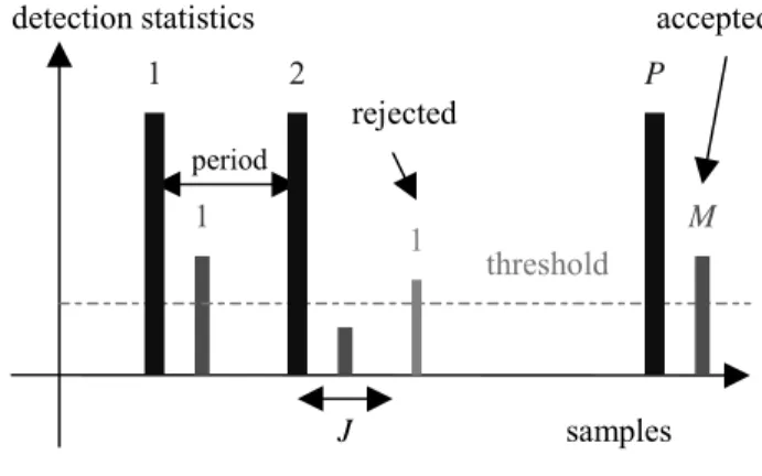
4. Rejection of False Alarms
The comparison of one of the detection statistics to a threshold can either result in the detection of the beginning of an OFDM symbol, or is a false alarm. We again use the periodicity of the detection statistics to reject false alarms. The peaks in the detection statistics corresponding to the beginning of an OFDM symbols appear every N+G samples (the total length of the
OFDM symbol) when we use the continual pilots as reference sequence and every 4(N+G) samples if we use
the scattered pilots. Thus, this peaks are regularly spaced, whereas peaks that would lead to false alarms appear randomly. Therefore, we only keep peaks that appear at least M times when considering P consecutive
OFDM symbols. Others are discarded. Furthermore,
these M peaks have to be regularly spaced with an
allowed jitter less than J samples. This strategy is
sketched in Figure 1.
Figure 1 : Rejection of false alarms
Denoting Pfas as the initial false alarm probability
obtained by applying one of the previously discussed synchronization algorithms and denoting as Pfat the
false alarm probability obtained after this rejection process, we have the relation
∑− ( ) ( ) − = − − − − − − = 1 1 1 . 1 1 . 1 1 . P M i P i C i P N s Pfa i N s Pfa s Pfa t Pfa (21)
Using similar notation for the detection probabilities, we have ∑−
[ ] [
]
− = − − − − = 1 1 1 . 1 1 . . P M i P i C i P s Pbd i s Pbd s Pbd t Pbd (22) IV. SIMULATIONS A. Simulation EnvironmentThe DVB-T standard specifies several values for the signal bandwidth as well as many configuration parameters. This allows DVB-T to cope with more or less severe propagation channels by adapting the useful bitrate, the robustness of the modulation, and the error protection level. We simulated the configuration that will be used in France. For this configuration, we have the parameters N=8192 and G=256. Therefore, for
the detection statistics (4), Nd can either be Nd = 8448 if
we use the continual pilots, or Nd = 4*8448 if we use the
scattered pilots. The receiver has a circular antenna array with M=5 sensors.
For the simulations we considered two scenarios. The first scenario consists of two co-channel interfering DVB-T transmitters. One DVB-T transmitter is transmitted over channel 2 (cf. Table 1). The other (interfering) DVB-T transmitter sends over channel 1 (cf. Table 1) and has a relative delay of (109 + n*924)
µs, where n is an integer.
The second scenario consists of three co-channel interfering DVB-T transmitters. One DVB-T transmitter sends over channel 4 (cf. Table 1). The dominant interfering DVB-T transmitter sends over channel 3 (cf. Table 1) and has a relative delay of (328 + n1*924) µs, where n1 is an integer. The other interfering DVB-T transmitter sends over channel 1 with a relative delay of (109 + n2*924) µs, where n2 is an integer, and its power is 10 dB below the power of the dominant interferer. The channels used in the simulations are Rayleigh multi-path channels with different gains applied to the different paths. The number of paths and the maximum delay for the different channels are summarized in Table 1. Channel Number of paths Maximum delay in µµµµs Channel 1 6 5 Channel 2 6 3.25 Channel 3 17 5.42 Channel 4 19 5.43
Table 1 : Channel characteristics used in the simulations
Further, for all channels and all paths we used 10 sub-paths with equal power. Phases and angles of arrival samples detection statistics 1 2 P J threshold M 1 rejected period 1 accepted
were randomly chosen in [0,2π] from an uniform distribution. With C/N, C/I, and I/N we denote the signal-to-noise ratio, the signal-to-interference ratio, and the interference-to-noise ratio, respectively.
The presented simulation results show the performances of the synchronization algorithms in terms of detection probability for a certain tolerable false alarm probability. Firstly, we evaluated the false alarm probability versus the threshold. Secondly, we evaluated the detection probability versus the false alarm probability.
The performances of the proposed algorithms will also be compared to the performances of a mono-sensor receiver and to the performances of the algorithm presented in [6].
B. Simulation Description
In order to evaluate the false alarm probabilities versus the thresholds we generate DVB-T signals with the following characteristics depending on the algorithm used :
• For the first synchronization algorithm, the signal has no continual and no scattered pilots.
• For the second synchronization algorithm, the
signal has no cyclic prefix.
For the first scenario, signals with these characteristics are used with C/I = 0 dB and C/N = 30 dB. For the second scenario, all three DVB-T transmitters have the same power and C/N = 30 dB. For each algorithm, we compute 5 times the corresponding detection statistics for a signal with length 12*8448 and average to reduce the influence on the actual channel parameters (angles of arrival, phase differences, etc.). For a predetermined list of thresholds, we count how often the criterion is larger than the threshold. Thus, we have a relation Pfas = f(threshold). The probability Pfat can be deduced from (21).
In order to evaluate the detection probability, we generate signals corresponding to each scenario. The channels are generated 14 times with different values for the angles of arrival and phases. The total duration corresponds to about 100 synchronization periods for each configuration. For each generation, we evaluate the values of the synchronization criterion at the positions of all the paths of the useful transmitter. For all studied scenarios, the I/N level was 20 dB and the C/I level was varied.
This information allows to evaluate the detection probabilities by comparing the values of the synchronization criteria to the thresholds.
C. Simulation Results
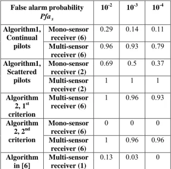
The Table 2 and Table 3 show the results for the detection probabilities corresponding to false alarm probabilities Pfas equal to 10-2, 10-3 or 10-4. The results obtained with the different algorithms are shown for both scenarios considering a C/I of -20 dB and a mobile
speed of 20 m/s. In each case, the detection probability is that of the path that is most often detected. In the tables, the values between parentheses represent the integration duration of the criterion in number of synchronization periods.
We can clearly see the improvement of the proposed algorithms for the multi-antenna receiver compared to the single antenna algorithms. In fact, the spatial filtering aims at rejecting the interfering signals. Such an anti-jamming processing is not possible with a mono-sensor receiver.
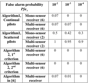
For all algorithms, scenario 2 is much more challenging than scenario 1. This is due to the supplementary interfering DVB-T transmitter as well as to the higher number of paths for each considered propagation channel. Both decrease the detection probability of the algorithms.
The most reliable algorithm in all simulations is the first algorithm which uses the scattered pilots as reference sequence. It is the only algorithm allowing an efficient detection when scenario 2 is considered. It also shows better performance than the equal algorithm using the continual pilots as reference sequence. This can be attributed to the approximately three times higher number of scattered pilots than continual pilots. Therefore, the detection statistics using the scattered pilots as reference sequence is more reliable.
False alarm probability
s Pfa 10-2 10-3 10-4 Mono-sensor receiver (6) 0.29 0.14 0.11 Algorithm1, Continual pilots Multi-sensor receiver (6) 0.96 0.93 0.79 Mono-sensor receiver (2) 0.69 0.5 0.37 Algorithm1, Scattered pilots Multi-sensor receiver (2) 1 1 1 Algorithm 2, 1st criterion Multi-sensor receiver (6) 1 0.96 0.93 Mono-sensor receiver (6) 0 0 0 Algorithm 2, 2nd criterion Multi-sensor receiver (6) 1 0.96 0.96 Algorithm in [6] Multi-sensor receiver (1) 0.13 0.03 0
Table 2 : Detection probabilities Pdet , Scenario 1,s
False alarm probability s Pfa 10-2 10-3 10-4 Mono-sensor receiver (6) 0.07 0 0 Algorithm1, Continual pilots Multi-sensor receiver (6) 0.07 0.07 0 Mono-sensor receiver (2) 0.5 0.42 0.3 Algorithm1, Scattered pilots Multi-sensor receiver (2) 1 0.95 0.9 Algorithm 2, 1st criterion Multi-sensor receiver (6) 0 0 0 Algorithm 2, 2nd criterion Multi-sensor receiver (6) 0 0 0 Algorithm in [6] Multi-sensor receiver 0.07 0.01 0
Table 3 : Detection probabilities Pdet , Scenario 2,s
C/I = -20 dB, v =2 0 m/s
The second algorithm shows satisfying performance only for the first scenario. However, increasing the number of interfering signals and paths reduces the performance significantly.
The algorithm presented in [6] and the monosensor algorithms have very poor performances for both scenarios. They are not suitable for synchronization in strong co-channel interference. The proposed algorithms outperform the reference method everywhere.
To show the influence of P, M and N in equations (21) and (22), Table 4 summarizes the values of Pfat
and Pdett for different values of Pfas, P, M and J when
we use the first algorithm (4) for scenario 2 with C/I = -20 dB and ν = 20 m/s. s Pfa 10-2 10-3 10-4 P M J Pfat 2 2 5 9.56 10-4 9.96 10-6 10-7 2 2 10 1.8 10-3 1.98 10-5 2 10-7 3 3 5 2.4 10-5 2.49 10-8 2.5 10-11 4 3 5 6.97 10-5 7.45 10-8 7.49 10-11 5 4 5 4.54 10-6 4.95 10-10 5 10-14 s Pdet 1 0.95 0.9 P M Pdett 2 2 1 0.9 0.81 3 3 1 0.86 0.73 4 3 1 0.94 0.88 5 4 1 0.94 0.85
Table 4 : Influence of P, M and N in Pfat and t
Pdet
The results from Table 4 confirm the good performance of algorithm 1 when the scattered pilots are used as reference.
V. CONCLUSION
The proposed synchronization method based on a known reference sequence shows satisfying performance and outperforms the synchronization method based on the cyclic-prefix in presence of strong interference. Field trials will be carried out in the context of the ANTIUM project to confirm these results. The performances can further be improved by a spatio-temporal extension of the algorithms taking into account not only the present samples but also the past samples of the received signals to exploit the channel’s multipath diversity. However, this would considerably increase the computational complexity.
Acknowledgement: The authors thank Prof.
P. Loubaton (Université de Marne-La-Vallée) and
F. Pipon (THALES) for fruitful discussions in the context of the ANTIUM project.
REFERENCES
[1] ETSI EN 300 744, “Digital Video Broadcasting
(DVB) ; Framing structure, channel coding and modulation for digital terrestrial television,“ (www.etsi.org).
[2] J. A. C. Bingham, “Multicarrier modulation for data transmission: An idea whose time has come,” IEEE Commun. Mag., vol 28, pp. 5-14, May 1990.
[3] J.-J. v. de Beek, M. Sandell, P.O. Börjesson, “ML estimation of time and frequency offset in OFDM systems,” IEEE Trans. Signal Proc., vol. 45, no.7,
pp. 1800-1805, 1997.
[4] S.H. Müller-Weinfurter, “On the optimality of
metrics for coarse frame synchronization in
OFDM : a comparison ,” in Proc. IEEE-PIMRC98,
pp.533-537, 1998.
[5] D. Landström, S. K.Wilson, J.-J. v. de Beek,
P. Ödling, P.O. Börjesson , “Symbol time offset
estimation in coherent OFDM systems”, in Proc.
IEEE-ICC99, pp. 500-505, 1999.
[6] A. Czylwik, “Synchronization for systems with
antenna diversity”, in Proc. IEEE-VTC99,
pp.728-732, 1999.
[7] R. H. Clarke, “A statistical theory of radiomobile reception,” Bell Syst. Tech. J., vol. 47, pp.
957-1000, 1968.
[8] M. Dlugos, “Acquisition of spread spectrum signals by an adaptive array,” IEEE Trans. Acoust., Speech, Signal Processing, vol. 37, no. 8, pp. 1253-1270,
1989.
[9] F. Delaveau, F. Pipon, O. Lambron, "Smart
antennas for interference resolution in cellular networks", in Proc. 14th Int. Wroclaw Symposium and Exhibition on Electromagnetic Compatibility,