Multiscale network analysis through tail-greedy bottom-up approximation, with applications in neuroscience

(1)

Xinyu Kang, Piotr Fryzlewicz, Catherine Chu, Mark Kramer,

Eric D. Kolaczyk

Multiscale network analysis through

tail-greedy bottom-up approximation, with

applications in neuroscience

Article (Accepted version)

(Refereed)

Original citation:

Kang, Xinyu and Fryzlewicz, Piotr and Chu, Catherine and Kramer, Mark and Kolaczyk, Eric

D. (2018)

Multiscale network analysis through tail-greedy bottom-up approximation, with

applications in neuroscience.

2017 51st Asilomar Conference on Signals, Systems, and

Computers

. pp. 1549-1554. ISSN 2576-2303

DOI:

10.1109/ACSSC.2017.8335617

© 2017

IEEE

This version available at:

http://eprints.lse.ac.uk/90021/

Available in LSE Research Online: September 2018

LSE has developed LSE Research Online so that users may access research output of the

School. Copyright © and Moral Rights for the papers on this site are retained by the individual

authors and/or other copyright owners. Users may download and/or print one copy of any

article(s) in LSE Research Online to facilitate their private study or for non-commercial research.

You may not engage in further distribution of the material or use it for any profit-making activities

or any commercial gain. You may freely distribute the URL (

http://eprints.lse.ac.uk

) of the LSE

Research Online website.

This document is the author’s final accepted version of the journal article. There may be

differences between this version and the published version. You are advised to consult the

publisher’s version if you wish to cite from it.

(2)

Multiscale network analysis through tail-greedy

bottom-up approximation, with applications in

neuroscience

Xinyu Kang

Department of Mathematics and Statistics Boston University

Boston, MA 02215 Email: [email protected]

Mark Kramer

Piotr Fryzlewicz

Department of Statistics London School of Economics

London, WC2A 2AE Email: [email protected]

Eric D. Kolaczyk

Catherine Chu

Department of Neurology Massachusetts General Hospital

Abstract—We propose the TGUH (Tail-Greedy Unbalanced Haar) transform for networks, which results in an orthonormal, adaptive decomposition of the network adjacency matrix into Haar-wavelet like components. The ‘tail-greediness’ of the algo-rithm – indicating multiple greedy steps are taken in a single pass through the data – enables both fast computation and consistent estimation of network signals. We focus on development of our multiscale network decomposition and a corresponding method for network signal denoising. Moreover, we establish consistency of our resulting denoising methodology, present numerical simula-tions illustrating compression, and illustrate through application to signals on diffusion tensor imaging (DTI) networks.

I. INTRODUCTION

Wavelet-related methods have been developed extensively for classical signal and image processing problems. In recent years, there has been a resurgence of interest in this area, within the emerging field of graph signal processing. Advancement in this area does not come without challenges. Not all tools in classical signal processing can be directly transfered to graph signal processing. Problems with which people are concerned include but are not limited to: How to effectively compress a signal on a network? How to identify and remove noise from a signal on a graph? See [21] for seminal work in graph signal processing. An early characterization of the multi-scale aspect of this field can be found in [22].

In this work, we present an algorithm that offers certain solu-tions to these problems. We work with an undirected connected graph G0= (V0, E0), whereV0={v10,· · ·, v0N}is the set of vertices andE0₌_{_e0

ij|vi0∈V0, vj0∈V0, i6=j} is the set of edges (assumed to be without self-loops).

Our contribution is a new class of graph wavelets, based on the notion of “tail-greedy” unbalanced Haar transformations. We also establish a consistency result for piecewise-constant

function estimation using thresholding procedures in the corresponding basis obtained from our TGUH.

A. Related work

Various previous studies have focused on either wavelet transformsonnetworks and/or wavelet transforms ofnetworks. This highly active literature has already become too large to survey adequately here. The first category includes those transformations based on the graph Laplacian, relevant to analysis of signals over networks, e.g., see [6] and [14]. Earlier work of Crovella and Kolaczyk [7] extends the Mexican hat wavelet to unweighted graphs and uses it to analyze computer network traffic. Also related is work by Gavish, Nadler and Coifman [11], who develop various results on graphs that possess a hierarchical tree structure, and the work by Irion and Saito [15], where they compute graph basis dictionaries using graph Laplacian eigen transforms and generalized Haar-Walsh transforms. The second category focuses more exclusively on transforms of the graph itself. Examples include work by Murtagh [20], who develops an invertible wavelet transform based on hierarchical clustering using Ward’s criterion, and the work by Lee, Nadler and Wasserman [19], who propose an attribute-based construction of adaptive multi-scale hierarchical trees. Other methods of this type incorporate ideas from matrix compression and factorization. For example, see [18], where they propose a multi-scale way of doing matrix factorization, which effectively decomposes large matrices using a series of transformation matrices that capture structures at different scales. Other examples of relevant literature are cited strategi-cally throughout this paper.

The tail-greedy unbalanced Haar transformation was orig-inally proposed by Fryzlewicz [8] for the one-dimensional signal plus noise model. The algorithm results in a nonlinear

(3)

but conditionally orthonormal, multiscale decomposition of the data with respect to an adaptively chosen unbalanced Haar wavelet basis. Related work also includes the work by Fryzlewicz and Timmermans [10], where an adaptive Haar-type of transformation is used for image compression and denoising. Here we extend the TGUH method to networks and use it to show various results and applications.

The organization of this paper is as follows. In section II, we present the development of our TGUH transforms. In section III, we discuss graph signal denoising with the TGUH and propose a consistent method of estimation. In section IV, we illustrate the utility of our algorithm through simulation and application in computational neuroscience. In section V, we discuss potential extensions.

II. TGUHOF NETWORKS

Consider a graphG0_{= (}_V0_{, E}0₎_{, the connectivity of which}

we summarize by its adjacency matrixW0 _∈

Rn×n, where

w0

ij ≥ 0 is the (possibly non-binary) edge weight between vertexi andj, such that w0

ij = 0indicates no edge.

The TGUH is a bottom-up method. At each run, we select columns from the adjacency matrix, corresponding to linked pairs of nodes, and merge them by applying an orthonormal transformation to the columns. We define W` to be the adjacency matrix, andV`to be the corresponding set of vertices, after the `-th iteration. We denote byv`

rthe r-th node inV`, and by N`

r andNr`0, the number of nodes inV0 represented (through merging) in meta nodesv`−1

r andv `−1

r0 . Letρ∈(0,1) be a constant, used to describe the proportion of pairs of nodes to merge at each run. More precisely, we merge dρ|V`−1_|e

pairs of nodes at the `-th iteration, where the expression |·| is the cardinality of the vertex set. The parameter ρcontrols the speed and greediness of our method. When ρ = 1/2, the transform reduces to the adaptive (and therefore non-greedy) classical Haar transform; the degree of greediness increases asρdecreases. In our applications, we useρ= 0.01.

We now outline the procedure.

1) At the `-th iteration, search for dρ|V`−1_|e _{pairs of}

columns for which the`2 norms of the detail coefficient

vectors are the smallest. To be more precise, the algorithm proceeds as follows:

For each pair of columns corresponding to pairs of connected nodes(v`−1

r , v `−1

r0 ), construct a "detail" filter

(a`

(r,r0₎,−b`₍_r,r0₎), where each filter is uniquely indexed by`and the pair(r, r0). Herea`

(r,r0₎>0andb`₍_r,r0₎>0 are set in the following way:

a) To produce a sparse representation of the initial input matrix, the algorithm needs to produce zero details over regions of constancy of the network, by which we mean nodes sharing identical neigh-borhood structure and weighting. Let j=j(r)and

j0 =j(r0)denote the corresponding positions in the adjacency matrix and assume j < j0. We compute the details using

d`₍_r,r0₎=a`₍_r,r0₎W_·`_j−1−b`₍_r,r0₎W_·`_j−10 .

b) To force orthonormality of the transformation, we impose the following requirement:

a`₍_r,r0₎

2

+b`₍_r,r0₎

2

= 1

The two requirements above determine a unique filter. The detail coefficient vector is computed as

d`₍_r,r0₎= h W`_·_j−1,W_·`_j−10 i N×2 " a` (r,r0₎ −b` (r,r0₎ # 2×1 .

2) Sort the norms of the detail coefficient vectorskd`₍_r,r0₎k`2 in ascending order and extract dρ|V`−1|edetail coeffi-cient vectors corresponding to the smallest dρ|V`−1|e elements in the sorted sequence. If any element of the sorted sequence uses nodes already used by any of the previous elements, it is discarded and the next candidate is considered. In the case where there are fewer than dρ|V`−1_|e_{detail coefficient vectors, extract all of them.}

No nodes will be merged more than once at iteration `. 3) For eachkd`₍_r,r0₎k`2, use filter(b

`

(r,r0₎, a`₍_r,r0₎), which is orthogonal to the previous filter used for computing the detail coefficient, to produce the corresponding merged columns: W_·`_j←hW_·`_j−1,W`_·_j−10 i N×2 " b`₍_r,r0₎ a`₍_r,r0₎ # 2×1 W`_·_j0 ←d`₍_r,r0₎

where ← indicates replacement of the original rows/columns with the new one. Alternatively, these operations can be written as

h W`·j,W ` ·j0 i N×2= h W`·j−1,W `−1 ·j0 i N×2 " b` (r,r0) a ` (r,r0) a`₍_r,r0₎ −b`₍_r,r0₎ # 2×2 .

The transformation matrix is a rotation matrix. 4) Perform the corresponding row-wise rotation and

sym-metrizeW`_. " W` j· W`_j_{0 ·} # 2×N = " b`₍_r,r0₎ a`₍_r,r0₎ a` (r,r0) −b ` (r,r0) # 2×2 " W`_j−_·1 W`−1 j0 · # 2×N

5) Set`←`+ 1and go back to step1, unless the transform is completed.

A compact summary of the above description is provided as Algorithm 1. Code implementing this algorithm is available at

github.com/KolaczykResearch/NetworkTGUH-Code/.

We make a few comments regarding the TGUH. The resulting transformation is non-linear, but it is orthonormal conditional on the order in which the detail coefficient vectors are selected. Given that the transform is conditionally orthonormal, it preserves the`2energy of the adjacency matrix.

Because small detail coefficients are selected at the beginning of the algorithm, most energy will be concentrated at coarser scales.

The algorithm can be viewed as a variation on agglomerative hierarchical clustering for community detection (e.g., [16, Ch 4.3.3.1]), using a column-wise `2 norm as our measure of

(4)

Algorithm 1 TGUH transform of network Input: Adjacency matrix:W0

1: forlevel`= 1toL do

2: foreach pair of connected nodes (r, r0)do

3: Compute candidate “detail” coefficient vector norms kd` (r,r0₎k2=ka`₍_r,r0₎W `−1 ·j −b`(r,r0₎W `−1 ·j0 k2. 4: Storekd` (r,r0₎k2. 5: end for 6: Sort kd` (r,r0₎k2 in ascending order. 7: fori= 1todρ|V`_|e_do

8: Select the column/row corresponding to the smallest kd` (r,r0₎k2. 9: Update W`−1 _by h W·`j,W`·j0 i ←hW`·j−1,W `−1 ·j0 i b` (r,r0₎ a`₍_r,r0₎ a`(r,r0₎ −b`₍_r,r0₎ W`j· W`j0· ← b`(r,r0₎ a`₍_r,r0₎ a` (r,r0₎ −b`₍_r,r0₎ W`j−· 1 W`_j−0·1 . 10: end for 11: end for

of coarsening and detail, in the usual multiscale tradition. From this perspective, our TGUH is similar in spirit to the hierarchical clustering algorithm of Singh, Nowak, and Calderbank [23].

The term “tail-greedy” comes from the fact that in each run, we select from among the lower tail of the distribution of “details”. “Tail-greedy” is not as greedy as standard greedy methods, as it may select more than one detail per run, which ensures the method terminates in at most O(logN)levels.

The complexity of the TGUH transform is nearly linear in the number of edges in the graph. For a graph of sizeN, the number of nodes remaining after ` iterations is at most (1−ρ)`N. Solving for the smallest ` such that (1−ρ)`N < 1 yields

that ` > _log(1−logN_ρ₎−1. At each step, we need to compute details

for every edge and sort, which requires up to O(|E|log|E|)

operations. Accordingly, the complexity of the overall TGUH scales like O(_log(1−logN_ρ₎−1 × |E|log|E|). Note that for sparse graphs, where the number of edges is of the same order as the number of vertices, |E|∼N, the complexity scales like O(_log(1−Nlog2_ρ₎N−1).

Note that the TGUH can be expressed in a series of matrix multiplications:

WL=FL· · ·F1W0F1>· · ·FL> .

Using our tail-greedy algorithm, the collection of the column spaces of the F’s corresponds to that of an unbalanced Haar type of basis and the adjacency matrix is effectively decomposed in a bottom-up fashion. From this perspective, our TGUH transform is a special case of the multi-resolution matrix factorization (MMF) method of Kondor, Teneva and Garg [18], which compresses matrices efficiently through the use of a sequence of sparse orthogonal transforms. Specifically, our TGUH constitutes a 2nd order Jacobi MMF in the language

of that paper. We note, however, that the problem of denoising a graph signal is not considered in [18].

III. DENOISING GRAPH SIGNALS USINGTGUH We have introduced a Haar-like basis for a networkG0. Now consider a signalfon that network. If the signal varies in a way that is somehow ‘consistent with’ the network structure that drives the network-adaptive steps of our TGUH algorithm, then we should have good signal compression when transforming f

through the resulting TGUH orthobasis. Estimation techniques that can exploit this compression should then prove effective for denoising a signal observed with noise. In this section we explore the use of TGUH bases for denoising graph signals.

We adopt the standard signal plus noise model, g(v) =

f(v) +(v), for v ∈ V0. Here g(v) is the observed signal,

f(v) is an unknown true signal, and (v)is an independent and identically distributedN(0,1) noise. We assume that f

is ‘piece-wise constant’ in the sense that the number of edges

e0_ij ∈E0for whichf(i)6=f(j)is no more than some constant

K >0. See [3], for example, for related notions of ‘piece-wise

smooth’ functions based on vertex subsets.

Traditional multiresolution analysis constructs a sequence of function spaces{U`}of increasingly finer scale, by recursively dividing eachU`into a coarser part U`+1 and its orthogonal

complementW`+1. The latter are the wavelet subspaces. The

original spaceU0 can thus be decomposed as

U0= L M `=1 W` M UL .

Decompositions of a functionf ∈U0 follow accordingly.

The TGUH wavelet transform up to levelLcan be expressed as f(v) = L X `=1 k(`) X r=1 µ`_rψ`_r(v) + k(L) X r=1 γrφLr(v), whereµ`

r=hf, ψr`iare the wavelet coefficients with respective to the Haar basis functions ψ`

r with support on the nodes set

V`

r. We estimatef by estimating eachµ`rand then taking the inverse transformation.

Define empirical coefficients

α`_r=X

v

g(v)ψ`_r(v) .

Suppose that the two sets V`0−1

m andV `0−1

m0 contain the nodes that merge into the meta node v`_r00 at the next level, that is

V_r`00 =V`

0₋₁ m ∪V

`0₋₁

m0 . We define the estimator

ˆ µ`_r=α`_rIn∃V_r`00 ⊆V_r` |α `0 r0|> λ(`0, r0) o , (1) where λ(`0, r0) =p2 logN      q |Vm`0−1|+ q |V_m`00−1| q |Vm`0−1|+|V` 0₋₁ m0 |      . (2)

In this case, we estimateµ`

rby zero ifα`rand all of its children coefficients fall below the threshold. The advantage of using this

(5)

type of threshold is that it allows us to construct an unbiased estimatorfˆoff, in the sense that within each constant regime, our estimator is the sample mean of the observed signal within that constant section.

For any estimatorf˜off, we denote the squared empiricalL2

risk asR= _N1 P

v( ˜f(v)−f(v))

2_{. We then have the following}

result characterizing the performance of our estimator fˆ. Theorem III.1. Letfˆbe an estimator off obtained through the inverse TGUH transform of the estimated coefficientsµˆ`

r in

(1), based on the thresholding functionλ(`0, r0)in (2). Suppose

K=o N/log2N

. Then we have that the riskR( ˆf , f)is of orderO_N_log(1−Klog2_ρN₎−1

on the set A=    ∀r, `, |V_r`|−1/2 X v∈V` r (v) ≤p2 logN    , where P(A)→1as N → ∞.

TheoremIII.1says that the estimatorfˆis anL2-consistent

estimator of the signalf. The key driver behind the result is the property of “tail-greediness”, by which multiple pairs of nodes are merged at each level `.L2 consistency cannot be

guaranteed if the algorithm is greedy, where only one pair of nodes from the tail distribution is merged. Proof of Theorem

III.1 can be found in the appendix.

We note that the assumption of piecewise constant f is presumably stronger than needed here, and can likely be relaxed to the case of functions of a certain Hölder smoothness. For example, the type of necessary intermediate approximation theoretic results for Hölder smooth functions follows for our TGUH basis immediately from [5].

IV. APPLICATIONS

A. Simulations

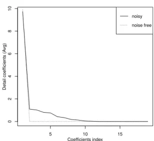
We use simulation to establish a simple proof of concept regarding compression by TGUH. Specifically, we look at the use of our TGUH transform to compress a ‘barbell’ type of network, i.e., a network with two fully connected components joined by a single link. We generated such a barbell with

10 nodes in each fully connected component and applied the TGUH transform described in Algorithm 1. All detail coefficients are zero except that resulting from the last step of the algorithm, where the two connected components merge together, which demonstrates that the TGUH transform is able to capture well the structure of the barbell network. The resulting compression curve is shown in Figure 1.

To demonstrate the robustness of this result, we simulated

100 such barbells perturbed with both Type I and Type II errors, i.e., declaring non-edges edges and vice versa. Here we set P(Type I error) = 0.01 and P(Type II error) = (1− Den)/Den×P(Type I error), where Den is the density of adjacency matrix of the noise-free barbell. Under this setting, the expected density of the ‘noisy’ network is the same as the original one. Figure1shows the average compression curve resulting from applying the TGUH to these noisy networks.

5 10 15 0 2 4 6 8 10 Coefficients index Detail coefficients (A vg) noisy noise free

Fig. 1: Compression curve for barbell network (dotted) and average compression curve for noisy barbell network (solid) using TGUH.

We see that this curve is qualitatively quite similar to that for the noise-free version of these networks.

B. EEG data on a DTI network

We now provide an application of using the TGUH to denoise EEG signals over a DTI network. Understanding the relationship between brain anatomical connectivity and brain dynamics remains an active research area [4] [17]. In general, different frequency bands have been associated with different brain function [2], and different spatial organization over the brain’s surface, but how brain anatomical connectivity relates to brain rhythms remains incompletely understood.

As an example application of the method developed here, we consider two types of data collected from a human subject. Brain anatomical connectivity was computed from high resolution diffusion tensor imaging data using previously described methods [4]. Briefly, 324 regions of interest (ROI) at the gray-white matter border were selected using the topology of a recursively subdivided icosahedron fitted in the subject’s cortical surface inflated to a sphere [9] [12]. Quantitative bidirectional white matter connectivity between each ROI pair was computed using Probtrackx2 software [1] where 500 streamlines were sampled per voxel within each ROI. A connectivity index was then computed for each ROI pair as the proportion of successful streamlines connected between the ROI pair over the total number of streamlines sampled.

Dynamic brain electrical activity was collected from the same ROIs using the MNE-C and Freesurfer software packages [9] [13] and previously reported methods [4]. Briefly, EEG data during stage 2 sleep was recorded with a 70 channel EEG cap and electrode positions collected using a 3D digitizer. Anatomical cortical surfaces of the brain were reconstructed

(6)

using T1-weighted MRI data and a forward solution was cal-culated using a three-layer boundary element model consisting of the inner skull, outer skull and outer skin surfaces. The digitized EEG electrode coordinates were coregistered to the reconstructed surface using the nasion and auricular points. The inverse operator was computed from the forward model and the resultant current estimates at each ROI calculated. Ten seconds of artifact free data were selected for analysis. From the electrical source estimates at each ROI, we computed the power spectrum using the multitaper method (bandwidth 1 Hz, 9 tapers). We then compute the average power in the theta band (5-8 Hz), alpha band (8-12 Hz), beta band (12-20 Hz), and gamma band (20-40 Hz).

The DTI network contains 324 nodes and 1487 edges. Power in each spectral band was compressed using the TGUH bases on the DTI network. The resulting compression curves appear in Figure2. In all four bands, half of the signals were captured using the leading 50basis functions.

0 50 100 150 200 250 300 0 200 400 600 x theta Coefficients retained Appro ximation error 0 50 100 150 200 250 300 0 200 400 600 800 x alpha Coefficients retained Appro ximation error 0 50 100 150 200 250 300 0 100 200 300 400 500 600 700 x beta Coefficients retained Appro ximation error 0 50 100 150 200 250 300 0 100 200 300 400 500 600 x gamma Coefficients retained Appro ximation error

Fig. 2: Compressed spectral bands of the TGUH bases To illustrate TGUH denoising, we only show the result of denoising the alpha band signal, in Figure 3. There the size of the nodes indicates the strength of the signal. Using the theoretical threshold suggested by Theorem III.1, signal on only 6 nodes in the occipital cortex remain; the rest has been eliminated. The intuition is that the cluster of electrodes with increased alpha power likely represents the posterior dominant rhythm in this area.

V. DISCUSSION& FUTURERESEARCH

In this paper, we develop a new class of graph wavelets, based on adaptive unbalanced Haar transformations, and

(a) Noisy signal (b) Denoised signal

Fig. 3: (a) alpha band of the DTI network; (b) denoised alpha band of the DTI network.

establish consistency for estimating appropriate functions over a network. Theoretical analysis, simulation, and real data application in the context of computational neuroscience suggest the promise of this class. Our algorithm is especially useful in the case where the signal behaves differently at different scales and these scales correspond to analogous variations in the underlying network topology.

Even with the current advancement in this now-highly-active space, the interaction of network topology, basis and signal is still an under-explored area. In future work, denoising of the network itself seems a natural extension here, although theo-retical analysis even in toy cases is challenging. Connections to graph coarsening and visualization are possible as well.

VI. ACKNOWLEDGEMENTS

We would like to thank Lauren M Ostrowski and Daniel Y Song for collecting and cleaning the DTI data. This work was supported in part by EPSRC grant no. EP/L014246/1, AFOSR award 12RSL042, and NIH award 1R01NS095369-01.

VII. PROOFS

A. Proof of Theorem III.1

Proof. The fact that P(A) → 1 as N → ∞ follows from Lemma 1 of [24]. We begin by defining two sets S`

0 and S1` with S1` =

1≤r≤k(`) :the support ofψ`_r crosses multiple regions of constancy at level`}andS0`={1,· · ·, k(`)}\S1`.

R( ˆf , f) = 1 N X v ( ˆf(v)−f(v))2 = 1 N L X `=1 k(`) X r=1 α`_rI ∃V`0 r0 ⊆V ` r |α`0 r0 |> λ(` 0_{, r}0₎ −µ`_r 2 + 1 N (α0₀−µ0_{0 )}2 = 1 N L X `=1     X r∈S`₀ + X r∈S`₁     α`_rI ∃V_r`0 ⊆0 V_r` |α`_r00 |> λ(`0, r0) −µ`_r 2 + 1 N (α0₀−µ0_{0 )}2 ≤ 1 N L X `=1     X r∈S`₀ + X r∈S`₁     α`_rI ∃V_r`0 ⊆0 V_r` |α`_r00 |> λ(`0, r0) −µ`_r 2 + 2 N logN

(7)

By Lemma VII.1, we have that on the set S` 0, |α`r|≤ √ 2 logN (q |Vm`0 −1|+ q |V`0 −1 m0 | q |Vm`0 −1|+|V` 0 −1 m0 | ) . We then have R( ˆf , f)≤ 1 N L X `=1 X r∈S`₁ α`_rI n ∃V_r`00⊆V_r` |α `0 r0|> λ(` 0 , r0)o−µ`_r2 + 2 NlogN .

Denote by E the event

       ∃V `0 r0 ⊆V `r |α`0 r0 |> √ 2 logN        q |Vm`0 −1|+ r |V`0 −1 m0 | q |V `_r|               . We compute (α`rI(E)−µ`r) 2_{= (}_α` rI(E)−α`r+α ` r−µ ` r) 2 ≤(α`_r)2I(¬E) + (α`r−µ ` r) 2_{+ 2}_|_α` rI(¬E)||α`r−µ ` r| ≤λ2+ 2λp2 logN+ 2 logN ≤(6 + 4√2) logN .

Note that the levelL associated with the TGUH transforma-tion is bounded, i.e., L ≤ logN/log(1−ρ)−1. Combining this with the fact that |S_`1|≤ K, and the assumption that

K = o N/log2N

, we have that R( ˆf , f) is of order O_NK_log(1−log2_ρN₎−1

. Lemma VII.1. Let S`

0 ={1≤m ≤k(`) :µ`r = 0}. On A, for `= 1,· · ·, L, k∈S` 0, we have |α`_r|≤p 2 logN      q |Vm`−1|+ q |V`−1 m0 | p |V` m|      .

Proof. Denote the two sub-regions which merge intoVr`in the next level asV`−1 m andV `−1 m0 . OnA, for`= 1,· · ·, L, k∈S`₀, we have α ` r = ( |V`−1 m0 | |V` r| )1/2P v∈Vm`−1(v) q |Vm`−1| − ( |V_m`−1| |V` r| )1/2P v∈V`−1 m0 (v) q |V`−1 m0 | ≤p 2 logN   ( |V_m`−01| |V` r| )1/2 + ( |V`−1 m | |V` r| )1/2  =p2 logN ( |V_m`−01|1/2+|Vm`−1| 1/2 |V` r|1/2 ) . REFERENCES

[1] T. E. Behrens, H. J. Berg, S. Jbabdi, M. F. Rushworth, and M. W. Woolrich, “Probabilistic diffusion tractography with multiple fibre orientations: What

can we gain?”Neuroimage, vol. 34, no. 1, pp. 144–155, 2007. [2] G. Buzsáki, “Rhythms of the Brain". Oxford University Press, 2006. [3] S. Chen, R. Varma, A. Singh, J. Kovaˇcevi´c, “Representations of piecewise

smooth signals on graphs”, Proceedings of the IEEE International Conference on Acoustics, Speech and Signal Processing, 6370–6374, 2016.

[4] C. J. Chu, N. Tanaka, J. Diaz, B. L. Edlow, O. Wu, M. Hämäläinen, S. Stufflebeam, S. S. Cash, and M. A. Kramer, “Eeg functional connectivity is partially predicted by underlying white matter connectivity,”Neuroimage, vol. 108, pp. 23–33, 2015.

[5] R. Coifman and W. Leeb, “Earth mover’s distance and equivalent metrics for spaces with hierarchical partition trees,” 2013.

[6] R. R. Coifman and M. Maggioni, “Diffusion wavelets,” Applied and Computational Harmonic Analysis, vol. 21, no. 1, pp. 53–94, 2006. [7] M. Crovella and E. Kolaczyk, “Graph wavelets for spatial traffic analysis,”

inINFOCOM 2003. Twenty-Second Annual Joint Conference of the IEEE Computer and Communications. IEEE Societies, vol. 3. IEEE, pp. 1848– 1857.

[8] P. Fryzlewicz, “Tail-greedy bottom-up data decompositions and fast multiple change-point detection,”Annals of Statistics, to appear, 2017. [9] B. Fischl, “Freesurfer,”Neuroimage, vol. 62, no. 2, pp. 774–781, 2012. [10] P. Fryzlewicz and C. Timmermans, “Shah: Shape-adaptive haar wavelets

for image processing,”Journal of Computational and Graphical Statistics, vol. 25, no. 3, pp. 879–898, 2016.

[11] M. Gavish, B. Nadler, and R. R. Coifman, “Multiscale wavelets on trees, graphs and high dimensional data: Theory and applications to semi supervised learning,” inProceedings of the 27th International Conference on Machine Learning (ICML-10), 2010, pp. 367–374.

[12] A. Gramfort, M. Luessi, E. Larson, D. A. Engemann, D. Strohmeier, C. Brodbeck, R. Goj, M. Jas, T. Brooks, L. Parkkonenet al., “Meg and eeg data analysis with mne-python,”Frontiers in neuroscience, vol. 7, 2013.

[13] M. S. Hamalainen and J. Sarvas, “Realistic conductivity geometry model of the human head for interpretation of neuromagnetic data,” IEEE transactions on biomedical engineering, vol. 36, no. 2, pp. 165–171, 1989.

[14] D. K. Hammond, P. Vandergheynst, and R. Gribonval, “Wavelets on graphs via spectral graph theory,”Applied and Computational Harmonic Analysis, vol. 30, no. 2, pp. 129–150, 2011.

[15] J. Irion and N. Saito, “Efficient approximation and denoising of graph signals using the multiscale basis dictionaries,”IEEE Transactions on Signal and Information Processing over Networks, 2017.

[16] E.D. Kolaczyk, “Statistical Analysis of Network Data: Methods and Models.” Springer New York, 2009.

[17] N. J. Kopell, H. J. Gritton, M. A. Whittington, and M. A. Kramer, “Beyond the connectome: the dynome,”Neuron, vol. 83, no. 6, pp. 1319– 1328, 2014.

[18] R. Kondor, N. Teneva, and V. Garg, “Multiresolution matrix factorization,” inProceedings of the 31st International Conference on Machine Learning (ICML-14), 2014, pp. 1620–1628.

[19] A. B. Lee, B. Nadler, and L. Wasserman, “Treelets: an adaptive multi-scale basis for sparse unordered data,”The Annals of Applied Statistics, pp. 435–471, 2008.

[20] F. Murtagh, “The haar wavelet transform of a dendrogram,”Journal of Classification, vol. 24, no. 1, pp. 3–32, 2007.

[21] A. Sandryhaila and J.M.F. Moura, “Discrete signal processing on graphs,”

IEEE Transactions on Signal Processing, vol. 61, no. 7, pp. 1644–1656, 2013.

[22] D. I. Shuman, S. K. Narang, P. Frossard, A. Ortega, and P. Vandergheynst, “The emerging field of signal processing on graphs: Extending high-dimensional data analysis to networks and other irregular domains,”IEEE Signal Processing Magazine, vol. 30, no. 3, pp. 83–98, 2013.

[23] A. Singh, R. Nowak, and R. Calderbank, “Detecting weak but hierarchically-structured patterns in networks”,Proceedings of the Thir-teenth International Conference on Artificial Intelligence and Statistics (AISTATS), 749–756, 2010.

[24] Y-C. Yao, “Estimating the number of change-points via Schwarz’criterion,"Statistics and Probability Letters, vol. 6, no. 3, pp. 181–189, 1988.