University of Pennsylvania
ScholarlyCommons
Statistics Papers Wharton Faculty Research
2011
VIF Regression: A Fast Regression Algorithm for
Large Data
Dongyu Lin
University of PennsylvaniaDean P. Foster
University of PennsylvaniaLyle H. Ungar
University of PennsylvaniaFollow this and additional works at:http://repository.upenn.edu/statistics_papers
Part of theApplied Statistics Commons
This paper is posted at ScholarlyCommons.http://repository.upenn.edu/statistics_papers/505
For more information, please [email protected].
Recommended Citation
Lin, D., Foster, D. P., & Ungar, L. H. (2011). VIF Regression: A Fast Regression Algorithm for Large Data.Journal of the American Statistical Association, 106(493), 232-247.http://dx.doi.org/10.1198/jasa.2011.tm10113
VIF Regression: A Fast Regression Algorithm for Large Data
AbstractWe propose a fast and accurate algorithm,VIF regression, for doing feature selection in large regression
problems. VIF regression is extremely fast: it uses a one-pass search over the predictors, and a computationally efficient method of testing each potential predictor for addition to the model. VIF regression provably avoids model over-fitting, controlling marginal False Discovery Rate (mFDR). Numerical results show that it is much faster than any other published algorithm for regression with feature selection, and is as accurate as the best of the slower algorithms.
Keywords
marginal false discovery rate, model selection, stepwise regression, variable selection Disciplines
VIF Regression:
A Fast Regression Algorithm For Large Data
Dongyu Lin, Dean P. Foster, and Lyle H. Ungar ∗
Abstract
We propose a fast and accurate algorithm,VIF regression, for doing feature selection in
large regression problems. VIF regression is extremely fast: it uses a one-pass search over the predictors, and a computationally efficient method of testing each potential predictor for addition to the model. VIF regression provably avoids model over-fitting, controlling marginal False Discovery Rate (mFDR). Numerical results show that it is much faster than any other published algorithm for regression with feature selection, and is as accurate as the best of the slower algorithms.
KEY WORDS: Variable selection; stepwise regression; model selection; marginal False Discovery Rate.
∗Dongyu Lin is Postdoctoral Fellow, Department of Biostatistics and Epidemiology, University of Pennsylvania
School of Medicine, Philadelphia, PA 19104 (E-mail: [email protected]). Dean P. Foster is Marie and
Joseph Melone Professor, Department of Statistics, The Wharton School, University of Pennsylvania,
Philadel-phia, PA 19104 (E-mail: [email protected]). Lyle H. Ungar is Associate Professor, Department of Computer and
Information Science, University of Pennsylvania, Philadelphia, PA 19104 (E-mail: [email protected]). The
authors thank Professor Lawrence D. Brown for sharing the call center data. The authors also thank the Editor,
1 INTRODUCTION
Datasets from areas including genetic sequences, text mining the web, image processing, and sen-sor networks can now easily have millions of observations and hundreds of thousands of features. Even a medium sized dataset can create a huge number of potential variables if interactions are considered. The problem of variable selection or feature selection, which aims to select the most predictive of an enormous number of candidate features, plays an increasingly important role in modern research (Guyon and Elisseeff 2003).
The specific problem that we consider here is how to improve the speed of variable selection algorithms for linear regression models of very large-scale data. Linear regression models are widely used for building models for large problems; their simplicity makes them fast and easy to evaluate.
The statistical embodiment of variable selection we consider here is a classic normal linear model
y=Xβ+ε, (1)
with n observationsy= (y1, . . . , yn)0 and ppredictorsx1, . . . ,xp,pn, whereX= (x1, . . . ,xp)
is an n×p design matrix of features, β = (β1, . . . , βp)0 is the vector of coefficient parameters,
and error ε ∼N(0, σ2In).
The number of the features in the dataset is often much larger than the number of the observations. In these cases, we need to either regularize the coefficient parameters β in (1), or select a subset of variables that can provide a jointly predictive model, assuming that only a subset of k of the p predictors {xj}pj=1 in (1) has nonzero coefficients (Miller 2002) . The paper presents a fast algorithm for searching for such a low dimensional model.
Our Variance Inflation Factor (VIF) regression algorithm has a computation complexity
O(pn) under the sparsity assumption that k p . This speed enables the VIF algorithm to handle larger data sets than many competitors, as illustrated in Figure1. The VIF regression
algorithm also guarantees good control of the marginal False Discovery Rate (mFDR) (Foster
and Stine 2008) with no over-fitting, and hence provides accurate predictions. Figure 2 shows
the out-of-sample performance of VIF and four competing algorithms. VIF regression is more accurate than its fastest competitor, GPS (Friedman 2008), and is of comparable accuracy to its slow but accurate competitors, such as stepwise regression.
[Figure 1 about here.]
[Figure 2 about here.]
1.1 Related Work
Variable selection algorithms are generally designed to seek an estimate of β that minimizes the
lq penalized sum of squared errors
arg minβky−Xβk2 2+λqkβklq , (2) where kβklq = ( Pp i=1|βi|q)1/q for q >0 and kβkl0 = Pp i=1I{βi6=0}.
The aforementioned problem of selecting a subset of variables corresponds to using anl0 norm in (2). This problem is NP hard (Natarajan 1995), yet its solution can be greedily approximated by stepwise regression, a standard statistical tool. Stepwise regression works well for moderate sized datasets, but has a relatively high computation complexity, O(np2q2). It can become very slow when n is large, since o(n/logn) variables can enter the model without over-fitting
(Greenshtein and Ritov 2004; Breiman and Freedman 1983). Zhang (2009) developed a new
optimization algorithm FoBa, which also addresses the l0 problem, and provides a theoretical bound on its accuracy. However, FoBa is extremely slow, as shown in our experiments; also, unlike VIF regression, it requires cross validation to decide the sparsity of the model.
A rich literature has been developed in recent years solving (2) using an l1 norm penalty. Exact solutions can be found efficiently due to the convexity of the l1 problem, for example, Lasso/LARS (Efron et al. 2004) and the Dantzig Selector (Candes and Tao 2007). These l1
methods have, however, several limitations. First, cross validation is required to determine the penalty λ1; this is time consuming and is not realizable in the setting where predictors are generated dynamically. Second, implementations of these algorithms have historically been slow. Our experiments (Section 6) show that Lasso is slow compared to other algorithms; the implementation of the Dantzig Selector is even slower than the quadratic algorithms (Hastie
et al. 2009) although it can be solved by linear programming. Faster algorithms in this category
include coordinate descent (Friedman et al. 2010) and GPS (Friedman 2008). We will show in Section 6that our algorithm is faster than the fastest of these algorithms, GPS.
More importantly, l1 algorithms lead to biased estimates (Candes and Tao 2007) and tend to include more spurious variables than l0 methods, and thus do not perform as well as greedy algorithms in highly sparse systems (Zhang 2009). This bias is due to the fact that these methods minimize a relaxed problem and hence achieve suboptimal solutions to the original problem (Lin
et al. 2008). As a result, these optimization algorithms have less accurate predictions; as shown
in Figure 10, models built by Lasso and GPS are not as accurate as the model fitted using our VIF regression algorithm.
Solving the non-convex problems efficiently is still highly challenging, but progress has been reported toward this goal (Friedman 2008). In the extreme non-convex case where an l0 penalty is applied, stepwise regression is still the most accurate approximation algorithm. The VIF regression algorithm we present in this paper is, in fact, an improved, much faster version of stepwise regression.
1.2 Our VIF Regression Approach
Our VIF algorithm is characterized by two components:
• The evaluation step, where we approximate the partial correlation of each candidate vari-able xi with the response variable y by correcting (using the “variance inflation factor”)
O(n) for each variable.
• The search step, where we test each variable sequentially using an α-investing rule (Foster
and Stine 2008). The α-investing rule guarantees no model over-fitting and provides highly
accurate models.
The evaluation step inherits the spirit of a variation of stepwise regression,forward stagewise regression, which evaluates variables only using marginal correlations. The small step-size for-ward stagewise regression algorithm behaves similarly tol1 algorithms, such as Lasso and LARS
(Efron et al. 2004); hence, like its siblings, it suffers from collinearities among the predictors and
will also introduce bias in the estimates. Herein, we correct this bias by pre-sampling a small set of data to compute thevariance inflation factor (VIF) of each variable. The resulting evaluation procedure is fast and does not lose significant accuracy.
This novel VIF procedure can be incorporated with a variety of algorithms, including stepwise regression, LARS and FoBa. As a demonstration, we incorporate this evaluating procedure with a streamwise regression algorithm using an α-investing rule to take full advantage of its speed. Streamwise regression (Zhou et al. 2006) is another variation of stepwise regression. It considers the case where predictive features are tested sequentially for addition to the model; since it considers each potential feature only once, it is extremely fast. The resulting VIF regression algorithm is especially useful when feature systems are dynamically generated and the size of the collection of candidate features is unknown or even infinite. It can also serve as an “online” algorithm in order to load extremely large-scale data into RAM feature by feature. (Note that our method is online in f eatures, unlike most online regression methods, which are online in observations.)
Our approach is statistics-based in the sense that we add variables only when they are able to pay the price of reducing a statistically sufficient variance in the predictive model. The “price”, or the penaltyλ0 in (1), is well studied in statistics. Classic criteria for the choices include Mallows’
approaches, our algorithm does not require cross validation.
We compare our VIF algorithm with classic stepwise regression, Lasso algorithm, and two recently developed algorithms: GPS (Friedman 2008) and FoBa (Zhang 2009). Our experiments give two main results: 1) the VIF regression algorithm is much faster than any other published algorithms; and 2) the VIF algorithm is comparably accurate to (the slow) stepwise regression and FoBa, but is more accurate than (the fast) GPS and Lasso.
The rest of the paper is organized as follows. In Section 2 we compare single steps in for-ward stepwise regression and forfor-ward stagewise regression and show that the coefficient estimate provided by the latter is biased by a factor caused by the multicollinearity and hence needs to be corrected. We propose and present the sped-up streamwise algorithm in Section 3, and note that our algorithm avoids overfitting; it controls the marginal False Discovery Rate (mFDR). In Section 4, the choice of subsample size, which decides the speed of the algorithm, is discussed. Section 5 provides guarantees against underfitting, proving that needed high signal predictors will not be missed. Finally, we experimentally compare VIF against competing methods on several data sets in Sections 6 and 7.
2 FORWARD SELECTION AND BIAS CORRECTION
2.1 Forward Feature Selection
Optimally solving (2) with an l0 penalty requires searching over all 2p possible subsets, which is NP hard (Natarajan 1995), and hence computationally expensive even whenpis small. Compu-tationally tractable selection procedures have been designed to overcome this problem in light of the model sparsity and the fact that a majority of the subset models can be ignored. Stepwise regression is such an algorithm.
Stepwise regression sequentially searches for predictors that collectively have strong predic-tivity. In each step, a multivariate model is statistically analyzed, and a new variable may be added in, or an existing variable may be removed from the current model. Common procedures
include forward selection, backward elimination, and forward-backward combination. Forward selection starts from a constant term1nand adds one predictor at a time; backward elimination
starts from the full set of predictors and removes one predictor in each step. Both have their own advantages and disadvantages. For data mining applications, however, backward algorithms are unrealistic because of the computational complexity of building models with enormous number of potential explanatory variables. In contrast, forward procedures are much faster, and thus more desirable.
Since a multiple regression is needed foreach candidate predictor in forward stepwise regres-sion, O(npq2) computation is required foreach step, whereq is the number of variables included in the current model. We assume p n. Given the vast set of potential predictors involved, substantial CPU time is often required. Hence, constructing a more efficient algorithm that can reduce the computational complexity is attractive.
In contrast, in forward stagewise regression, only marginal estimates, but not partial esti-mates, will be computed in each evaluation step. Therefore, onlyO(np) computation is needed, and it is much faster than forward stepwise regression.
We now show that forward stagewise regression leads to a bias which must be corrected to get optimal performance. The correction of this bias with be the core of our Variance Inflation Factor method.
2.2 Bias Correction
To show that the stagewise evaluation procedure is biased, consider a scheme in whichkpredictors have already been added to the model, and we are searching for the k+ 1st predictor. Without loss of generality, assume that all the predictors are centered and normalized. Since our goal is to find a collectively predictive linear model, the alternative hypothetical model that we want to test is
y=β0+β1x1+· · ·+βkxk+βnewxnew+ε,ε ∼N(0, σ2I). (3)
where1n,x1, . . . ,xk are linearly independent variables. We abuse the notation and remain using
σ2 to denote the variance of the errors. Note that this σ2 might be different from the more general one in Section 1. Denote X = [1n x1 · · · xk], ˜X = [X xnew], β = (β0, . . . , βk)0 and
˜
β = (β0, . . . , βk, βnew)0.
Let ˆβnewbe the least squares estimate of βnewin model (3). Letrbe the residual of projecting
y on{1n} ∪ {xi}ki=1. The hypothetical model being considered in stagewise regression is
r =γnewxnew+ ˜ε, ε˜∼N(0,σ˜2I). (4)
We let ˆγnew be the least squares estimate of γnew in this model (4) and have the following proposition:
Proposition 1. Under model (3),
ˆ
γnew =ρ2βˆnew, (5)
where
ρ2 = x0new(I−X(X0X)−1X0)xnew (6)
= hxnew,P⊥Xxnewi=hP⊥Xxnew,P⊥Xxnewi
andP⊥X is the projection onto the orthogonal complement of the hyperplane spanned by{1n,x1, . . . ,xk}, in the space spanned by {1n,x1, . . . ,xk,xnew}.
Proof. First note that
˜ X0X˜ = X0X X0xnew
x0newX x0newxnew
,
( ˜X0X˜)−1 = ∗ ∗∗ −ρ−2x0 newX(X 0X)−1 ρ−2 , (7) where ∗= (X0X)−1+ρ−2(X0X)−1X0xnewx0newX(X 0 X)−1 and ∗∗=−ρ−2(X0X)−1X0xnew. Hence,
ˆ βnew = ( ˜X0X˜)−new1 X˜ 0 y = −ρ−2x0newX(X0X)−1X0y+ρ−2x0newy = ρ−2x0newr=ρ−2ˆγnew.
A simple case with two variables, shown in Figure 3, illustrates the underlying geometric mechanism of Proposition 1.
[Figure 3 about here.]
Proposition1suggests that the stagewise coefficient estimate ˆγnew is simply a scaled stepwise coefficient estimate ˆβnew. Thus, if the predictors are all centered, both of the hypothesis tests,
H0 : βnew = 0 and H0 : γnew = 0, can detect whether or not xnew contributes to the model. However, the amount of the contribution that is detected by these two tests is fundamentally different.
Under model (3), the expected estimated variance of ˆβnew is
E \ Var( ˆβnew) =Eh( ˜X0X˜)new−1 σˆ2stepi =ρ−2σ2 by (7), where ˆσ2 step = (krk2−ρ −2(x0
newr)2)/(n−k−2) is the mean squared error of this model. On the other hand, under model assumption (4),
EhVar(ˆ\γnew) i
where ˆσ2
stage = (krk2−(x
0
newr)2)/(n−1) is the mean squared error of model (4). Therefore, we have approximately
\
Var(ˆγnew)≈ρ2Var( ˆ\βnew). (8)
It follows that the corresponding t-ratios satisfy
t(stagewise)new ≈ |ρ| ·t(stepwise)new (9)
The simulation result in Figure 4 demonstrates that these two t-ratios differ by a factor of approximately ρ.
[Figure 4 about here.]
This bias is caused by the misspecified model assumption: under model (3), model (4) is not valid. If ρ2 = 1, x
new is orthogonal to X, and these two procedures are identical; however, if
ρ2 <1, or x
new is correlated with X, the errors in model (4) should be correlated. In the latter case, the common model hypothesis testing, which assumes error independence, will not lead to a correct conclusion.
To some extent, forward stepwise regression provides a more powerful procedure in the sense that predictors that can be detected by stagewise regression will be spotted by stepwise regression as well, but not necessarily vice versa. In contrast, the forward stagewise procedures may prefer a spurious predictor that is less correlated withXto an indeed predictable variable that is highly correlated with X. One of the criticisms of forward selections is that they can never correct the mistakes in earlier steps (Zhang 2009); the inclusion of this spurious variable in the model might lead to more bias. If the data have strong multicollinearity, the stagewise algorithm will reach a resulting model that is not so predictive.
In order to illustrate this fact, we simulatedp= 200 features whose are jointly Gaussian and their covariance matrix has a form as (17) withθ = 0.9 and τ2 = 0.1; the way we simulated the response variable y is similar to the simulations in Section 6.3. We compared two algorithms:
the VIF regression algorithm we propose in Section 3, and a Na¨ıve algorithm which is exactly the same as the VIF regression algorithm except that it does not have the t-statisticcorrection
procedure.
[Figure 5 about here.]
Over 50 replications, we found that on average VIF regression chose 91% of the true variables, while the na¨ıve algorithm chose 47.3% of the true ones. Figure5showed the out-of-sample error rate of these two algorithms and Lasso on the same sets of data. It is obvious that the na¨ıve algorithm without a correction procedure does not perform as well as an algorithm based on the corrected statistics.
2.3 The Fast Evaluation Procedure
In order to speed up the evaluation procedure, we take advantage of the economical computation of forward stagewise regression, but correct the biased t-ratio in each step, thus giving results similar in accuracy to the stepwise regression procedures.
To this end, we need to estimate the true sample distribution of ˆγnew under model (3):
Proposition 2. Under model assumption (3),
ˆ
γnew ∼N ρ2βnew, ρ2σ2
. (10)
Proof. Since by (7), ˆβnew ∼N(βnew, ρ−2σ2), it follows by Proposition 1.
Now that ˆγnew/(|ρ|σ) ∼ N(0,1), with proper estimates of ρ and σ, we can have an honest
t-ratio for testing whether or not βnew= 0:
• σˆ can be estimated by the root mean square error ˆσnull under the null modelH0 :βnew= 0. Unlike ˆσstep or ˆσstage (Section2.2), which are the common estimated standard deviations in regression analysis, the use of this null estimate ˆσnull can avoid over-fitting or introducing selection bias, especially in data with heteroskedasticity (Foster and Stine 2004).
• ρˆ: ρ can be calculated precisely by proceeding with a multiple regression of xnew on
C = {1n,x1, . . . ,xk}, then computing ρ2 = 1−R2new|1···k, the unexplained proportion of
variation. This computation, however, is as expensive as the stepwise procedure, and thus not desirable. Unfortunately, there is no easy way to estimateρbecause of the dependence issue we discussed earlier. Most tools, including the bootstrap, break down because of dependency among the errors, which are the only numerical products after performing a stagewise regression. Our solution to this is to randomly sample a size m subset of the whole dataset and use this subset to estimateρ2 in light of the fact thateach random subset should represent the whole data. We will discuss the choice of m in Section 4.
Our fast evaluation procedure is summarized below:
The Fast Evaluation Procedure
At each step of the regression, suppose a set of predictorsC ={x1, . . . ,xk}have been chosen
in the model. We assume below that all the variables xi are centered.
1. Obtain residualsr=y−XC(X0CXC)−1X0Cyand root mean square error ˆσnull=krk/ p
(n− |C| −1) from the previous step;
2. Sample a small subset I = {i1, . . . , im} ⊂ {1, . . . , n} of observations; let xI denote the
corresponding subsample of predictors x;
3. Fitr on xnew/kxnewk and compute the coefficient estimate ˆγnew =hr,xnewi/kxnewk; 4. FitxInew on {xI1, . . . ,xIk}and compute R2I =x0newXIC (XIC)0XIC−1(XIC)0xnew/kxnewk2;
5. Compute and return the approximate t-ratio as ˆtnew= ˆγnew/(ˆσ p
1−R2
I).
3 VIF REGRESSION
The fast evaluation procedure can be adapted to speed up a variety of stepwise-like algorithms, but it is most beneficial in massive data settings. Therefore, we incorporate it into a streamwise
variable selection algorithm using an α-investing rule.
3.1 α-investing, Sequential Testing and mFDR
An α-investing rule is an adaptive, sequential procedure for testing multiple hypotheses (Foster
and Stine 2008). The rule works as follows. Suppose this is a game with a series of tests. A
gambler begins his game with initial wealthw0; intuitively, this is an allowance for type I error. In theith test (game), at levelαi, if a rejection is made, the gambler earns apay-out∆w; otherwise,
his current wealthwi will be reduced by αi/(1−αi). The test levelαi is set to bewi/(1 +i−f),
where f is the time when the last hypothesis was rejected. Hence, once the gambler successfully rejects a null hypothesis, he earns more to spend the next few times. Furthermore, the game becomes easier to play in the near future in the sense thatαi will keep being inflated in the short
term. The game continues until the player goes bankrupt, i.e., wi ≤0.
Theα-investing rule naturally implements a Bonferroni rule, but overcomes its conservativity, controlling instead the marginal False Discovery Rate (mFDR).
False Discovery Rate(FDR) aims to control the Family-Wise Error Rate (FWER), arising in multiple statistical inferences (Benjamini and Hochberg 1995). In multiple hypothesis testing, successfully rejecting a null hypothesis is called a discovery. The classic definition of FDR is the expected proportion of false discoveries among all discoveries throughout the whole process,
FDR = E V R R > 0 P(R >0), (11)
whereV is the number of false positives, andRis the number of total discoveries. A few variants of FDR have been introduced in the past decade, including the marginal False Discovery Rate
(mFDR), which is defined asE(V)/E(R) orE(V)/(E(R) + 1); thepositive False Discovery Rate
(pFDR) (Storey 2002), which drops the termP(R >0) in (11); and thelocal false discovery rate
(fdr) (Efron et al. 2001), which is decided by the size of the test statistic z.
Proposition 3. An α-investing rule with initial alpha-wealth w0 ≤ αη and pay-out ∆w ≤ α
controls mF DRη =E(V)/(E(R) +η) at level α.
See Foster and Stine (2008) for the technical details of this theorem.
3.2 Steamwise Variable Selection and VIF Regression
Employing anα-investing rule allows us to test an infinite stream of hypotheses, while at the same time to control mFDR. In the context of variable selection, this implies that we may order the variables in a sequence (possibly dynamically) and include them into the model in a streamwise manner without over-fitting.
Over-fitting is a common problem in regression analysis. The model R2 will increase when a new variable is added, regardless of whether it is spurious or not. This in-sample over-fitting may result in terrible predictions when the model is used out of sample. Hence, the goal of all variable selection problems is to find a parsimonious model that has a satisfactory R2 or model fit in order to avoid over-fitting. These problems will typically impose a penalty on the number of variables in the model, namely, the l0 norm of the coefficient parameters, as we have introduced in Section1. Forward selections approach the solutions to these problems by properly thresholding the t-ratios of upcoming variables to control the number of the selected variables.
Being able to test the variables in a streamwise way has many advantages. First, the one-pass algorithm can save a great amount of computation if the data is massive. In most search algorithms, adding each new variable necessitates going through the whole space of candidate variables; the computation is expensive if the data size n×p is huge. We alleviate this burden by reducing the loops to only one round. Second, this allows one to handle dynamic variable sets. These include the cases where p is extremely large or unknown, resulting in a problem in applying static variable selection criteria. This also allows one to first test the lower order interactions and then decide which higher order interactions need testing.
in a streamwise way with a guarantee of no over-fitting. We state our VIF regression procedures in Algorithm1. We call it “VIF” because the correction factorρ in the key speed-up part is the
Variance Inflation Factor of the new variable with respect to the included variables. Algorithm 1 VIF Regression: the boosted Streamwise Regression using α-investing
Input: data y, x1,x2, . . . (centered);
Set: initial wealth w0 = 0.50 and pay-out ∆w= 0.05, and subsample size m;
Initialize C ={0}; r=y−y¯; ˆσ =sd(y);i= 1; w1 =w0; f = 0.
SampleI ={i1, . . . , im} ⊂ {1, . . . , n}.
repeat
set threshold αi =wi/(1 +i−f)
attain tˆi from theFast Evaluation Procedure // compute corrected t-statistic
if 2Φ(|ti|)>1−αi // comparep-value to threshold then
C =C ∪ {i} // add feature to model
update r=y−yˆC, ˆσ = RMSEC wi+1 =wi+ ∆w f =i else wi+1 =wi−αi/(1−αi) end if i=i+ 1
until maximum CPU time or Memory is reached * Φ is the CDF of the normal distribution.
One might worry that only going through the candidate predictors once may miss signal. In the worst case, it may in fact miss useful predictors. However, this will not happen in cases where the variables are orthogonal as in, for example, orthogonally designed experiments and signal processing (using a Fourier transform or wavelet transform); this also applies to distributionally orthogonal variables as in, for example, independent Gaussian entries in image processing. If predictors are highly correlated, each of these variables may contribute to the model since we are looking for a collectively linear model; as proven below, using an α-investing rule in this case guarantees that the final model will have certain predictability. Our experiments (Section
with those chosen by the most accurate algorithms for linear models. Furthermore, if we have prior knowledge of the predictors, for instance, for PCA variables, we can assign a higher priority to important variables so that they can get in the model more easily.
4 ACCURACY AND COMPUTATIONAL COMPLEXITY
Obviously, a large m (many observations used to test for inclusion of a feature) can guarantee an accurate approximation in our algorithm (Algorithm 1), but a small m will give faster com-putation. How large should m be in order to attain a reasonably accurate result? Ideally, we want to pick mn and small α and , such that
P |ˆρ| − |ρ| |ρ| ≤ ρ ≥1−α,
whereρis defined as in (6), the correlation betweenxnewand the perpendicular space of the space spanned by included variables; ˆρis the sample correlation betweenxInewand span{1m,xI1, . . . ,xIk}⊥.
This implies that with high probability, the bias in the correlation due to the sub-sampling is not large compared with the true correlation. Then roughly with probability at least 1−α, the approximate t-ratio is:
|tˆ| = |ˆγnew| ˆ σ|ρˆ| = |ˆγnew| ˆ σ|ρ|1 + |ρˆ|−||ρ|ρ| ≈ |ˆγnew| ˆ σ|ρ| 1− |ˆρ| − |ρ| |ρ| .
Consequently, with probability at least 1−α,
(1−)|ttrue|/|tˆ|/(1 +)|ttrue|. (12)
Recall thatρ2 = 1−R2new|1···k. Letz= P⊥Xxnew, where the operator P⊥X is defined as in
Propo-sition 1. Then ρ is the sample correlation of xnew and z. Assume furthermore that (xnew,z) are randomi.i.d. samples from a bivariate normal population with correlation ρ0, then
approxi-mately, 1 2log 1 +ρ 1−ρ approx ∼ N 1 2log 1 +ρ0 1−ρ0 , 1 n−3 .
Hence, conditional on the observations (and due to the fact that we sample without replace-ment), we have approximately:
1 2log 1 + ˆρ 1−ρˆ ρapprox∼ N 1 2log 1 +ρ 1−ρ , 1 m−3 . (13)
Since we focus on datasets with hugen’s and in high dimensional spaces, it is unlikely that two random vectors would be highly correlated. In fact, one can show that ad-dimensional space can tolerate up to O(d2) random vectors that have angles greater than π/4. In light of this fact and the approximate sample distribution (13), a crude calculation by assuming|ρ|>√2/2 shows that m ≥200 can guarantee an ≤0.1 and an α≤0.05 in (12).
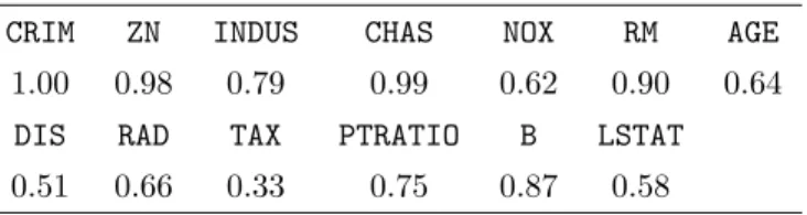
As a particular numerical example, we examined the Boston Housing data, which contains 506 census tracts in Boston from the 1970 census. This data and the data description can be downloaded from the UCI Repository of Machine Learning Databases at http://archive. ics.uci.edu/ml/. We took MEDV, the median value of owner occupied homes as our response variable. Serving as explanatory variables, the other thirteen variables were sequentially added in a multiple linear regression model. In each step, we computed the “true” t-ratio ttrue of the incoming variable by replacing the new RMSE with the old one (see Section 2.3). In addition, sub-sampling with size m = 200 and our fast evaluation procedure were repeated 100 times, resulting in a hundred fast t-ratios |˜t|. We then collected the ratios |˜t|/|ttrue|.
Figure6displays a comparative boxplot summarizing these experimental results on the thir-teen explanatory variables of the Boston Housing data. As shown in the boxplot, taking = 0.1, most of the ratios lie within the interval [1−,1 +]. To see how sensitive these bounds are to the actual correlation, we computed |ρ| based on Proposition 1; these |ρ|’s are annotated under the corresponding variables in Figure 6and are also listed in Table 8. Several variables have |ρ|
less than √2/2. For these variables, despite high variances, the ratios of absolute t-ratios are well bounded by 1±15%. This experiment validates our earlier claim that with a subsample size of m = 200, our fast evaluation mechanism can provide a tight bound on the accuracy in terms of the t-ratio approximation.
[Figure 6 about here.]
[Table 1 about here.]
Because VIF regression does a single pass over the predictors, it has a total computational complexity of O(pmq2), where m is the subsample size and q is the number of variables in the final model. Assuming sparsity in the model found, q can be much smaller than n; hence, as long as m = O(n/q2), which can be easily achieved based on our earlier discussion, the total computational complexity is O(pn).
5 STABILITY
Proposition3guarantees that our algorithm will not over-fit the data. In this section we develop a theoretical framework and show that our algorithm will not miss important signals.
A locally important variable gets added into the model if its reduction to the sum of squared errors exceeds the penalty λ that it brings to the penalized likelihood. However, if this impor-tance can be washed out or masked by other variables, then for prediction purposes, there is no difference between this variable and its surrogates, thus neither of them can be claimed “true”. This situation is common in our application since we consider predictors that are correlated, or even highly correlated by including high-order interactions. One will lose predictive accuracy only when those globally important variables, which stand out in any scenarios, are missed. To this end, we propose the following theorem, which guarantees that none of these important variables will be missed.
LetMbe the subset of non-constant variables that are currently chosen. We define Sλ,η(M) = x: SSEM−SSEM∪x SSEM/(n− |M| −1) >(1 +η)λ (14)
as the collection of variables that are λ-important with respect to model Mand
Sλ,η =∩MSλ,η(M) (15)
as the collection of λ-important variables. Notice that both of these are random sets, in other words they depend on the observed data. Let ˆCstep, ˆCstream, and ˆCVIF be the models chosen by stepwise regression, streamwise regression with α-investing rule, and VIF-regression. An investing rule is called η-patient if it spends at a slow enough rate that it has enough saved to spend at least i−(1+η) on the ith variable. For example, both the investing rules in Zhou
et al. (2006) and Foster and Stine (2008) can be chosen to be η-patient. We have the following
theorem:
Theorem 1. When the algorithms stop, (1) Sλ,0 ⊂Cˆstep;
(2) If the number of candidate predictors p > 7 and an η-patient investing rule is used, then
S2 logp,η ⊂Cˆstream;
(3) Suppose that x’s are multivariate Gaussian. If we use an η(1−η)/2-patient investing rule and our sampling size mis large enough, then for any x∈S2 logp,η, we haveP(x∈CˆVIF)> 1−O(1/m).
In other words, any 2 logp-important variable will likely be included by the VIF-algorithm.
Proof. (1)∀x∈Sλ,η, ifx∈/ Cˆstep, thenSSECˆstep+|
ˆ
Cstep|·λσˆC2ˆstep < SSECˆstep∪x+(|
ˆ
Cstep|+1)·λσˆ2Cˆstep,
andSSECˆstep−SSECˆstep∪x < λσˆ
2 ˆ
Cstep =λSSECˆstep/(n−|
ˆ
Cstep|−1), which contradicts the definition of Sλ,η.
(2) Suppose that the current model is M0. If the next predictor xi ∈ S2 logp,η, then it has
t-statisticti that meets
P(|Z|>|ti|)< P
|Z|>p(1 +η)2 logp< 2 exp{−(1 +p η)2 logp/2}
(1 +η)2 logp <
1
p(1+η)
as long as p > 7. Hencex will be chosen by any η-patient investing rule.
(3) We follow the notation in Section 4. Suppose that the current model is M0. Let ρ = q
1−R2
xi|M0 >0 and ˆρ be its VIF-surrogate. If the next candidate predictorxi ∈ S2 logp,η has
VIF-corrected t-statistic ˆti and true t-statisticti, we have
P |tˆi|> s 1 + η 2 − η2 2 2 logp X,y,M0 ! > P |ˆti|>|ti| r 1− η 2 X,y,M0 = P |ρˆ|< p |ρ| 1−η/2 ρ ! =P ˆ ρ2 < ρ 2 1−η/2 ρ > Pρˆ2 < ρ21 + η 2 ρ > 1−m˜−1/28(1−ρ 2) +η 2ηρ φ(κ) + ˜m −1/23ρ2−1 2ρ κ 2φ(κ) + ˜m−1 1 2ρ2 −2 + 13 4 ρ 2 κ3φ(κ) −m˜−1(3ρ 2−1)2 8ρ2 κ 5 φ(κ) +O( ˜m−3/2). > 1−O(m−1), (16)
where ˜m = m −3/2 +ρ2/4, κ = ˜m1/2ηρ/4(1 −ρ2), φ(·) is the density function of standard normal distribution, and the expansion in the third line followed Konishi (1978), with m >
16(1−ρ2)/ρ2η2+ 2. Note that κ3φ(κ) is bounded, and the first two non-constant terms are as small as order m−1 with sufficiently large m; the third term is always positive which covers the last two terms. From these the final bound follows.
There have been several recent papers on the selection consistency of forward selection. Wang
(2009) used stepwise regression to screen variables and then performed the common l1 methods on the screened variables. The author showed that the screening path would include the true subset asymptotically and thus the consistency ofl1 methods might be pertained. Cai and Wang (2010) used orthogonal matching pursuit, which is essentially a stagewise regression algorithm. They showed that with certain stopping rules, the important variables (with large true β) can
be fully recovered with high probabilities. However, both papers assume near orthogonality and utilize parameters to constraint multicollinearity, with bounded eigenvalues in the former and mutual incoherence in the latter. Zhang (2009) has similar assumptions. In our statistical applications, however, multicollinearity is common since we consider interaction terms, and so such consistency results are of limited utility. Also, as long as multicollinearity exists, there is no proper definition for “true variables” since the significance of one variable might be washed out by other variables. Thus, the best one can achieve are theorems such as the one presented above guaranteeing that one will not miss high signal predictors if there are not other predictors highly correlated with them. If multiple predictors are high signal, but correlated, we will find at least one of them.
6 NUMERICAL EXPERIMENTS
To test the performance of VIF regression, we compare it with the following four algorithms: • ClassicStepwise Regression. For the penalty criterion, we use either BIC or RIC, depending
on the size of the data;
• Lasso, the classic l1 regularized variable selection method (Tibshirani 1996). Lasso can be realized by the Least Angle Regression (LARS) algorithm (Efron et al. 2004), scaling in quadratic time in the size,n of the data set.
• FoBa, an adaptive forward-backward greedy algorithm focusing on linear models (Zhang 2009). FoBa does a forward-backward search; in each step, it adds the most correlated predictor and/or removes the least correlated predictor. This search method is very similar to stagewise regression except that it behaves adaptively in backward steps. In Zhang
(2009), the author also provides a theoretical bound on the parameter estimation error. • GPS, the generalized path seeking algorithm (Friedman 2008). GPS is a fast algorithm
be as fast as linear in n (Friedman 2008). GPS can compute models for a wide variety of penalties. It selects the penalty via cross validation.
In the following subsections, we examine different aspects of these algorithms, including speed and performance, on both synthetic and real datasets. All of the implementations were in R, a widely-used statistical software package which can be found at http://www.r-project.org/. We emphasize that unlike our VIF algorithm and stepwise regression, whose penalties are chosen statistically, the other three algorithms are cast as optimization problems, and thus require cross validation to decide either the penalty function (GPS) or the sparsity (Lasso and FoBa). Since sparsity is generally unknown, to fairly compare these algorithms, we did not specify the sparsity even for synthetic data. Instead, we used 5-fold cross validation for Lasso and GPS and 2-fold cross validation for FoBa. Note that this only adds a constant factor to the computational complexity of these algorithms.
6.1 Design of the Simulations
In each simulation study, we simulated p features, x1, . . . ,xp. We mainly considered three cases
of collinearities: (1) x0s are independent random vectors with each Xij (the jth element of xi)
simulated from N(0,0.1); in other words, x’s are jointly Gaussian with a covariance matrix Σ1 =τ2Ip, whereτ2 ≡0.1; (2) x’s are jointly Gaussian with a covariance matrix
Σ2 =τ2 1 θ · · · θp−1 θ 1 · · · θp−2 .. . ... . .. ... θp−1 θp−2 · · · 1 (17)
with τ2 ≡0.1; and (3) x’s are jointly Gaussian with a covariance matrix Σ3 =τ2 1 θ · · · θ θ 1 · · · θ .. . ... . .. ... θ θ · · · 1 (18)
withτ2 ≡0.1. We randomly pickedq= 6 variables from thesepvariables. The response variable
y was generated as a linear combination of theseq variables plus a random normal noise. The q
predictors has equal weightsβ = 1 in the all subsection except Section6.5, where the weights are set to be {6,5,4,3,2,1}. The random normal noise in most subsections has mean 0 and variance 1 without further explanation; its variances varies from 0.4 to 4 in Section 6.5 to investigate different signal to noise ratios.
In all simulations, we simulated 2n independent samples, then used n of them for variable selection and another n for out-of-sample performance testing. The out-of-sample performance was evaluated using mean sum of squared errors: P2n
i=n+1(yi−xiβˆ)2/n, where ˆβ is the output
coefficient determined by the five algorithms based on the training set, namely the firstnsamples. The sample size n is fixed at 1,000 without further clarification. Since the true predictors were known, we also compared the true discovery rate and false discovery rate in Section 6.3.
6.2 Comparison of Computation Speed
We simulated the independent case to measure the speed of these five algorithms. The response variable y was generated by summing six of these features with equal weights plus a random noise N(0,1). Considering the speed of these five algorithms, the number of features p varies from 10 to 1,000 for all five algorithms, and from 1,000 to 10,000 for VIF Regression and GPS.
[Figure 7 about here.]
As shown in Figure7, VIF Regression and GPS perform almost linearly, and are much faster than the other three algorithms. Given the fact that it does a marginal search, the FoBa algorithm
is surprisingly slow; hence, we did not perform cross validation for this speed benchmarking.
[Figure 8 about here.]
To further compare VIF and GPS, Figure8 shows two close-up plots of the running time of these two algorithms. Both of them appear to be linear inp, the number of candidate predictors. Although GPS leads when p is small, VIF Regression has a smaller slope and is much faster when p is large.
6.3 mFDR Control
In order to test whether or not these algorithms successfully control mFDR, we studied the performance of the models chosen by these five algorithms based on the training set. We took the simulation scheme in Section 6.1 and the same simulation was repeated 50 times. We then computed the average numbers of false discoveries and true discoveries of features, denoted by
\
E(V) and E[(S), respectively. Taking an initial wealthw0 = 0.5 and a pay-out ∆w= 0.05 in our VIF algorithm, with an η = 10 in Proposition 3, the estimated mFDR is given by
\ mFDRη = \ E(V) \ E(V) +E[(S) +η . (19)
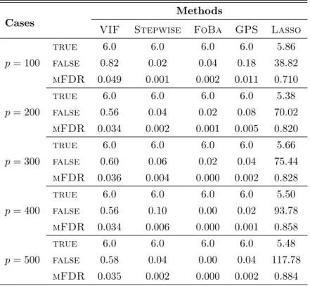
Summarized in Table 2are E[(S), the average number of true discoveries, \E(V), the average number of false discoveries, and mFDR\η, the estimated mFDR in the first simulation with
independent Gaussian features. As can be seen, with the exception of Lasso, the other four algorithms successfully spotted the six true variables and controlled mFDR well. This is not surprising, however, since these algorithms aim to solve non-convex problems (Section 1). Lasso solves a relaxed convex problem; hence, it tends to include many spurious variables and then shrinks the coefficients to reduce the prediction risk.
[Table 2 about here.]
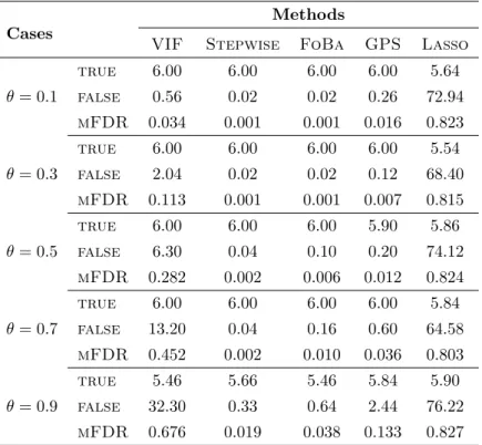
Table 3 provides a similar summary for the case where the features were generated using a multivariate Gaussian distribution with the covariance matrix given in (17). Lasso was again not able to control mFDR; both stepwise regression and FoBa controlled mFDR at low levels in all cases. GPS and VIF regression also did well except for the case with very high multicollinearity. However, as we mentioned earlier, in the case with high multicollinearity, each of the collinear predictors could make a contribution to the model accuracy, since we are building a nested model. Hence, it is hard to claim that the “false discoveries” are indeed false in building a multiple linear model. In any case, since our main purpose in employing an α-investing control rule is to avoid model over-fitting, we will look at their out-of-sample performance in the next subsection.
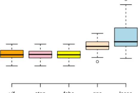
6.4 Out-of-sample performance
We used the aforementioned n = 1,000 held-out observations to test the models chosen by the five algorithms. The case with independently generated features is shown in Figure 9, which illustrates a comparative boxplot for the out-of-sample mean squared errors of the five chosen models in 50 runs. As can be seen, the models chosen by VIF regression perform as well as the two best algorithms, stepwise regression and FoBa, and does better than GPS and Lasso. Figure 10 provides a similar scenario for jointly Gaussian features, except for the case with extremely high correlation; VIF regression has slightly higher mean squared errors, but is still better than GPS and Lasso. The latter boxplot clarifies our claim that although more “false discoveries” were discovered by VIF regression, these features are not truly false. In fact, they helped to build a multiple model that did not overfit as demonstrated in Figure10. In this sense, VIF regression does control mFDR. Given the fact that VIF Regression is substantially faster than other algorithms, these results are very satisfactory.
[Figure 9 about here.]
6.5 The Effect of Signal-to-noise Ratio
To show how the signal-to-noise ratio may affect our algorithm, we took the simulation scheme with Σ2 and θ = 0.5 or 0.9. The number of features p was fixed to be 200. y was a linear combination of q = 6 random chosen variables, with weights from 1 to 6 plus an independent random noise N(0, ν2) where ν varies from 0.4 to 4. We used w0 = 0.5 and ∆w = 0.05 for the VIF algorithm.
We computed the out-of-sample mean squared errors on the n = 1,000 held-out samples. To provide a better illustration of the performance of the five algorithms, we report the ratio of the out-of-sample mean squared errors of other algorithms to that of VIF regression, i.e., P2n
i=n+1(yi − Xβˆother)2/ P2n
i=n+1(yi − Xβˆvif)2. A ratio less than (greater than) one implies a better (worse) performance of the algorithm compared to that of the VIF regression.
In general, VIF regression was slightly worse than stepwise regression and FoBa, but was much better than GPS and Lasso. When the multicollinearity of the variables was weak (with
θ = 0.5), as shown in Figure 11, the VIF regression had almost as well performance as stepwise regression and FoBa had (ratios were very close to one); GPS performed poorly when the signal is strong but approached closer to VIF when the signal got weaker; Lasso was consistently worse than VIF. When the multicollinearity of the variables was moderate (with θ = 0.9), Figure 12
shows that stepwise regression and FoBa could have more than 5% gain over the VIF regression; the performance of Lasso remained the same, but the performance of GPS was almost identical to that of VIF regression when the signal was weak. Thus, GPS benefited substantially from its shrinkage in cases when the noise was large and the multicollinearity was strong. In a nutshell, the VIF regression maintains its good performance under changing signal-to-noise ratios.
[Figure 11 about here.]
[Figure 12 about here.]
Fig-ure 13. Its performance was identical to that of VIF regression when θ= 0.5. This performance under weak multicollinearity was guaranteed in the literature (See, e.g., Tropp 2004; Cai and
Wang 2010). However, when the multicollinearity was moderate (θ = 0.9), the Na¨ıve algorithm
was worse than the one with VIF-correction, especially when the signal was relative strong. These results again demonstrate the necessity of the VIF-correction in real applications, where testing the mutual incoherence (weak multicollinearity) is NP-hard.
[Figure 13 about here.]
6.6 Robustness of w0 and ∆w
In our algorithm we have two parameters w0 and ∆w, which represent the initial wealth and the investment. In this section we investigate how the choices of these two parameters may affect the performance of our algorithm.
We took the first simulation scheme and simulated p = 500 independent predictors. The response variable y was generated as the sum of q = 6 randomly sampled predictors plus a standard normal noise. We then let the VIF regression algorithm choose models, withw0 varying from 0.05 to 1 and ∆w varying from 0.01 to 1. We computed the out-of-sample mean squared errors for each pair of (w0,∆w). The whole process was repeated 50 times.
Figure 14 illustrates the median, median absolute deviation (MAD), mean, and standard deviation (SD) of these out-of-sample mean squared errors. We notice that the robust measures, namely, median and MAD, of these out-of-sample errors were very stable and stayed the same for almost all (w0,∆w) pairs. The less robust measures, mean and SD showed some variation for the pairs with small values. With fixed ∆w, the out-of-sample performance did not change much with different wo. In fact, since w0 will be washed out with an exponential decay rate in the number of candidate variables being searched, it only matters for first few important variables, if there are any.
had small variance. This is because o(n/log(n)) variables can be allowed in the model without over-fitting (See, e.g., Greenshtein and Ritov 2004). Hence, it will not hurt to include more variables by relaxing w0 and ∆w for prediction purposes. Although the pair we used for all the simulations, w0 = 0.5 and ∆w= 0.05, has a relatively higher mean squared errors, we are more interested in its statistical ability of better controlling mFDR. The numerical experiments in this section suggest that if prediction accuracy is the only concern, one could use larger w0 and ∆w.
[Figure 14 about here.]
7 REAL DATA
In this section, we apply our algorithm to three real data sets: the Boston Housing data, a set of personal bankruptcy data, and a call center data set. The Boston data is small enough that we are able to compare all the algorithms and show that VIF regression maintains accuracy even with a substantially improved speed. The bankruptcy data is of moderate size (20,000 observations and 439 predictors, or on average over 27,000 predictors when interactions and included), but interactions, which contribute significantly to the prediction accuracy, increase the number of features to the tens of thousands, making the use of much of the standard feature selection and regression software impossible. The call center data is yet larger, having over a million observations and once interactions are included, over 14,000 predictors.
7.1 Boston Housing Data–Revisited
We revisited the Boston Housing data discussed in Section 4. Discussions on this dataset in the literature have mostly dealt with 13 variables. To make the problem more demanding, we included multiway interactions up to order three as potential variables. This expands the scope of the model and allows a nonlinear fit. On the other hand, it produces a feature set with high multicollinearity. We did a five-fold cross validation on the data; i.e., we divided the data into five pieces, built the model based upon four of them, and tested the model on the
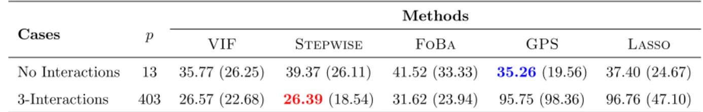
remaining piece. The results are summarized in Table 4. Not surprisingly, stepwise regression gave the best performance overall, since it tries to build thesparsest possible model with strong collective predictability, and thus it will not suffer much from the multicollinearity. The strong multicollinearity, however, caused trouble for GPS, the leader in the case without interactions. One possible explanation is that due to the strong collinearity, GPS had a hard time making a unified decision on the working penalty for the different folds. This variability in the penalties caused a much larger variance in the model performances. As a result, the test errors tend to be large and have a high variance, as shown in Table 4. The same problem happened to Lasso, which could only do well with small p and weak collinearity. VIF regression did well in both cases because it tried to approximate the searching path of stepwise regression; the slightly higher errors were the price it paid for the substantially improved speed.
[Table 4 about here.]
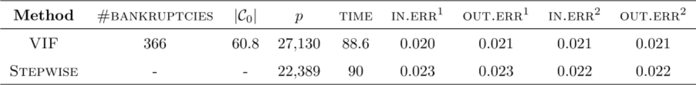
7.2 Bankruptcy Data
We also applied VIF Regression to the bankruptcy data that was originally used in Foster and
Stine (2004). This sample data contains 20,000 accounts and 147 features, 24 of which are
categorical. It has substantial missing data. It is well understood that missing data serves to characterize the individual account behaviors (Jones 1996); i.e., knowing which data are missing improves model predictivity. Hence, instead of filling in with expected values based on the observed data, we use an indicator for each of them as in Foster and Stine (2004). We also decompose each of the 24 categorical variables that have categories (l) greater than two intol−1 dummy variables. Hence, in total, we have 439 features for our linear model. To dynamically select interaction terms, we first apply VIF regression on the 439 linear features to get a baseline subset C0. We then apply VIF regression with sub-sampling size m = 400 on the interaction terms of the selected variables inC0 and all the features. The total number of candidate variables we considered was thus p= (|C0|+ 1)×439, as summarized in Table 5.
[Table 5 about here.]
To gauge the classification performance, we perform a five-fold cross validation and employ the 0-1 loss function to compute the in-sample and out-of-sample classification error for each fold. We compared two different cutoff rules ξ1 = 1−#bankruptcies/nCV, where#bankruptcies is the number of bankrupt accounts in sample, and ξ2 = 8/9.
We also compared with stepwise regression by generating 22,389 predictors and using stepwise regression to pick variables. Given a time limit of 90 minutes, stepwise regression could only select (on average) 4 variables compared to 400 features selected by VIF. We were not able to run the other three algorithms on this data.
7.3 Call Center Data
The call center data we are exploring in the section are collected by an Israeli bank. On each day, the number of calls to the customer center was counted every 30 seconds. This call value is the dependent variable to be predicted. The data was collected from November 1st, 2006 to April 30th, 2008, 471 days in total (a few days are missing). Hence, we have in total n = 1,356,480 observations. Similar data sets have been investigated inBrown et al.(2005) andWeinberg et al.
(2007).
In order to have approximately normal errors, we performed a variance stabilization trans-formation (Brown et al. 2005) to the number of counts N:
y=pN + 1/4.
The variables we are investigating for possible inclusion in the model include day of week
{xd}6d=1, time of dayφ
f
t and ψ f
t , and lagsyt−k. For time of day, we consider Fourier transforms
φft = sin 2πf ·t ω and ψft = cos 2πf ·t ω ,
interactions between day of week and time of day,{φft·xd}and{ψtf·xd}as explanatory variables.
This results in a set of 2,054 base predictors and 12,288 interactions.
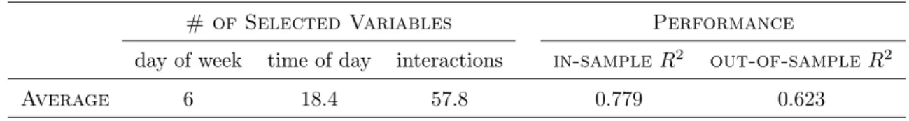
We again did a five fold cross validation to test our performance. Our VIF regression selected on average 82 of the features and gave an in-sample R2 of 0.779 and an out-of-sample R2 of 0.623. The features selected were primarily interactions between the day of week and the time of day as summarized in Table 6.
[Table 6 about here.]
Note that the in-sample performance is better than the out-of-sample performance because of the autoregressive nature of this data. The feature selection criteria we used only guarantees that there will be no overfitting for the case of independent observations. For non-independent observations, the effective sample size is smaller than actual number of observations, and hence adjusted criteria should be taken into account. We also considered adding auto-regressive effects, i.e., lag variables {yt−k}, in the model; we gained both in-sample and out-of-sample R2 as high
as 0.92. However, in the typical use of models of call center data, estimating number of calls in order to determine staffing levels, {yt−k} is not available at the time that the staffing decisions
need to be made, and so cannot be used for prediction. The speed and flexibility of our algorithm enable us to efficiently extract informative relationships for such a large scale data.
8 DISCUSSION
Fast and accurate variable selection is critical for large-scale data mining. Efficiently finding good subsets of predictors from numerous candidates can greatly alleviate the formidable computation task, improve predictive accuracy, and reduce the labor and cost of future data collection and experiment design. Among a variety of variable selection algorithms, stepwise regression is empirically shown to be accurate but computationally inefficient; l1 and lε algorithms are less
accurate in highly sparse systems. In this paper, we proposed a hybrid algorithm, VIF regression, that incorporates a fast and simple evaluation procedure. VIF regression can be adapted to
various stepwise-like algorithms, including a streamwise regression algorithm using anα-investing rule. Due to the one-pass nature of the streamwise algorithm, the total computational complexity of this algorithm can be reduced toO(pn), as long as the subsample sizem=O(n/q2), which can be easily achieved in large-scale datasets. Furthermore, by employing an α-investing rule, this algorithm can control mFDR and avoid over-fitting. Our experimental results demonstrate that our VIF algorithm is substantially as accurate as, and is faster than other algorithms for large scale data. Based on these results, we believe that the VIF algorithm can be fruitfully applied to many large-scale problems. VIF regression code in R is available at the CRAN repository (http://www.r-project.org/).
References
Benjamini, Y. and Hochberg, Y. (1995), “Controlling the False Discovery Rate: a Practical and Powerful Approach to Multiple Testing,” Journal of the Royal Statistical Society, Ser. B, 57, 289–300.
Breiman, L. and Freedman, D. (1983), “ How many variables should be entered in a regression equation?” Journal of the American Statistical Association, 78, 131–136.
Brown, L., Gans, N., Mandelbaum, A., Sakov, A., Shen, H., Zeltyn, S., and Zhao, L. (2005), “Statistical Analysis of a Telephone Call Center: A Queueing-Science Perspective,” Journal of the American Statistical Association, 100, 36–50.
Cai, T. and Wang, L. (2010), “Orthogonal Matching Pursuit for Sparse Signal Recovery,” Tech-nical Report, University of Pennsylvania.
Candes, E. J. and Tao, T. (2007), “The Dantzig Selector: Statistical Estimation Whenpis much larger thann,”The Annals of Statistics, 35.
Efron, B., Hastie, T., Johnstone, I., and Tibshirani, R. (2004), “Least Angle Regression (with discussion),”The Annals of Statistics, 32.
Efron, B., Tibshirani, R., Storey, J. D., and Tusher, V. (2001), “Empirical Bayes Analysis of a Microarray Experiment,” Journal of the American Statistical Association, 96, 1151–1160. Foster, D. P. and Stine, R. A. (2004), “Variable selection in data mining: building a predictive
model for bankruptcy,” Journal of the American Statistical Association, 99, 303–313.
— (2008), “Alpha-investing: a procedure for sequential control of expected false discoveries,”
Journal of the Royal Statistical Society, Ser. B, 70.
Friedman, J. H. (2008), “Fast Sparse Regression and Classification,” Technical Report, Standford Univerisity.
Friedman, J. H., Hastie, T., and Tibshirani, R. (2010), “Regularization Paths for Generalized Linear Models via Coordinate Descent,” Journal of Statistical Software, 33, 1–22.
Greenshtein, E. and Ritov, Y. (2004), “Persistency in High Dimensional Linear Predictor-Selection and the Virtue of Over-Parametrization,”Bernoulli, 10, 971–988.
Guyon, I. and Elisseeff, A. (2003), “An Introduction to Variable and Feature Selection,”Journal of Machine Learning Research, 3, 1157–1182.
Hastie, T., Tibshirani, R., and Friedman, J. (2009), The Elements of Statistical Learning, Springer-Verlag, 2nd ed.
Jones, M. P. (1996), “Indicator and Stratification Methods for Missing Explanatory Variables in Multiple Linear Regression,”Journal of the American Statistical Association, 91, 222–230. Konishi, S. (1978), “An Approximation to the Distribution of the Sample Correlation
Coeffi-cient,” Biometrika, 65, 654–656.
Lin, D., Foster, D. P., Pitler, E., and Ungar, L. H. (2008), “In Defense of l0 Regularization,”
Miller, A. (2002), Subset Selection in Regression, Chapman and Hall, 2nd ed.
Natarajan, B. K. (1995), “Sparse approximate solutions to linear systems,” SIAM Journal on Computing, 24, 227–234.
Storey, J. D. (2002), “A Direct Approach to False Discovery Rates,” Journal of the Royal Sta-tistical Society, Ser. B, 64, 479–498.
Tibshirani, R. (1996), “Regression Shrinkage and Selection via the Lasso,” Journal of the Royal Statistical Society, Ser. B, 58, 267–288.
Tropp, J. A. (2004), “Greed is Good: Algorithmic Results for Sparse Approximation,” IEEE Transactions on Information Theory, 50, 2231–2242.
Wang, H. (2009), “Forward Regression for Ultra-high Dimensional Variable Screening,” Journal of the American Statistical Association, 104, 1512–1524.
Weinberg, J., Brown, L. D., and Stroud, J. R. (2007), “Bayesian Forecasting of an Inhomogeneous Poisson Process With Applications to Call Center Data,” Journal of the American Statistical Association, 102, 1185–1198.
Zhang, T. (2009), “Adaptive Forward-Backward Greedy Algorithm for Sparse Learning with Linear Models,” in Advances in Neural Information Processing Systems 21, Cambridge, MA: MIT Press, pp. 1921–1928.
Zhou, J., Foster, D. P., Stine, R. A., and Ungar, L. H. (2006), “Streamwise Feature Selection,”
Table 1: True |ρ|’s in the Boston Data. We added these variables into our multiple linear regression
model sequentially. Displayed are the|ρ|values when the corresponding variable is added in the model.
These |ρ|’s are computed using (6).
CRIM ZN INDUS CHAS NOX RM AGE
1.00 0.98 0.79 0.99 0.62 0.90 0.64
DIS RAD TAX PTRATIO B LSTAT
Table 2: Summary of the average numbers of true discoveries, false discoveries, and estimated mFDR using the five algorithms in the experiment with independent Gaussian features. The training set
contained 1,000 observations and p features, six of which were used to create the response variables.
This simulation was repeated 50 times.
Methods Cases
VIF Stepwise FoBa GPS Lasso true 6.0 6.0 6.0 6.0 5.86 p= 100 false 0.82 0.02 0.04 0.18 38.82 mFDR 0.049 0.001 0.002 0.011 0.710 true 6.0 6.0 6.0 6.0 5.38 p= 200 false 0.56 0.04 0.02 0.08 70.02 mFDR 0.034 0.002 0.001 0.005 0.820 true 6.0 6.0 6.0 6.0 5.66 p= 300 false 0.60 0.06 0.02 0.04 75.44 mFDR 0.036 0.004 0.000 0.002 0.828 true 6.0 6.0 6.0 6.0 5.50 p= 400 false 0.56 0.10 0.00 0.02 93.78 mFDR 0.034 0.006 0.000 0.001 0.858 true 6.0 6.0 6.0 6.0 5.48 p= 500 false 0.58 0.04 0.00 0.04 117.78 mFDR 0.035 0.002 0.000 0.002 0.884
Table 3: Summary of the average numbers of true discoveries, false discoveries, and estimated mFDR using the five algorithms in the experiment with jointly Gaussian features. The training set contained
1,000 observations and 200 features, six of which were used to create the response variables. The θ in
(17) were taken to be 0.1, 0.3, 0.5, 0.7 and 0.9. This simulation was repeated 50 times.
Methods Cases
VIF Stepwise FoBa GPS Lasso true 6.00 6.00 6.00 6.00 5.64 θ= 0.1 false 0.56 0.02 0.02 0.26 72.94 mFDR 0.034 0.001 0.001 0.016 0.823 true 6.00 6.00 6.00 6.00 5.54 θ= 0.3 false 2.04 0.02 0.02 0.12 68.40 mFDR 0.113 0.001 0.001 0.007 0.815 true 6.00 6.00 6.00 5.90 5.86 θ= 0.5 false 6.30 0.04 0.10 0.20 74.12 mFDR 0.282 0.002 0.006 0.012 0.824 true 6.00 6.00 6.00 6.00 5.84 θ= 0.7 false 13.20 0.04 0.16 0.60 64.58 mFDR 0.452 0.002 0.010 0.036 0.803 true 5.46 5.66 5.46 5.84 5.90 θ= 0.9 false 32.30 0.33 0.64 2.44 76.22 mFDR 0.676 0.019 0.038 0.133 0.827
Table 4: Boston Data: average out-of-sample mean squared error in a five-fold cross validation study. Values in parentheses are the standard error of the these average mean squared errors.
Methods
Cases p
VIF Stepwise FoBa GPS Lasso
No Interactions 13 35.77 (26.25) 39.37 (26.11) 41.52 (33.33) 35.26(19.56) 37.40 (24.67) 3-Interactions 403 26.57 (22.68) 26.39(18.54) 31.62 (23.94) 95.75 (98.36) 96.76 (47.10)
Table 5: Bankruptcy Data. The performance of VIF and stepwise regression on a five-fold cross valida-tion.
Method #bankruptcies |C0| p time in.err1 out.err1 in.err2 out.err2
VIF 366 60.8 27,130 88.6 0.020 0.021 0.021 0.021
Stepwise - - 22,389 90 0.023 0.023 0.022 0.022
* time: CPU running time in minutes
* in.err1/out.err1: In-sample classification errors/Out-of-sample classification errors usingξ1
* in.err2/out.err2: In-sample classification errors/Out-of-sample classification errors usingξ2
Table 6: Call Center Data. The performance of VIF and selected variables on a five-fold cross validation.
# of Selected Variables Performance
day of week time of day interactions in-sampleR2 out-of-sampleR2
Average 6 18.4 57.8 0.779 0.623
List of Figures
1 Number of candidate variables examined (“capacity”) of five algorithms: VIF
Regression, Stepwise Regression, Lasso, FoBa, and GPS, within fixed time (in seconds). The algorithms were asked to search for a model givenn= 1,000 obser-vations and p candidate predictors. VIF regression can run many more variables than any other algorithm: by the 300th second, VIF regression has run 100,000 variables, while stepwise regression, Lasso and FoBa have run 900, 700 and 600 respectively. The implementation of GPS stopped when p is larger than 6,000; nevertheless, it is clear that VIF regression can run on much larger data than GPS could. Details of the algorithms and models are given in Section 6. . . 42
2 Out-of-sample mean squared errors of the models chosen by the five algorithms. The algorithms were asked to search for a model givenn= 1,000 observations and
p= 500 independently simulated candidate predictors; mean squared errors of the five chosen models on a test set were computed. We repeated this test 50 times and in the figure are the boxplots of these results. VIF regression is as accurate
as stepwise regression and FoBa, and much more accurate than GPS and Lasso. . 43
3 A schematic illustration of Proposition 1. Suppose y = βx+βnewxnew+ε. Let
Px denote the projector on x, then r = y−Pxy and Px⊥xnew = xnew −Pxxnew.
In stepwise regression, the model fit is the projection of r on Px⊥xnew while in
stagewise regression, the model fit is the projection of r on xnew. Note that the
red dotted line is perpendicular toxnew and the red dashed line is perpendicular
toPx⊥xnew, ˆγnew/βˆnew=hxnew,P⊥xxnewi2/kxnewk2kP⊥xxnewk2 =hxnew,P⊥xxnewi=ρ2. 44
4 The biased t-ratio. We simulated y = x+xnew+N(0,1) with sample size n =
30, Corr(x,xnew) =
p
1−ρ2. For each ρ varying from 0 to 1, we computed
both t-statistics of the estimated coefficient of xnew, tstage and tstep, from the two
procedures. Shown in the plot is the ratio tstage/tstep on ρ. It matches ρ well, as
suggested by (9). . . 45
5 Out of Sample Errors of three algorithm. A na¨ıve algorithm without correction may not be as accurate. . . 46
6 Simulation of |ˆt|for the Boston Data. We added these variables into our multiple linear regression model sequentially. For each variable, the approximate t-ratio |ˆt| = |ˆγnew|/σˆ|ρˆ| was computed based on a sub-sample of size m = 200. These boxplots result from a simulation of 100 subsample sets. Annotated below the variables are the true |ρ|’s. . . 47
7 Running Time (in seconds) of the five algorithms: VIF Regression, Stepwise Re-gression, Lasso, FoBa, and GPS. The algorithms were asked to search for a model given n= 1,000 observations andp candidate predictors; pvaries from 10 to 1,000. 48
8 Running Time (in seconds) of VIF Regression and GPS algorithm. The algorithms
were asked to search for a model given n = 1,000 observations and p candidate predictors; p varies from 10 to 10,000. . . 49
9 Out-of-sample mean squared errors of the models chosen by the five algorithms
in the simulation study with independent distributed features. The number of features p varied from 100 to 500 (from left to right in the figure). . . 50