Approximation of ruin probability using phase-type distributions

(1)

UNIVERSITY OFTARTU

FACULTY OF SCIENCE ANDTECHNOLOGY INSTITUTE OFMATHEMATICS AND STATISTICS

KIRILLSMIRNOV

Approximation of Ruin Probability

using Phase-Type Distributions

ACTUARIAL ANDFINANCIAL ENGINEERING MASTER’STHESIS (30 ECTS)

SUPERVISOR: PROF. KALEVPÄRNA

(2)

Laostumistõenäosuse lähendamine faas-tüüpi jaotuste abil Magistritöö

Kirill Smirnov

Lühikokkuvõte.Käesoleva magistritöö eesmärk on leida laostumistõenäosuse lähend, mis on täpsem, kui hästituntud De Vylderi meetod, aga samal ajal on matemaatiliselt lihtne. Töös esitatud uus lähendusmeetod kaustab ära De Vylderi meetodi idee, kuid eksponetjaotuse asemel kasutab faas-tüüpi jotusi. Töö teoreetilises osas antakse ülevaade riskiprotsessidest, faas-tüüpi jaotustest ja De Vylderi meetodist ning tuletatakse valemid faasi-tüüpi lähendjaotuse parameetrite arvutamiseks. Töö praktilises osas võrreldakse kuue uudse lähendusmeetodi täpsust De Vylderi meetodi täpsusega. Võrdlemine toimub numbriliselt nelja erinevate riskiprotsessi põhjal ning tulemused näitavad uute meetodite suuremat täpsust võrreldes De Vylderi meetodiga.

CERCS teaduseriala:P160 Statistika, operatsioonanalüüs, programmeerimine, finants-ja kindlustusmatemaatika.

Märksõnad:Riskiteooria, laostumistõenäosus, faas-tüübi jaotus, risksprotsees, ekspo-nentjaotus, De Vylderi meetod.

Approximation of Ruin Probability using Phase-Type Distributions Master’s thesis

Kirill Smirnov

Abstract. The purpose of this master’s thesis is to find an approximation of ruin proba-bilities that is more accurate than well-known De Vylder’s method, but at the same time is mathematically simple enough. This new approximation method is based on the idea of De Vylder’s approximation, but instead of exponential distribution of claims some more complicated phase-type distributions are used. In theoretical part of the thesis an overview of main concepts of risk theory, the notion of phase-type distribution and De Vylder’s approximation is given. In practical part accuracy of six approximations of ruin probability based on phase-type distributions are compared with De Vylder’s method. The comparison is based on numerical examples of four different risk processes. Accord-ing to the results, new methods are more accurate than De Vylder’s approximation. CERCS research specialisation: P160 Statistics, operation research, programming, actuarial mathematics.

Keyword: Risk theory, ruin probability, phase-type distribution, risk process, exponen-tial distribution, De Vylder’s approximation.

(3)

Introduction

The main question of classical risk theory is the calculation of the ruin probability of an insurance company. One of the factors affecting the probability of ruin is the claim distribution. There is a whole list of distributions fitting claim sizes depending on the type of insurance. Unfortunately, it is not possible to evaluate the exact formula of the ruin probability for most of claim distributions. One possibility to estimate the ruin probability, if the exact formula is not available, is using of approximations.

One of the most famous and successful approximations is De Vylder’s approxima-tion. The idea of this method is very simple. Assume that it is not possible to calculate the exact ruin probability for some distribution of claims. Than it is needed to replace initial distribution with well-fitting exponential one and calculate the ruin probability using the exact formula for exponentially distributed claims.

Exponential distribution is the simplest case of phase-type distributions and exact for-mula of the ruin probability for exponentially distributed claims can be expanded for all phase-type distributions. Hence, an idea has sparked to modify De Vylder’s approxi-mation by using phase-type distributions instead of exponential distribution. Intuitively, more complicated phase-type distribution will give more accurate estimation of the ruin probability. From here follows the main goal of the thesis: to find more accurate but at the same time mathematically simple enough approximation of the ruin probability based on phase-type distribution using the idea of De Vylder’s method.

The main part of this thesis is divided into four chapters. In Chapter 1 we study the main basic concepts of the classical risk theory that are needed in the future research. Chapter 2 is devoted to De Vylder’s approximation. Here is given a brief explanation of the method’s idea and shown its application based on three numerical examples. In Chapter 3 we meet up with the notion of phase-type distributions, consider main special cases of this class of distributions and modify De Vylder’s method using six different phase-type distributions. In the last chapter we apply received modifications of De Vylder’s methods on the examples from the Chapter 2.

Most of the calculations in the thesis are done using software: RStudio 3.3.1; Max-ima 5.42.2.

(5)

1 Main concepts and results of classical risk theory

In this chapter we will give a brief explanation of main concepts of classical risk theory, such as stochastic processes, ruin probability and classical risk model. This chapter is mainly based on [1] and [2].

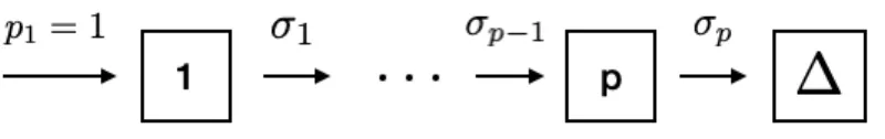
1.1 The classical risk model

Let’s consider the main cash-flows of an insurance company. The finance operations of insurer can be presented as a series of inflows and outflows (Figure 1). The main source of income for this business segment is selling of premiums. Also, insurer receive money through reinsurance recoveries, investments, etc. The main outflows are claims payout, reinsurance premiums, dividends paid to shareholders and bonuses paid to policyholders. The most important component of an insurance company’s expenses is usually payout of claims.[5]

Figure 1. Main cash-flows of an insurance company

The number of claims arriving during the time interval and their sizes are usually un-known and can take different values i.e. they are stochastic. That is why the amount of outflows is changeable and at different moments of time can exceed the inflows amount or not.

(6)

From the changeability of the outflows follows the main classical question of the risk theory - to study the ruin probability of a company, i.e. the probability that company’s balance will become negative at some point of time.

Definition 1.1. Stochastic processis defined as a family of random variables{X(t) :

t∈T}, wheretis time parameter andT is the set of possible values oft. The setT can be discrete (T ={1,2, . . .}) or continuous (T = [0,∞)).

Counting process is a special case of stochastic processes. Let us consider an eventA

that happens at random time pointsS1,S2,. . . The number of occurrences ofAwithin

the time interval[0, t]is called a counting process:

N(t) = #{i:Si ∈[0, t]}.

So the number of claimsN(t)arriving within the time interval[0, t]is a counting process. Now we can formulate the definition of the standard risk model.

Definition 1.2. Risk processis a stochastic process defined as

X(t) = ct− N(t) X k=1 Zk, (1) where

• c- positive real constant meaning gross premium rate i.e. company receives c money units per time unit;

• N(t) - counting process with N(0) = 0, interpreted as the number of claims arrived within the time interval(0, t];

• {Zk}∞k=1 - sequence of independent and identically distributed random variables

with mean valueµ, and varianceσ2. Zkmeans the size ofk−th claim.

This is the standard risk model of an insurance company, which is interpreted as follows. An insurer receivescmoney units per time unit and loses random amounts of moneyZ1,

Z2,. . .,ZN(t)at time pointsS1,S2,. . .,SN(t) ∈(0, t]. Hence, risk processX(t)means

the profit of a company within the time period(0, t].

(7)

waiting timesTiof the events as time difference between current and previous occurrence of the event:

Ti =Si−Si−1.

Definition 1.3. A counting processN(t)is calledPoisson processif its waiting times

T1,T2,. . . are independent random variables from the same exponential distribution

with rate parameterα. The parameterαis called the intensity of the Poisson process. The classical risk theory is based on the Poisson process.

Definition 1.4. Risk processX(t)is calledclassical risk processif counting process

N(t)is Poisson process.

Further in this thesis we consider only classical risk processes.

Assume that N has intensity α. It means, E(N(t)) = αt. Hence, expected profit of the company within time period(0, t]is

E(X(t)) =E(ct)−E(N(t))·E(Zk)) =ct−αµt= (c−αµ)t.

The ratio c−_αµαµ is called relative safety loading, denoted byρ. If relative safety loading is positive (ρ > 0), then the risk processX(t)has a drift to+∞and it is said that the company is profitable.

Usually, the company starts its activities having some starting capital u. Now we can define the main concept of classical risk theory - ruin probability - for an insurance company with the risk processX(t)described by equation(1)and starting capitalu. Definition 1.5. The ruin probabilityof an insurance company with initial capitalu

and risk processX(t)is a probability, that at some time pointt >0company’s balance

u+X(t)will be negative.

Ψ(u) = P{u+X(t)<0for somet >0}.

From here follows the definition of non-ruin probability Φ(u) which is defined as 1−Ψ(u).

(8)

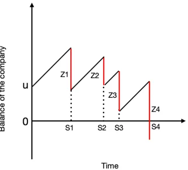
Figure 2. Illustration of a risk process’s trajectory

The concept of the risk process is clearly illustrated in Figure 2. Starting with initial capitaluat timet = 0the company receivescmoney units per time unit. In this way company’s balance is equal tou+c·S1 at the time point S1, before the first claim’s

arrival. Paying out the claim company’s balance decreases byZ1. So the profit of the

company within the time interval(0, S1]is equal toc·S1−Z1. After that the process

repeats. At the time pointS4 the fourth claimZ4arrives. The size of claim is greater than

the current balance of the company. Hence, paying out of this claim leads to reserve’s drop below zero. It means that at the timeS4 accrues ruin of observed company.

1.2 Exact formula of the ruin probability for exponentially distributed

claims

As it was mentioned in the previous section, the main classical question of the theory of risks is the calculation of the ruin probability. The ruin probability depends on the starting capital, the intensity of Poisson process and the distribution of claims. In this

(9)

section we consider the risk process with exponentially distributed claims and derive the exact formula of the ruin probability for this case.

Theorem 1.1. If claim sizes Zk of the classical risk process X(t) are exponentially distributed, i.e.Zk ∼Exp(σ), then the ruin probabilityΨ(u)can be calculated by the following formula: Ψ(u) = 1 1 +ρ ·exp − ρu µ(1 +ρ) ,

whereµ= 1_σ is mean value of exponential distribution andρ= c−_αµαµ is relative safety loading.

In order to prove this theorem, we need to derive some other important results of the classical theory of risks.

Let’s consider the classical risk processXfor a company with an initial capital equal tou. Suppose that the first claimZ1 arrives at the time momentS1, thenX(S1) = c·S1−Z1.

In this way, at timeS1 starts, so say, a "new" risk processXwith an initial capital equal

tou+c·S1−Z1.

Since we assume, that ruin can not happen within time interval(0, S1):

Φ(u) =E(Φ(u+c·S1−Z1)) = Z ∞ 0 Z ∞ 0 Φ(u+cs−z)dF(z)dFS1(s),

whereFS1(s)andF(z)are distribution functions ofS1 andZ1 respectively.

As we consider classical risk process, S1 is exponentially distributed with intensity

α. Hence,dFS1(s) = α·e −αs_ds_. Φ(u) = Z ∞ 0 α·e−αs Z ∞ 0 Φ(u+cs−z)dF(z)ds.

If the claim size is greater or equal tou+cs, occurs ruin of the company at timeS1.

Assuming that, we get Φ(u) = Z ∞ 0 α·e−αs Z u+cs 0 Φ(u+cs−z)dF(z)ds.

Let’s apply the change variablex:=u+cs. It follows, thatds = ds_c. Φ(u) = α c ·e αu c Z ∞ u α·e−α·xc Z x 0 Φ(x−z)dF(z)dx.

(10)

Differentiating ofΦbyuwe get Φ0(u) = α 2 c2 ·e αu c Z ∞ u α·e−α·xc Z x 0 Φ(x−z)dF(z)dx−α c·e α·u c ·e− α·u c Z u 0 Φ(u−z)dF(z).

The first term of the right side is equal to α_cΦ(u). Then we get Φ0(u) = α cΦ(u)− α c Z u 0 Φ(u−z)dF(z). (2) Integration of the received equation over(0,uˆ)leads to

Φ(û)−Φ(0) = α c Z uˆ 0 Φ(u)du+ α c Z û 0 Z u 0 Φ(u−z)·(1−F(z))du= α c Z uˆ 0 Φ(u)du+ α c Z uˆ 0 Φ(0)·(1−F(u))−Φ(u) + Z u 0 Φ0(u−z)d(1−F(z))dz du= α cΦ(0) Z û 0 (1−F(u))du+α c Z uˆ 0 (1−F(z))dz Z uˆ z Φ0(u−z)du = α cΦ(0) Z uˆ 0 (1−F(u))du+α c Z uˆ 0 (1−F(z))dz(Φ(û−z)−Φ(0))dz.

From here we get the final integral equation for non-ruin probability: Φ(u) = Φ(0) + α

c

Z u

0

Φ(u−z)·(1−F(z))dz. (3) Assume now that initial capital tends to infinity (u→ ∞) and the company is profitable (ρ >0). It is possible to show using Monotone Convergence Theorem that in this case equation3leads to

Φ(∞) = Φ(0) + αµ

c Φ(∞). (4)

Ifρis positive, thenlimt→∞X(t) = +∞a.s. Hence there is timeT, such that for all

time momentst > T profit of the company is positive (X(t)>0). It means that ruining of the company can not occur after the timeT. Consider the time period[0, T]. Within this time interval arrives finite number of claims (N(T)is Poisson process) and the size of each claim is finite too. These facts lead to conclusion that total sum of expenses

(11)

(PN_k₌₁(T)Zk) is finite. Therefore, having infinite initial capital, company can not ruin in period[0, T]. We have shown that the ruin probability of the company in this case is equal to zero in time interval[0, T]and for allt > T. From here follows thatΦ(∞) = 1. Substituting this result into equation (4) we get

1 = Φ(0) + αµ

c .

AsΨ(u) = 1−Φ(u)and using the definition of relative safety loadingρwe get Ψ(0) = αµ

c =

1 1 +ρ.

Now we have got all needed results to prove the theorem1.1. Proof of the Theorem 1.1:

Let’s find the ruin probability of a company with an initial capitalu, assuming that claims are exponentially distributed with the mean valueµ.

Distribution function of exponential distribution F(z) is 1 − e−zµ_{. It follows that} dF(z) = _µ1e−µzdz. Substituting this result into the equation2we get

Φ0(u) = α cΦ(u)− α cµ Z u 0 Φ(u−z)·e−zµ_dz.

Let’s apply change variablev :=u−z. It followsdz =−dv. Φ0(u) = α cΦ(u)− α cµ Z u 0 Φ(z)·e−u−µzdz.

Differentiation and simplification of this equation leads to Φ00(u) = α cΦ 0 (u) + 1 µ α µΦ(u)−Φ 0 (u) − α cµΦ(u) = = α c − 1 µ ·Φ0(u) =− ρ µ(1 +ρ) ·Φ 0 (u).

(12)

Φ00(u) Φ0₍_u₎ =− ρ µ(1+ρ). Hence, ln Φ0(u) =− ρ µ(1 +ρ) ·u+C1, Φ0(u) =eC1 _·_exp − ρ µ(1 +ρ) ·u =C2·exp − ρ µ(1 +ρ)·u , Φ(u) =C3·exp − ρ µ(1 +ρ)·u +C4.

We have proved above thatΦ(∞) = 1andΦ(0) = 1− 1

1+ρ. Using these results we can findC3andC4 values:

   1− 1 1+ρ =C3·exp − ρ µ(1+ρ) ·0 +C4 1 =C3·exp −_µ₍₁₊ρ_ρ₎· ∞+C4 .

From the second equation of the system follows: 1 = C3 ·0 +C4,

C4 = 1.

SubstitutingC4into first equation of the system we get:

1− 1 1 +ρ =C3·1 + 1, C3 =− 1 1 +ρ. Therefore, Ψ(u) = 1−Φ(u) = 1 1 +ρexp − ρu µ(1 +ρ) .

In many scientific articles it is customary to assign gross premium rate c equal to one for simplicity. It means that c is taken as money unit and all other quantities (including claims sizes) are measured in this units.[3] Assume that we have a risk process

X(t) = c·t−PN_k₌₁(t)Zk withc 6= 1. We can define a new risk process Xˆ(t) = X_c(t) which has gross premium rateˆc= 1:

ˆ X(t) = ct c − N(t) X k=1 Zk c = 1·t− N(t) X k=1 Zk c .

(13)

According to the definition of ruin probability is easy to show thatψ(u) = ˆψ(u). Thus, we can present the risk process with any gross premium rate, as a new risk process with

c= 1, which has the same ruining probabilities as initial process. Using this property we can simplify the result of Theorem1.1.

Ψ(u) = 1 1 + 1−_αµαµ ·exp − 1−αµ αµ ·u µ(1 +ρ) ! =αµ·exp − 1 µ−α ·u . (5)

Further in this thesis we assume that gross premium rate is equal to one,c= 1.

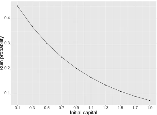
Example 1.1. Let’s consider an insurance company with initial capital u = 0.1 and gross premium ratec= 1. Assume that claims are exponentially distributed with mean valueµ= 0.5and intensity of Poisson processα= 1.

In this case we can calculate the probability of ruining using equation (5). Ψ(0.1) = 1·0.5·exp − 1 0.5 −1 ·0.1 = 0.5·exp (−0.1)≈0.45242 Thus, starting with 0.1 money units on its balance the company will ruin with probability 0.45. Obviously, increasing initial capital of the company the ruin becomes less likely. This process is shown in Figure3. For example, if the company increases its starting capital up to 1.9 money units, the ruining probability will be 0.0748.

(14)

Figure 3. Ruin probability for different values of initial capital

The exact formula of the ruin probability in case of exponentially distributed claims is very simple and convenient in application. But the risk process with exponentially distributed claims is just one rare example of risk processes where an exact formula exists. For example, Cramer-Lundberg approximation (6) does not work in case of heavy-tailed distributions. lim u→∞Ψ(u)·e −Ru ₌ ρu h0₍_R₎₋ c α , (6)

whereRis positive constant (Lundberg exponent) andh(r) = R∞

0 e

(15)

2 De Vylder’s approximation for the ruin probabilities

As it was shown in the previous chapter, it is possible to calculate exact ruin probabili-ties of risk processes with exponentially distributed claims, occurring according to the Poisson process. But exponential distribution is not the only possible distribution used to describe sizes of claims. There is a whole list of distributions - that fit the data much better in different situations. For example, in non-life insurance exponential distribution is considered to be not enough realistic for using in real life models and preferences are given to other distributions, such as Gamma, Weibull and Lognormal.[5]

There are some other claim’s distributions besides exponential one, where exact formula of the ruin probability can be derived, for example, class of phase-type distributions. But in most case of claim distributions the ruin probability can be calculated only via simulation process or using some approximations.

Several approximations to the ruin probability have been proposed. The most famous of them are Cramer-Lundberg’s, Beekman-Bowers’s and De Vylder’s approximations. Futher we will focus on the De Vylder’s method of finding of ruin probabilities. This chapter is mostly based on [1], [2] and [6].

2.1 Concept of De Vylder’s method

De Vylder’s approximation (1978), is the most successful and mathematically simple approximation of the ruin probability. Consider the risk process X(t) having such distribution of claims, that it is not possible to calculate exact ruin probability of it. Assume that the intensity of Poisson process isα, and the gross premium rate isc. De Vylder’s method is based on the idea to replaceX(t)with a new risk processXˆ(t)having exponentially distributed claims, such that the first three moments ofX(t)match with the first three moments ofXˆ(t). It means

E[Xk(t)] =E[ ˆXk(t)] fork= 1,2,3.

The number three comes from the fact that the risk process with exponentially distributed claims has three parameters: the premium gross rateˆc, the rate of exponential distribution ˆ

(16)

When parameters of Xˆ(t) are estimated, it is possible to calculate the ruin probabil-ity of this process, which is approximately equal to the ruin probabilprobabil-ity ofX(t)

Ψ_Xˆ₍_t₎(u)≈ΨX(t)(u).

To derive the first three moments ofX(t)the characteristic function is used.

Definition 2.1. [8]For a scalar random variableXthe characteristic functionis defined as the expected value ofeivX_{, where}_i_{is the imaginary unit, and}_v _∈

Ris the

argument of the characteristic function:

ϕ(v) = E

eivX

.

For simplicity of the calculations we take the logarithm of characteristic function (or characteristic exponent) ofX(t):

log EeivX(t)= log E eiv ct−PN(t) k=1 Zk =t icv+α Ee−ivZk₋₁_.

According to the Taylor seriesex=P∞ n=0 xn n!. Hence, e−ivZk ₌ 3 X n=0 (−ivZk)n n! +o(v) 3 = 1 + (−ivZk) 1 + (−ivZk)2 2 + (−ivZk)3 6 +o(v) 3 = 1−ivZk− v2_Z2 k 2 + iv3_Z3 k 6 +o(v) 3_. Hence, Ee−ivZk_{= 1}₋_ivζ 1− v2_ζ 2 2 + iv3_ζ 3 6 +o(v) 3_,

whereζ1, ζ2, ζ3are the first three moments of claim distributionZk respectively. Then log EeivX(t)= =t icv+α 1−ivζ1 − v2ζ2 2 + iv3ζ3 6 +o(v) 3₋ 1 = =t iv(c−αζ1)− v2_ζ 2α 2 + v3_iαζ 3 6 +o(v) 3 .

(17)

Taking exponent of both sizes of the last equation we get characteristic function of the risk processX(t). ϕX(t)(v) =E eivX(t) = = exp t iv(c−αζ1)− v2_ζ 2α 2 + v3_iαζ 3 6 +o(v) 3 .

Property 2.1. [8] If a random variable X has moments up to k-th order, then the characteristic functionϕX isktimes continuously differentiable on the entire real line. In this case

E Xk=i−k·ϕ(k)(0).

Using Property2.1we can derive expressions of the first moments ofX(t) :

E[X(t)] =i−1ϕ0(0) = i−1t i(c−αζ1)−vζ2α+ v2iαζ3 2 ϕX(t)(v) v=0 = =i−1·i·t(c−αζ1)e0 =t(c−αζ1).

Same result was obtained in the section 1.1. The second and the third moments ofX(t) can be derived in the same way. As a result, we get

E[X(t)] =t(c−αζ1),

EX2(t)=αζ2t+ (c−αζ1)2t2,

E

X3(t)

=−αζ3t+ 3(c−αζ1)(αζ2)t2+ (c−αζ1)3t3.

Since the claims ofXˆ(t)are exponentially distributed, then-th moment ofZkcan be found as follow: E[Z_kn] = n! ˆ σn. Hence, ˆ ζ1 =E[Zk] = 1 ˆ σ, ˆ ζ2 =E Z_k2= 2 ˆ σ2, ˆ ζ3 =E Z_k3= 6 ˆ σ3.

(18)

Thus, to match the first three moments ofX(t)andXˆ(t)parametersσˆ,cˆ,αˆmust satisfy the next system of equations.

       c−αζ1 = ˆc−αˆ1_ˆ_σ αζ2 = 2 ˆα_ˆ_σ12 αζ3 = 6 ˆα_ˆ_σ13 . (7)

Dividing the third equation by the second one we can find the estimation of the parameter ˆ σ : αζ3 αζ2 = 6 ˆα 1 ˆ σ3 2 ˆα_ˆ_σ12 , ζ3 ζ2 = 3 ˆ σ, ˆ σ= 3ζ2 ζ3 .

Substitution receivedσˆinto the second equation of the system leads to the estimation of ˆ α: αζ2 = 2 ˆα ζ2 3 9ζ2 2 , ˆ α= 9ζ 3 2 2ζ2 3 α.

Assuming thatc= 1and substitutingσˆandαˆinto the first equation of the system we get the estimation ofˆc: 1−αζ1 = ˆc− 9ζ3 2 2ζ2 3 · ζ3 3ζ2 α, 1−αζ1 = ˆc− 3ζ₂2 2ζ3 α, ˆ c= 3ζ 2 2 2ζ3 α−αζ1+ 1.

Lettingα∗ := αˆ_c_ˆ we can calculate an approximate ruin probability of a company with the risk processX(t)by De Vylder’s approximation using formula5.

Ψ(u)≈ α ∗ ˆ σ e −(ˆσ−α∗₎_·_u .

(19)

2.2 Application of De Vylder’s approximation

De Vylder’s method for estimation of the ruin probability is considered to be one of the most accurate approximations. Numerical calculations demonstrate that De Vylder’s approximation outperforms other theoretically justified approximations of ruin probabil-ity like so called "diffusion approximation" and Beekman-Bower’s approximation [2] (however, we do not discuss these methods in details in this thesis). In this section De Vylder’s method is applied on three examples.

Example 2.1. [2]Consider risk processX(t)with gross premium ratec= 1, claim sizes are from Gamma distribution,Zk ∼Gamma α0 = ₁₀₀1 , β0 = ₁₀₀1

, and an intensity of the Poisson process isα= 10₁₁. Using De Vylder’s approximation we will find the ruin probability ofX(t)in case of starting capitalu= 300,600, . . . ,3000.

First of all, let’s the first three moments of observed Gamma distribution. The n-th moment of random variableY ∼Gamma(α0, β0)can be found as follow

E(Y) = (α

0₊_n₋₁₎_{· · · · ·}_α0

(β0₎n . [9] Hence in our case

ζ1 =E(Zk) = α0 β0 = 1, ζ2 =E Zk2 = (α 0_{+ 1)}_·_α0 (β0₎2 = 101, ζ3 =E Zk3 = (α 0_{+ 2)}_·₍_α0_{+ 1)}_·_α0 (β0₎3 = 20301.

Now using relations derived above we can calculate estimations of parameterscˆ,αˆ,σˆ.

ˆ c= 3ζ 2 2 2ζ3 ·α−αζ1+ 1 = 0.7761194, ˆ σ= 3ζ2 ζ3 = 0.01492537, ˆ α= 9ζ 3 2 2ζ2 3 ·α = 0.01022702, α∗ : = αˆ ˆ c = 0.01317712.

(20)

According to formula5the ruin probability of a company with the risk processX(t)by De Vylder’s approximation is

Ψ(u)≈0.8828671·e−0.001748252·u.

Comparison of results obtained by De Vylder’s approximation with exact ruin probability of a company with the risk processX(t)is presented in Table1.

Table 1. Accuracy of De Vylder’s method in case of Gamma distributed claims (excerpt from Table 1 in [2]).

u ExactΨ(u) ΨDV(u) Relative error of DV

300 0.52114 0.52254 0.4% 600 0.30867 0.30927 0.3% 900 0.18287 0.18305 0.1% 1200 0.10834 0.10834 0.0% 1500 0.06418 0.06412 -0.1% 1800 0.03803 0.03795 -0.3% 2100 0.02253 0.02246 -0.4% 2400 0.01335 0.01329 -0.6% 2700 0.00791 0.00787 -0.8% 3000 0.000468 0.00466 -0.9%

From Table1we can see that De Vylder’s approximation gives very accurate estimation of the probability of ruining of the company with the risk processX(t)with Gamma distributed claims. In case of observeduvalues absolute relative errors of the estimation do not increase0.9%.

Example 2.2. [2]Consider risk processX(t)with gross premium ratec= 1, relative safety loadingρ = 0.05and claims’ sizes are from mixed exponential distribution with distribution functionsF(z).

F(z) = 1−0.0039793·e−0.014631·z−0.1078392·e−0.190206·z−0.8881815·e−5.514588·z.

Using De Vylder’s approximation we calculate the ruin probability ofX(t)if company’s inintal capitalu= 10,100,1000.

Then-th moment of random variableY ∼M ixedExpwith distribution function

(21)

can be found as follow E[Yn] =n!· 3 X k=1 wk σn k . [10]

Hence in our case, the first three moments of claims’ distributionZkare

ζ1 =E(Zk) = 3 X k=1 wk σk = 1, ζ2 =E Zk2 = 2· 3 X k=1 wk σ2 k = 43.19817, ζ3 =E Zk3 = 6· 3 X k=1 wk σ3 k = 7717.235.

From the definition of the relative safety loading we calculate the intensity of Poisson processαof risk processX(t):

ρ= c−αζ1 αζ1 = 1 αζ1 −1, α = c ζ1(ρ+ 1) = 0.9523831.

Using relations derived in section 2.1 we can calculate estimations of parameterscˆ,αˆ,σˆ.

According to formula5the ruin probability of a company with the risk processX(t)by De Vylder’s approximation is

Ψ(u)≈0.87885·e−0.002034456·u.

Comparison of results obtained by De Vylder’s approximation with exact ruin probability of a company with the risk processX(t)is presented in Table2

(22)

Table 2. Accuracy of De Vylder’s method in case of Mixed Exponential distribution of claims (excerpt from Table 2 in [2]).

u ExactΨ(u) ΨDV(u) Relative error

10 0.8897 0.86115 -3.21%

100 0.7144 0.71706 0.37%

1000 0.1149 0.11491 0.01%

From Table2we can see that De Vylder’s approximation works well in case of mixed exponential distribution of claims if initial capital is big enough. In case of small values ofuabsolute relative error is much bigger.

Example 2.3. [2]Consider risk processX(t)with gross premium ratec= 1, relative safety loadingρ= 0.05and claims’ sizes are from lognormal distribution with variance

σ2

L = 3.24and mean value µL = −1.62. Using De Vylder’s approximation we will calculate the ruin probability ofX(t)if company’s initial capitalu= 100,1000.

Then-th moment of random variableY ∼LN(µL, σ2L)can be found as follow

E[Yn] = exp n·µL+ 1 2 ·n 2_·_σ2 L . [2]

Hence in our case the first three moments of claims’ sizes distribution are

ζ1 =E(Zk) = exp µL+ 1 2·σ 2 L = 1, ζ2 =E Zk2 = exp 2·µL+ 2·σ2L = 25.53372, ζ3 =E Zk3 = 3·µL+ 9 2 ·σ 2 L = 16647.24.

Similarly to the mixed exponential distribution’s example α = _ζ c

1(ρ+1) = 0.9523831.

(23)

According to formula5the ruin probability of company with risk processX(t)by De Vylder’s approximation is

Ψ(u)≈0.5402243·e−0.002115627·u.

Comparison of results obtained by De Vylder’s approximation with exact ruin probability of company with risk processX(t)is presented in Table3.

Table 3. Accuracy of De Vylder’s method in case of lognormally distributed claims (excerpt from Table 3 in [2]).

u ExactΨ(u) ΨDV(u) Relative error

100 0.55074 0.43721 -20.6%

1000 0.04199 0.06512 55.1%

In case of lognormally distributed claims De Vylder’s approximation gives poor results. The reason is that lognormal distribution is heavy tailed distribution and exponentially decreasing approximations (suggested by Cramer-Lundberg approximation formula) can not fit it well. More precisely, in [2] p.23, right asymptotic of ruin probability for lognormal claims is described, which significantly differs from exponential asymptotic.

(24)

3 Approximation of the ruin probabilities using

phase-type distributions: theoretical aspects

As it was shown in section 1.2, there is exact formula for calculating the ruin probability of a company if its claims are exponentially distributed. Exponential distribution is the simplest non-trivial example of phase-type distributions’ class and formula5proved for exponential distribution can be extended for all phase-type distributions.[3]

Since that fact, an idea has sparked to modify De Vylder’s approximation which is based on exponential distribution and to use instead of it one of phase-type distributions. Intuitively more complicated phase-type distribution will give even more accurate esti-mation of the ruin probability than usual exponential distribution.

In this chapter we will get to know the concept of phase-type distribution and mod-ify De Vylder’s method by using some cases of phase-type distributions. Theoretical background in this chapter is mainly based on [3] and [4].

3.1 Concept of phase-type distribution

The concept of phase-type distribution is based on the notion of Markov process which is a continuous-time version of Markov chain.

Definition 3.1. [12] Consider continuous-time stochastic process {X(t) : t ≥ 0} on some countable state spaceS. LettingFX(s)denote all the information pertaining to

the history ofX up to times and lettingj ∈ S ands ≤ t, we say thatX(t)satisfies Markov property, if

P{X(t) = j|FX(s)}=P{X(t) = j|X(s)}.

In other words, Markov property means that future outcomeX(t)depends on present outcomeX(s)but does not depend on the past path of stochastic process. It is said that continuous-time stochastic process is Markov process if it has Markov property.

Definition 3.2. Markov process is calledtime homogeneousif for anys≤tand any statej ∈S

(25)

Conditional probability pi,j = P{next state isj|current state isi} is called transition probability from the stateito the statej. If probability that process will remain in the stateiis equal to one (pi,i = 1), then we say that stateiis absorbing state, otherwise it is transient.

Another important notion is the transition matrix T = (ti,j), where i, j ∈ S. The element ti,j of T is parameter of exponential distribution which determines the time within which the Markov process reaches the statej starting from the statei.

Definition 3.3. Consider time homogeneous Markov process{J¯}={X(t) :t≥0}with

n+ 1states, such thatnstates are transient and one state is absorbing. The distribution of the time within Markov process reaches its absorbing state∆is calledphase−type distribution.

The transition matrixQof this Markov process{J¯}can be presented in block-partitioned form.

Q= T t

0 0 !

,

whereTis transition matrix ofntransient states and column vectort=−T·e(eisn×1 column vector with all elements equal to one) is exit rate vector, i.e. thei-th component oftgives the intensity that stateiis followed by the absorbing state∆.

The distribution of probabilities that Markov process withntransient states starts from any concrete state is given by row vectorp= {p1, p2, . . . , pn}, such thatPn_i₌₁pi = 1, wherepimeans the probability that the process starts from thei-th state. The vectorpis called the initial distribution.

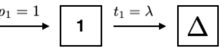
The simplest special case of phase-type distribution is exponential distribution. As-sume that Markov process has one transient state and one absorbing state ∆. Then p={p1}= 1. Let transition rate from the transient state to the absorbing state ist1 :=λ.

Hence, intensity that process stays in the transient state ist1,1 :=−λ. In this case the

time within observed Markov process reaches its absorbing state ∆is exponentially distributed with rate parameterλ. Graphically this process is presented in Figure4.

(26)

Figure 4. The phase-diagram of exponential distribution with rate parameterλ

.

Consider now the classical risk processX(t). If claims’ sizes have phase-type distribu-tion, it is possible to calculate exact ruin probability of observed risk process.

Theorem 3.1. Consider risk processX(t)withc= 1, intensity of Poisson processαand phase-type distributed claims with transition matrixTand initial distributionp. Exact ruin probability ofX(t)can be found as follow

Ψ(u) =p+eT+tp+e,

wherep+=−αpT−1 andeis column vector with all elements equal to one.

Let’s consider one numerical example to illustrate the process of calculation of the ruin probability of a company with phase-type distributed claims.

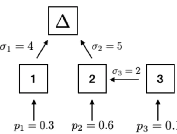
Example 3.1. Suppose that company’s main cash-flows can be described by risk process

X(t)withc= 1and intensity of Poisson distributionα = 3and claims are phase-type distributed with parameters in Figure5. The first moment of this distribution is equal to 0.265. Using the outcome of Theorem3.1let’s find the ruin probability of the company if its initial capital isu.

(27)

Figure 5. Markov chain generating a phase-type distribution

The distribution has three transient states. Hence, the transition matrix T has the following form. T=    −σ1 0 0 0 −σ2 0 0 σ3 −σ3   =    −4 0 0 0 −5 0 0 2 −2   . Therefor the exit rate vectort =−Teis

t=    σ1 σ2 0   =    4 5 0   .

From Figure5we can see that it is possible to reach absorbing state∆directly form states 1 and 2 but not from the state 3.That is why the third element of vectortis equal to zero and the first two elements areσ1andσ2respectively.

Initial distribution of probabilities form which state the Markov process starts p is given by the vector

p=0.3 0.6 0.1

.

Application of Theorem 3.1 requires positive relative safety loadingρ. Let’s check if this condition fulfilled:

ρ= c−αµ

αµ =

1−0.265·3

(28)

Let’s now calculate the vector p+ = −αpT−1. Substitution of the values into the expression ofp+ leads to p+ =−3 0.3 0.6 0.1    −0.25 0 0 0 −0.2 0 0 −0.2 −0.5   = 0.225 0.42 0.15 .

Next we calculate the matrixT+tp+ =:Q(needed in Theorem 3.1):

Q=    −4 0 0 0 −5 0 0 2 −2   +    4 5 0    0.225 0.42 0.15=    −3.1 1.68 0.6 1.125 −2.9 0.75 0 2 −2   

By Theorem3.1we need to find exponential of matrixQu.

Property 3.1. [7]Exponential form ofn×nmatrixQucan be found by the next equation

eQu =φ(u)·φ(0)−1,

whereφ(u)isn×nmatrix which can be presented in block-partitioned form as follow

φ(u) = v1e λ1u_{, v}

2eλ2u . . . , vneλnu !

, (8)

whereλ1, . . . , λ2 are eigenvalues of matrixQandv1, . . . vnare respective right eigen-vectors.

In our case matrixQ(3×3) has three eigenvalues:λ1 =−4.479969,λ2 =−2.885753,

λ3 =−0.634278.

Respective right eigenvectors arev1 =

   0.5593054 −0.6452714 0.5203867   ,v2 =    0.5236681 0.3449783 −0.7789491   ,v3 =    0.5050592 0.4867147 0.7127581   .

By its definition (8) matrixφ(u)has the following form.

φ(u) =    0.5593054e−4.479969u ₀_._5236681_e−2.885753u ₀_._5050592_e−0.634278u −0.6452714e−4.479969u ₀_._3449783_e−2.885753u ₀_._4867147_e−0.634278u 0.5203867e−4.479969u ₋₀_._7789491_e−2.885753u ₀_._7127581_e−0.634278u   .

(29)

Hence,φ−1₍₀₎_is φ−1(0) =    0.7052368 −0.8650708 0.09099351 0.8047468 0.1532572 −0.67489563 0.3645851 0.7990803 0.59899548   .

According to Property3.1, we have

eQ·t =e−4.479969t    0.3944427 −0.4838388 0.05089316 −0.4550691 0.5582055 −0.05871551 0.3669959 −0.4501714 0.04735181   + +e−2.885753t    0.4214202 0.08025592 −0.3534213 0.2776202 0.05287042 −0.2328244 −0.6268568 −0.11937957 0.5257093   + +e−0.634278t    0.1841370 0.4035828 0.3025282 0.1774489 0.3889241 0.2915399 0.2598609 0.5695509 0.4269389   . By Theorem3.1 Ψ(u) =p+eT+tp+e,

which in our case gives

Ψ(u) = 0.004620044·e−4.479969u+ 0.041298121·e−2.885753u+ 0.749081835·e−0.634278u.

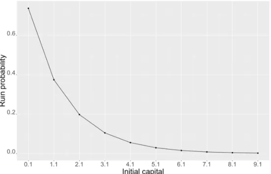
The dependence of the ruin probability on the value of initial capitaluis visualised in Figure6.

(30)

Figure 6. Ruin probability of phase-type distribution for different values of initial capital

As it was shown in Example3.1, evaluating process of exact formula of the ruin prob-ability for a risk process with phase-type distributed claims is not very difficult, but calculations are more complicated in comparison with exponentially distributed claims. Hence, in what follows, for the calculation of the ruin probability self-written R-script is used (Appendix 1).

An important property of phase-type distributions is the formula for the calculation of moments.

Property 3.2. Consider the phase-type distributionBwith the states spaceE, the tran-sition matrixTand the initial distributionp. Thenn-th moment ofB is(−1)nn!pT−ne , whereeisn×1column vector with all elements equal to one.

In the next sections we modify De Vylder’s approximation by replacing exponential distribution with some special cases of phase-type distributions.

(31)

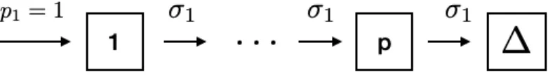
3.2 Erlang distribution

Erlang distributionEp is a special case of Gamma distribution with parameterpmeaning the number of phases. This corresponds to the convolution ofpexponential densities with the same rateσ1. The phase-diagram ofEpis presented in Figure7.

Figure 7. Phase-diagram of Erlang distrbution withpphases

Let’s consider a risk processX(t)with claim distribution for which it is not possible to calculate exact ruin probability. Using the idea of De Vylder’s method we replace initial risk processX(t)with a new risk process Xˆ(t)which has Erlang-distributed claims. Risk process with claims havingEpdistribution (with fixedp) can be described by three parameters: gross premium ratec, intensity of Poisson processα and rate of Erlang distributionσ1. It is sufficient to match the first three moments ofX(t)andXˆ(t)(like in

case of exponential distribution). In other words we need to solve the following system of three equations.        c−α·ζ1 = ˆc−αˆ·E[Z] α·ζ2 = ˆα·E[Z2] α·ζ3 = ˆα·E[Z3] (9)

where Z is the size of claims having Erlang distribution withpphases and rateσ1.

3.2.1 Erlang distribution with two phases

Firstly, assume that claims of the risk processXˆ(t)have Erlang distribution with two phases (E2). The transition matrixTand initial distribution vectorpin case ofE2 have

the following forms:

T= −σ1 σ1 0 −σ1

!

(32)

p=1 0.

The first three moments of Erlang distribution with two phases and rateσ1 can be found

by Property3.2. E[Z] =−1·pT−1e, E[Z2] = 2·pT−2e, E[Z3] =−6·pT−3e, whereeis 1 1 ! .

Substitution ofpandTofE2leads to

E[Z] = 2 σ1 , E[Z2] = 6 σ2 1 , E[Z3] = 24 σ3 1 .

Hence, the system of equations (9) in case ofE2 is the following:

       c−α·ζ1 = ˆc−αˆ· _σ2₁ α·ζ2 = ˆα· _σ62 1 α·ζ3 = ˆα· 24_σ3 1 .

Solving this system of equations analogically to the system (7) in Section 2.1 we get ˆ σ1 = 4ζ2 ζ3 , ˆ α= 8ζ 3 2 3ζ2 3 ·α, ˆ c= 4ζ 2 2 3ζ3 ·α−αζ1+ 1.

We will apply these formulas in Chapter 4. 3.2.2 Erlang distribution with three phases

In the same way, we can estimate parametersˆc,αˆ,σˆ1 of the risk processXˆ(t)in case

(33)

The transition matrixTand initial distributionpfor the Erlang distribution with three phases are the following:

T=    −σ1 σ1 0 0 −σ1 σ1 0 0 −σ1   , p= 1 0 0 .

Substituting this matrices into the outcome of Property3.2the first three moments ofE3

are E[Z] = 3 σ1 , E[Z2] = 12 σ2 1 , E[Z3] = 60 σ3 1 .

Hence, the estimation of parameters of risk processXˆ(t)withE3-distributed claims is

possible to be found from the following system of three equations.        c−α·ζ1 = ˆc−αˆ· _σ3 1 α·ζ2 = ˆα· 12_σ2 1 α·ζ3 = ˆα· 60_σ3 1 . As a result, we get ˆ σ1 = 5ζ2 ζ3 , ˆ α= 25ζ 3 2 12ζ2 3 ·α, ˆ c= 5ζ 2 2 4ζ3 ·α−αζ1+ 1.

(34)

3.3 Hypoexponential distribution with two phases

A generalization of the Erlang distribution is so called hypoexponential distribution. Hypoexponential distribution withpphases is a convolution ofpexponential densities with the intensity rates σ1,. . . ,σp. This is graphically presented in a phase-diagram (Figure8)

Figure 8. Phase-diagram of hypoexponential distribution withpphases

The number of parameters describing risk process Xˆ(t)with hypoexponentially dis-tributed claims varies depending on the number of phases of the distribution. For example, if there is only one phase,Xˆ(t)can be described by three parameters, hence in this case hypoexponential distribution turns into simple exponential distribution. But if the number of states is equal to two, Xˆ(t) is described by four parameters: gross premium rateˆc, intensity of Poisson processαˆ, transition intensities from state "1" to state "2" and from state "2" to absorbing state, σˆ1 and σˆ2, respectively. Further we

consider a risk processXˆ(t)with two-phases hypoexponentially distributed claims. Suppose now that the risk process X(t) has a claim distribution, for which there is no exact formula for ruin probability. Analogically to previous section we use the idea of De Vylder’s method to replace initial risk processX(t)with a new risk processXˆ(t) which has two-phases hypoexponentially distributed claims. As it was mentioned above,

ˆ

X(t)can be described by four parameters. So in this case, it is necessary to match the first four moments ofX(t)andXˆ(t)to find the estimationXˆ(t)parameters.

The first three moments of classical risk process are evaluated in Section 2.1. The fourth moment can be found analogically by Property2.1( adding fourth term into Taylor series ofe−ivZk_).

E[X(t)4] = 2αζ4t+ (c−αζ1)4t4 + 6α(c−αζ1)2ζ2t3−4α(c−αζ1)ζ3t2+ 3α2ζ22t 2

(35)

Hence, to match the first four moments ofX(t)andXˆ(t), it is sufficient to solve the following system of equations

             c−α·ζ1 = ˆc−αˆ·E(Z) α·ζ2 = ˆα·E(Z2) α·ζ3 = ˆα·E(Z3) α·ζ4 = ˆα·E(Z4) . (10)

The transition matrixTand initial distributionpof hypoexponential distribution with two phases are the following

T= −σ1 σ1 0 −σ2 ! , p=1 0 .

By Property3.2the first four moments of this distribution are

E(Z) = 1 σ1 + 1 σ2 , E(Z2) = 2· 1 σ1σ2 + 1 σ2 1 + 1 σ2 2 , E(Z3) = 6· 1 σ2 1σ2 + 1 σ1σ22 + 1 σ3 1 + 1 σ3 2 , E(Z4) = 24· 1 σ3 1σ2 + 1 σ2 1σ22 + 1 σ1σ32 + 1 σ4 1 + 1 σ4 2 .

Substitution of the moments of hypoexponential distribution into the system (10) leads to                c−α·ζ1 = ˆc−αˆ· 1 σ1 + 1 σ2 α·ζ2 = 2·αˆ· 1 σ1σ2 + 1 σ2 1 +_σ12 2 α·ζ3 = 6·αˆ· 1 σ12σ2 + 1 σ1σ22 + 1 σ13 + 1 σ23 α·ζ4 = 24·αˆ· 1 σ3 1σ2 + 1 σ2 1σ22 + 1 σ1σ32 + 1 σ4 1 + 1 σ4 2 .

It is not mathematically easy to solve this system manually. So, to estimate parameters ofXˆ(t)Maxima software was used (Appendix 2). The relations obtained between the parameters ofX(t)andXˆ(t)are too long and complex, thus they are not presented in the text. We will apply obtained formulas in Chapter 4.

(36)

3.4 Hyperexponetial distribution with two phases

Another popular case of phase-type distributions is hyperexponential distributionHp with p phases. It is defined as a mixture of p exponential distributions with rates

σ1, σ2, . . . , σp. The phase-diagram ofHpis presented in Figure9. Weightsp1, . . . , ppof hyperexponential distributionHp are such that

Pp

k=1pk = 1. In the framework of this thesis we consider two-phases hyperexponential distribution.

Figure 9. Phase-diagram of hyperexponential distrbution withpphases

Analogically to the previous section, let us assume that it is not possible to calculate exact ruin probability for the risk processX(t). Our aim is to replaceX(t)with a suitable risk processXˆ(t)which has two-phases hyperexponenntially distributed claims. Such risk process can be described by six parameters: weightspˆ1andpˆ2, transition intensitiesσˆ1

andσˆ2, gross premium ratecˆand intensity of Poisson distributionαˆ. Since the sum of

the weights of hyperexponential distribution is always equal to one, it is sufficient to know only one of the weights. For example, if estimation of the first weight ispˆ1, then

estimation of the second one ispˆ2 = 1−pˆ1. Hence, it is sufficient to match the first five

moments ofX(t)andXˆ(t).

The fifth moment of classical risk process is evaluated by Property2.1( adding fifth term into Taylor series ofe−ivZk_).

E[X(t)5] = (c−αζ1)5t5+ 10a(c−αζ1)3ζ2t4−10α(c−αζ1)2ζ3t3

+ 15α2(c−αζ1)ζ22t 3

(37)

Hence, to match the first five moments of X(t) and Xˆ(t) it is needed to solve the following system of equations

                   c−α·ζ1 = ˆc−αˆ·E(Z) α·ζ2 = ˆα·E(Z2) α·ζ3 = ˆα·E(Z3) α·ζ4 = ˆα·E(Z4) α·ζ5 = ˆα·E(Z5) (11)

The transition matrixTand initial distributionpin case ofH2distributions are

T= −σ1 0 0 −σ2 ! , p=p1 1−p1 .

By Property3.2the first five moments of hyperexponential distribution with two phases are the following:

E(Z) = p1 σ1 +1−p1 σ2 , E(Z2) = 2· p1 σ2 1 + 1−p1 σ2 2 , E(Z3) = 6· p1 σ3 1 + 1−p1 σ3 2 , E(Z4) = 24· p1 σ4 1 +1−p1 σ4 2 , E(Z5) = 120· p1 σ5 1 +1−p1 σ5 2 .

Substitution of the moments of hyperexponential distribution into the system (11) leads to                      c−α·ζ1 = ˆc−αˆ· p1 σ1 + 1−p1 σ2 α·ζ2 = 2·αˆ· p1 σ2 1 + 1−p1 σ2 2 α·ζ3 = 6·αˆ· p1 σ3 1 + 1−p1 σ3 2 α·ζ4 = 24·αˆ· p1 σ4 1 + 1−p1 σ4 2 α·ζ5 = 120·αˆ· p1 σ5 1 +1−p1 σ5 2 .

(38)

This system was solved using Maxima software (Appendix 2). The relations obtained between the parameters ofX(t)andXˆ(t)are too long and complex, thus they are not presented in the text. We will apply obtained formulas in Chapter 4.

3.5 Coxian distributions

Coxian distribution is very popular class of phase-type distributions in applied literature. This distribution has the following form of the phase-diagram (Figure10).

Figure 10. Phase-diagram of Coxian distrbution withpphases

Coxian distribution is a generalization of hypoexpoential distribution. Instead of only being able to reach the absorbing state from the final phasepit can be reached from any phase. Parameterst1, . . . , tp−1 ∈[0,1]. If allti are equal to one, then Coxian distribution is exactly hypoexponential distribution.

Analogically to the previous sections we calculate the ruin probability for risk pro-cess X(t) by replacing initial risk process X(t) with a new risk process Xˆ(t) with Coxian distribution of claims. In this section we will consider two cases of Coxian distribution.

3.5.1 Simplified two-phases Coxian distribution

First of all, let’s assume that the risk processXˆ(t)has two-phases Coxian distibution of claims, such thatσ1 =σ2, i.e. its phase-diagam has the form presented in Figure11.

(39)

Figure 11. Phase-diagram of simplified Coxian distribution with two phases

This risk process can be described by four parameeters: transition intensityσˆ1 andt1,

gross premium rateˆc, intensity of Poisson distributionαˆ. Hence, in order to estimate all unknown parameters of this special case of Coxian distribution it is needed to match the first four moments ofX(t)andXˆ(t).

The transition matrixTand initial distributionpin case of considered case of Coxian distributions are the following:

T= −σ1 σ1·t1 0 −σ1 ! , p=1 0 .

By Property3.2the first four moments of simplified Coxian distribution with two phases are the following:

E(Z) = t1+ 1 σ1 , E(Z2) = 2· 2t1+ 1 σ2 1 , E(Z3) = 6· 3t1+ 1 σ3 1 , E(Z4) = 24· 4t1 + 1 σ4 1 .

(40)

Hence, in order to match the first four moments of initial risk processX(t)and new risk processXˆ(t)with Coxian distribution of claim, parameters ofXˆ(t)must satisfy the following system of equations:

               c−α·ζ1 = ˆc−αˆ· t1+1 σ1 α·ζ2 = 2 ˆα· 2t1+1 σ2 1 α·ζ3 = 6 ˆα· 3t1+1 σ3 1 α·ζ4 = 24 ˆα· 4t1+1 σ41 . (12)

This system has two solutions: ˆ t1 = 3− 9ζ2ζ4 4ζ2 3 ±q1− 3ζ2ζ4 4ζ2 3 27ζ2ζ4 4ζ2 3 −8 , ˆ σ1 = 4ζ3(1 + 4ˆt1) ζ4(1 + 3ˆt1) , ˆ α= ζ3σˆ 3 1 6(1 + 3ˆt1) ·α, ˆ c= 1−αζ1+ ˆα· _ˆ t1+ 1 ˆ σ1 .

We will apply these formulas in Chapter 4.

3.5.2 General two-phases Coxian distribution

Now let us assume that claims of the risk processXˆ(t)have general Coxian distribution with two phases i.e. there is no assumption that σ1 = σ2. In this case Xˆ(t)has five

unknown parameters: σˆ1,σˆ2,ˆt1,ˆc,αˆ. Hence, it is needed to match the first five moments

ofX(t)andXˆ(t)to find the estimations of unknown parameters.

The transition matrix Tand initial distributionpfor general Coxian distributions are defined as follow T= −σ1 σ1·t1 0 −σ2 ! , p=1 0 .

(41)

By Property3.2the first four moments of simplified Coxian distribution with two phases are the following:

E(Z) = t1 σ2 + 1 σ1 , E(Z2) = 2· t1 σ1σ2 + t1 σ2 2 + 1 σ2 1 , E(Z3) = 6· t1 σ2 1σ2 + t1 σ1σ22 + t1 σ3 2 + 1 σ3 1 , E(Z4) = 24· t1 σ3 1σ2 + t1 σ2 1σ22 + t1 σ1σ23 + t1 σ4 2 + 1 σ4 1 , E(Z4) = 120· t1 σ4 1σ2 + t1 σ3 1σ22 + t1 σ2 1σ23 + t1 σ1σ24 + t1 σ5 2 + 1 σ5 1 .

The estimation of the parameters of Xˆ(t)can be found from the following system of equations.                      c−α·ζ1 = ˆc−αˆ· t1 σ2 + 1 σ1 α·ζ2 = 2·αˆ· t1 σ1σ2 + t1 σ2 2 +_σ12 1 α·ζ3 = 6·αˆ· t1 σ2 1σ2 + t1 σ1σ22 + t1 σ3 2 + 1 σ3 1 α·ζ4 = 24·αˆ· t1 σ3 1σ2 + t1 σ2 1σ22 + t1 σ1σ23 + t1 σ4 2 +_σ14 1 α·ζ5 = 120·αˆ· t1 σ4 1σ2 + t1 σ3 1σ22 + t1 σ2 1σ23 + t1 σ1σ42 + t1 σ5 2 + 1 σ5 1

This system of equations was solved using Maxima software (Appendix 2). We will apply obtained formulas in Chapter 4.

(42)

4 Numerical comparison of De Vylder’s approximation

and phase-type approximations

The goal of this chapter is numerical comparison of the accuracy of ruin probability’s approximations based on De Vylder’s method and phase-type distributions considered in the previous chapter. In Section 2.2 De Vylder’s approximation was applied on three examples: Gamma distribution (Example 2.1), mixed exponential distribution (Example 2.2) and lognormal distribution (Example 2.3). In this chapter we calculate ruin probabil-ities for the same examples using phase-type approximations and compare relative errors of all methods.

Sometimes claims of risk processes have complicated, high-order phase-type distri-butions with many states. It is not technically simple to calculate the ruin probability in such cases, even when exact formula is known. Hence, we got an idea to check if it is possible to estimate accurately the ruin probability in such cases using claims with a simple, low-order phase-type distributions. In order to research this question, one more numerical example is considered.

4.1 Gamma distribution

Consider the risk processX(t)described in Example 2.1. It means claims are having Gamma distribution with parameters α0 = ₁₀₀1 andβ0 = ₁₀₀1 , intensity of the Poisson processα = 10₁₁, relative safety loadingρ= 5%and gross premium ratecis assumed to be equal to 1.

As it was shown in Section 2.2 (Table 1), de Vylder’s approximation works well in case of claims having Gamma distribution. The summary of absolute relative errors for all considered methods is presented in Figure13. Here and in the next sections the following notations are used:

• De Vylder - De Vylder’s approximation

• Erlang2 - approximation based on two-phases Erlang distribution, described in Section 3.2.1.

• Erlang3 - approximation based on three-phases Erlang distribution, described in Section 3.2.2.

(43)

• Hypo2 - approximation based on two-phases hypoexpontial distribution, described in Section 3.3.

• Hyper2 - approximation based on two-phases hyperexponential distribution, de-scribed in Section 3.4.

• Coxian1 - approximation based on simplified two-phases Coxian distribution, described in Section 3.5.1.

• Coxian2 - approximation based on general two-phases Coxian distribution, de-scribed in Section 3.5.2.

Table 4. Absolute relative errors (Gamma distributed claims)

In case of Gamma distributed claims the most accurate approximation is given by hyperexponential (Hyper2) and general Coxian distributions (Coxian2). As can be seen from Table 4, these approximations gives exactly the same absolute relative errors.

(44)

Figure 12. Estimation of parameters of general Coxian distribution

Figure 13. Estimation of parameters of hyperexponential distribution

Estimated rate parameters of these two distributions are equal (σ1Coxian2 = σ2Hyper2 and

σ2Coxian2 =σ1Hyper2). As a result, Coxian2 and Hyper2 give exactly the same formula of the ruin probability in case of Gamma distributed claims.

Ψ(u)H2= Ψ(u)Coxian2= 0.01970989e−0.019107186u+ 0.87942839e−0.001745007u

There is a clear theoretical reason for such a coincidence. Namely, it is known phase-type distribution that has no cycles in the phase-diagram can equivalently be represented as a Coxian phase-type distribution.[11] The reader can notice the same phenomena in the following examples too.

(45)

Simplified Coxian (Coxian1) and hypoexpontial (Hypo2) distributions give very ac-curate results too. Absolute relative errors are slight greater than in case of Hyper2 and general Coxian2 but still smaller than errors of De Vylder’s approximations for most of the values of initial capitalu. Erlang distributions with two (Erlang2) and three (Erlang3) phases give the worst approximations compare to other methods, but still work well and relative errors do not exceed1%. The plot of relative errors for all seven approximations is presented in Figure14

Figure 14. Relative error of ruin probabilities of approximations (Gamma distribution)

4.2 Mixed exponential distribution

Assume now that the sizes of the claims of the risk processX(t)have mixed exponential (hyperexponenial) distribution with the distribution functionF(z).

F(z) = 1−0.0039793·e−0.014631z−0.1078392·e−0.190206z−0.8881815·e−5.514588z.

We considerρ= 5%;10%;15%;20%;25%;30%;100%. Gross premium ratecis taken to be equal to one.

(46)

Table 5. Absolute relative errors (Mixed exponentially distributed claims)

The results of approximations are analogical to the previous example with Gamma distribution. The smallest absolute relative errors are obtained by approximations with hyperexponential and general Coxian distributions. Note that these two approximations give almost perfect result (errors do not exceed0.083%). In this example such result is not surprising. Initial distribution of claims is hyperexponential distribution with three phases. Moreover the weight of the first state is small enough (w1 = 0.0039793). Hence

distribution of claims ofX(t)is close to two-phases hyperexponential distribution. That is why Hyper2 and hence Coxian2 give almost perfect approximation.

(47)

Figure 15. Relative errors for different values ofρ(u= 10).

Let’s compare relative errors of the approximations depending on the values of the relative safety loading. From Figure15it is seen that Hyper2 and Coxian2 approximations are stable and give almost perfect approximation independently on ρ, but for all other methods there is the same trend in case ofρ∈[5%,30%]. All methods underestimate the ruin probability and increasing the value of relative safety loading absolute relative errors of approximations are logarithmically increasing. Comparing relative errors in case ofρ = 30%andρ = 100%, we can see that Coxian1 and Hypo2 approximations give a bit more exact estimation of ruin probability for higher value of relative safety loading, while errors of others approximations continue increasing.

4.3 Lognormal distribution

As it was shown in Example 2.3(Section 3.2), De Vylder’s method can not precisely estimate ruin probability of a risk process if claims have lognormal distribution. Consider the same risk processX(t)with lognormally distributed claims (σ2

L = 3.24,µL =−1.62) and compare the accuracy of phase-type approximations.

(48)

Table 6. Absolute relative errors (Lognormal distribution)

From Table6we can see, that absolute relative errors are big in most of the cases. Risk process with any phase-type distribution of claims has exponentially decreasing ruin probability. Hence, it is not surprising that considered methods can not estimate ruin probability in case of lognormally distributed claims. Hence, relatively good estimation of the ruin probability, for example, in case ofρ= 25%andu= 100can be considered as accidental.

Interesting is the fact that in case of Hypo2 and Coxian1 methods estimation of pa-rameters do not give an adequate result. For example, one of the rate papa-rameters of two phases hypoexponential distribution is complex number with negative real part (ˆσ2 = −6.419022·10−4 + 8.972437·10−4i). Complex number as an estimation of

parameters of a risk process Xˆ(t)has been already met in case of hypoexponentialy distributed claims in previous examples but the real part of the number was positive and as result, it does not affect the estimation of ruin probability. In this example negativity of the real part of parameter estimation causes non-adequate ruin probability formula (probability is increasing if initial capital increases).

Two-phases hypoexponential and simplified Coxian distributions are, of course, gen-eral cases of two-phases Erlang distribution and that is why the question arises: why Hypo2 and Coxian1 can not adequately estimate the parameters if Erlang2 can handle it. The nature of the problem is based on the number of restrictions in case of each claim

(49)

distribution. As it was mentioned before risk processXˆ(t)with Erlang distribution of claims has three parameters. Hence, to estimate them it is needed to match the first three moments of initial risk process andXˆ(t). In case of two-phases hypoexponential and simplified Coxian distributions there are four and five parameters respectively. Hence, because of greater number of restrictions it is not mathematically possible to obtain same result as in case of Erlang2.

4.4 Phase-type distribution with many states

Assume now that claims of a risk processX(t)has phase-type distribution with many states. The goal of this section is to study if it possible to accurately estimate the ruin probability ofX(t)using approximations considered in Chapter 3.

Example 4.1.

Let distribution of claims of a risk processX(t)is phase-type with ten states. Phase-diagram of this distribution is presented in Figure16

(50)

Assume that p1 = 0.6; p2 = 0.4; σ1,3 = 1.3; σ2,4 = 2.4; σ3,5 = 3.5; σ3,6 = 3.6;

σ4,6 = 4.6; t4,6 = 0.2; σ5,7 = 1.7; σ6,8 = 3.8; σ6,9 = 2.9; σ7,10 = 1.10; σ8 = 0.8;

σ9 = 0.9;σ10= 0.10. Then we can estimate ruin probabilities of the risk processX(t)

by considered in the previous chapter methods.

Table 7. Absolute relative errors (Phase-type distribution with many states, example 4.1)

As we can see from Table7, the hyperexponential and general Coxian distributions with only two phases perfectly fit the high-order phase-type distribution for all values of initial capital and relative safety loading. Hypo2 is also very accurate approximation but it works worse in case of small initial capital when ruin probability is higher. De Vylder’s approximation, Erlang2, Erlang3 and Coxian1 give really poor results in case of small ruin probability (highρand bigu). To conclude, we can say that all approximations give relatively accurate estimations of the ruin probability ofX(t). This depends, of course, on the values of parameters of claim distribution.

(51)

Example 4.2.

Consider now same type of claim distribution, but with another values of parameters. Assume that p1 = 0.6; p2 = 0.4; t4,6 = 0.2 andσ1,3 = σ2,4 = σ3,5 = σ3,6 = σ4,6 =

σ5,7 =σ6,8 =σ6,9 =σ7,10=σ8 =σ9 =σ10= 1.

In this case Hypo2 approxiamtion can not adequately estimate parameters and give incorrect formula of the ruin probability (probability is increasing if initial capital in-creases). Hence, the only approximations which work correctly in this case are De Vylder’s approximation, Erlang2, Erlang3, Hyper2, Coxian1 and Coxian2.

Table 8. Absolute relative errors (Phase-type distribution with many states, example 4.2)

From Table8we can see that working approximation methods give very accurate results in most of cases. Hyper2 and Coxian2 with only two phases perfectly fit the high-order phase-type distribution for all values of initial capital and relative safety loading. Since all transition rates of this phase-type distribution are equal, Erlang3 also returns very

(52)

accurate estimation of the ruin probability. The worst approximation (in comparison with other approximations) is De Vylder’s method. Note that in case of highρand bigu

(ruin probability is small in this case) De Vylder’s method returns very poor result. For example, ifρ= 100%andc= 200absolute relative error is274,33%.

To conclude, approximation based on low-order phase-type distribution can accurately estimate the ruin probabilities of a risk process, in case if its claims have complicated, high-order phase-type distributions with many states. De Vylder’s approximation returns an accurate estimation of the ruin probability based on considered examples, but absolute relative errors of this method are several times bigger than errors of Hyper2 and Coxian2.

(53)

Conclusion

The main goal of the thesis was to find a method of approximation of the ruin probabil-ity that is more accurate than famous De Vylder’s method but at the same time is not technically too complicated. In the framework of this thesis six approximations were considered based on phase-type distributions for calculation of the ruin probability. Ac-curacy of each approximation were compared based on four examples of risk processes with different distributions of claims.

In this thesis we examined mostly approximations based on phase-type distributions with two phases. The number of parameters describing a risk process with Coxian, hypoexponential or hyperexponential distribution of claims depends on the number of phases. Even in case of two phases these approximations need to solve systems of four or five equations which are much more difficult than in case of De Vylder’s approximation. Hence, the number of phases was limited by two for these distributions. Three-phases case was considered for Erlang distribution, since the number of unknown parameters describing a risk process with Erlang distribution is always three and does not depend on the numbers of phases.

Comparison of absolute relative errors of ruin probability’s estimations showed that hyperexponential and general Coxian distributions give the most accurate results based on examples of risk process with Gamma and mixed exponentially distributed claims. In these cases named approximations fit the ruin probability perfectly and relative errors are negligible. The biggest errors are seen if approximation is based on two- or three-phases Erlang distribution. Their absolute relative errors are even higher than in case of De Vylder’s method. Moreover, increasing of the number of phases of Erlang distributions worsens the result.

Risk processes with lognormally distributed claims are badly fitted by De Vylder’s approximation. It is well understood since in lognormal case the ruin probability follows the asymptotic which significantly differes from exponential asymptotic. In this thesis it was shown that phase-type distributions can not correctly describe it too, since they return exponentially decreasing ruin probability.

To conclude, our new approximation methods based on simple phase-type distribu-tions (such as hyperexponential and general Coxian) almost always give more accurate

(54)

ruin probabilities than well-known De Vylder’s method. At the same time, the price for the increased accuracy is only minimal, since ruin probabilities for phase-type distributed claims can still be calculated via explicit formulas, without any time consuming iterations.

(55)

References

[1]Pärna, K. (2018). Risk Theory. Lecture notes.

[2]Grandell, J. (1991). Aspects of Risk Theory. New-York: Springer-Verlag.

[3]Albrecher, H. and Asmussen, S. (2010). Ruin Probabilities. Published by World Scientific Publishing Co. Pte. Ltd. (second edition).

[4]Pärna, K. (2018). Stochastic Models. Lecture notes.

[5]Käärik, M. (2019). Non-life Insurance Mathematics. Lecture notes.

[6]Cramer, H. (1946). Mathematical Methods of Statistics. Bombay: Asia Publishing House

[7]Mattuck A., Miller H., Orloff J. and Lewis J. (2011) Differential Equations. Mas-sachusetts Institute of Technology: MIT OpenCourseWare, https://ocw.mit.edu.

[8]Ushakov, N. G. (1999) Selected topics in characteristic functions. Published by De Gruyter.

[9]Panchenko, D. (2006) Statistics for Applications. Massachusetts Institute of Technol-ogy: MIT OpenCourseWare, https://ocw.mit.edu.

[10]Papadopolous, H. T., Heavey, C. and Browne, J. (1993). Queueing Theory in Manu-facturing Systems Analysis and Design. London: Chapman & Hall.

[11] Dehon M. and Latouche G. (1982) A Geometric Interpretation of the Relations between the Exponential and Generalized Erlang Distributions. Advances in Applied Probability Vol. 14, No. 4.

[12] Anderson, W. J. (1991). Continuous-Time Markov Chains: An Applications-Oriented Approach. New-York: Springer-Verlag