Subspace clustering for complex data

(1)

Subspace Clustering

for Complex Data

Von der Fakult¨at f¨ur Mathematik, Informatik und Naturwissenschaften der RWTH Aachen University zur Erlangung des akademischen Grades

eines Doktors der Naturwissenschaften genehmigte Dissertation

vorgelegt von Diplom-Informatiker Stephan G¨unnemann

aus Meppen

Berichter: Univ.-Prof. Dr. rer. nat. Thomas Seidl Prof. Dr. sc. techn. Martin Ester Tag der m¨undlichen Pr¨ufung: 15.03.2012

Diese Dissertation ist auf den Internetseiten der Hochschulbibliothek online verf¨ugbar.

(2)

(3)

Subspace Mining on Vector Data

17

2 Relevant Subspace Clustering 19 2.1 Motivation and Comparison with Related Work . . . 20

2.2 Relevant Subspace Clustering . . . 22

2.3 The RESCU Algorithm . . . 36

2.4 Experimental Analysis . . . 40

2.5 Conclusion . . . 46

3 Detection of Orthogonal Concepts 47 3.1 Motivation . . . 48

3.2 Comparison with Related Work . . . 50

3.3 Orthogonal Concepts in Subspaces . . . 52

3.4 The OSCLU Algorithm . . . 61

4 Multi-View Subspace Clustering via Multiple Mixture Models 73 4.1 Motivation and Comparison with Related Work . . . 74

4.2 Formal Description of the Model . . . 77

4.3 The MVGen Algorithm . . . 84 i

(4)

ii CONTENTS

5 Subspace Correlation Clustering 103 5.1 Motivation . . . 103

5.3 Subspace Correlation Clustering . . . 109

5.4 The SSCC Algorithm . . . 117

II

Subspace Mining on Imperfect Data

131

6 Imperfect Data: Introduction 133 6.1 Types of Imperfect Information . . . 133

6.2 Data Cleansing . . . 135

7 Subspace Clustering for Incomplete Data 137 7.1 Motivation and Comparison with Related Work . . . 138

7.2 Fault Tolerant Subspace Clustering Model . . . 140

7.3 Instantiation and FTSC Algorithm . . . 151

8 Subspace Clustering for Uncertain Data 161 8.1 Motivation . . . 161

8.3 Subspace Clustering for Uncertain Data . . . 165

8.4 Algorithmic Properties . . . 177

III

Subspace Mining on Heterogeneous Data

189

9 Heterogeneous Data: Introduction 191 9.1 Data Heterogeneity . . . 191

(5)

CONTENTS iii

9.2 Mining Diversity . . . 192

10 A Synthesis of Subspace Clustering and Dense Subgraph Mining 195 10.1 Motivation . . . 196

10.3 An Integrated Clustering Model . . . 201

10.4 The GAMER Algorithm . . . 211

11 Efficient Mining of Combined Subspace and Subgraph Clusters 243 11.1 Motivation . . . 243

11.3 Quality-Optimal Clustering . . . 246

11.4 The EDCAR Algorithm . . . 255

12 Density-Based Subspace Clustering for Graph Data 269 12.1 Motivation and Comparison with Related Work . . . 269

12.2 A Density-Based Clustering Model for Combined Data . . . 272

12.3 The DB-CSC Algorithm . . . 282

IV

Summary

299

13 Conclusion and Future Work 301 13.1 Conclusion . . . 301

13.2 Future Work . . . 304

Appendices

I

Bibliography III

List of Publications XXIII

(6)

(7)

Abstract

The increasing potential of storage technologies and information systems has opened the possibility to conveniently and affordably gather large amounts of complex data. Going beyond simple descriptions of objects by some few character-istics, such data sources range from high dimensional vector spaces over imperfect data containing errors to network data describing relations between the objects. Data Mining is the task of extracting previously unknown and useful patterns from such data sources by using automatic or semi-automatic algorithms. In this thesis, we focus on the mining task ofclustering, which aims at grouping similar objects while separating dissimilar ones.

Since in today’s applications usually many characteristics for each object are recorded, one cannot expect to find similar objects by considering all attributes together. In contrast, valuable clusters are hidden in subspace projections of the data. As a general solution to this problem, the paradigm of subspace clustering has been introduced, which aims at automatically determining for each group of objects a set of relevant attributes these objects are similar in.

In this thesis, we introduce novel methods for effective subspace clustering on various types of complex data. Our methods tackle major open challenges for clustering in subspace projections. We study the problem of redundancy in subspace clustering results and propose models whose solutions contain only non-redundant and, thus, valuable clusters. Since different subspace projections repre-sent different views on the data, often several groupings of the objects are reason-able. Thus, we propose techniques that are not restricted to a single partitioning of the objects but that enable the detection of multiple clustering solutions. Be-sides tackling these challenges of subspace clustering for the case of vector data, we study the task of subspace clustering on two further data types: imperfect data and network data in combination with vector data. We propose integrated mining techniques directly handling errors in the data and simultaneously mining differ-ent information sources. In thorough experimdiffer-ents, we demonstrate the strengths of our novel clustering approaches. Overall, for the first time, meaningful subspace clustering results can be obtained for these types of complex data.

(8)

(9)

Zusammenfassung

Das gestiegene Potential von Speichertechnologien und Informationssystemen hat die Möglichkeit eröffnet, kostengünstig große Mengen an komplexen Daten zu sammeln. Neben einfachen Beschreibungen von Objekten durch einige wenige Attribute reichen diese Datenquellen von hochdimensionalen Vektorräumen über unvollkommene Daten hin zu Netzwerkdaten. Die Aufgabe des Data Mining ist es, mit Hilfe von automatischen oder semi-automatischen Algorithmen aus diesen Datenquellen bislang unbekannte und nützliche Muster zu extrahieren. In dieser Arbeit betrachten wir die Aufgabe desClusterings, die darauf abzielt Gruppen von ¨

ahnlichen Objekten zu bilden und gleichzeitig unähnliche Objekte zu trennen. Da in heutigen Anwendungen häufig sehr viele Eigenschaften für jedes Objekt gespeichert werden, ist nicht zu erwarten, dass Objekte existieren, die bei Betrach-tung der Gesamtheit aller Eigenschaften ähnlich zueinander sind. Vielmehr wer-den sinnvolle Gruppen nur in Teilräumen des Datenraums gefunden. Als Lösung für dieses Problem wurde das Paradigma desSubspace Clusteringseingeführt, wel-ches automatisch für jede Gruppe von Objekten eine zugehörige Menge relevanter Attribute identifiziert, in welchen die Objekte ähnlich zueinander sind.

In dieser Arbeit führen wir neue Methoden für ein effektives Subspace Cluster-ing auf verschiedenen Typen von komplexen Daten ein. Wir untersuchen das Pro-blem der Redundanz in Subspace Clustering-Ergebnissen und schlagen neue Mo-delle zur Vermeidung dieser Redundanz vor. Da jeder Teilraum eine andere Sicht auf die Daten liefert, können häufig mehrere sinnvolle Gruppierungen der Objekte gefunden werden. Daher führen wir Techniken ein, die nicht auf eine einzige Partitionierung der Objekte eingeschränkt sind sondern mehrere unterschiedliche Gruppierungen finden können. Neben der Lösung dieser Herausforderungen für das Subspace Clustering von vektoriell beschriebenen Daten analysieren wir ferner das Subspace Clustering auf unvollkommenen Daten sowie auf einer Kombina-tion von Netzwerkdaten mit vektoriellen Daten. Wir schlagen integrierte Ana-lysetechniken vor, welche mit Fehlern in den Daten umgehen können und ver-schiedene Datenquellen simultan analysieren. In experimentellen Untersuchun-gen zeiUntersuchun-gen wir die Stärken der neu entwickelten Clustering-Methoden. Insgesamt ermöglichen wir erstmalig die Bestimmung eines sinnvollen Subspace Clustering für diese komplexen Daten.

(10)

(11)

Chapter 1

Overview of Thesis

1.1

Introduction

The increasing potential of storage technologies and information systems over the last decades has opened the possibility to conveniently and affordably gather large amounts of complex data. Going beyond simple descriptions of objects by some few characteristics, such data sources range from high dimensional vector spaces over imperfect data containing errors to network data describing relations be-tween the objects. While storing these data is common, their analysis is challeng-ing: the human capabilities of a manual analysis are quickly exhausted consid-ering the mere size of the data. Thus, automatic techniques supporting the user in the process of knowledge extraction are required to gain a benefit from the collected data.

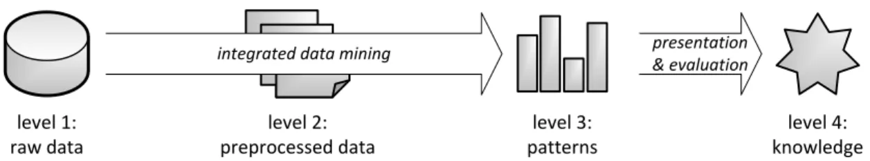
The concept of Knowledge Discovery in Databases (KDD) [HK01] has been evolved as a possible solution for the above challenge and it is coherently de-scribed by a multilevel process the user has to follow (cf. Figure 1.1). Given the raw data, which is rarely perfect since, e.g., missing entries, inconsistencies, or uncertain values are prevalent during the data acquisition phase, the KDD process starts with a preprocessing step to clean the data. This step is often referred to data cleansing and tries to increase the data quality to support the subsequent data mining step. The goal of data mining, as the key component of the KDD process, is to extract previously unknown and useful patterns from the data using automatic or semi-automatic algorithms. Finally, the KDD process concludes with the

(12)

6 Overview of Thesis level 1: raw data level 2: preprocessed data level 3: patterns level 4: knowledge

preprocessing data mining presentation & evaluation

level 1:

raw data

level 2:

preprocessed data

level 3:

patterns

preprocessing data mining prese

& eva

Figure 1.1: Knowledge Discovery in Databases (KDD) process

sentation and evaluation of the detected patterns, enabling the user to understand and interpret the results.

In this thesis we focus on the development of novel models and algorithms for the central step of the KDD process: data mining. Out of the several mining tasks that exist in the literature, this work centers on the important method of clus-tering, which aims at grouping similar objects while separating dissimilar ones. Clustering, as an unsupervised learning task, analyses data without given labels but automatically reveals the hidden structure of the data by its aggregations. For today’s data, however, it is known that traditional clustering methods fail to de-tect meaningful patterns. The problem originates from the fact that traditional clustering approaches consider the full space to measure the similarity between objects, i.e. all characteristics of the objects are taken into account. While collect-ing more and more characteristics, however, it is very unlikely that two objects are similar with respect to the full space and often some dimensions are not rele-vant for clustering. A continuative aspect is the decreasing discrimination power of distance functions with increasing dimensionality of the data space due to the ”curse of dimensionality” [BGRS99]. The distances between objects grow more and more alike, thus all objects seem equally similar based on their attribute val-ues. Since clusters are strongly obfuscated by irrelevant dimensions and distances are not discriminable any more, searches in the full space are futile or lead to very questionable clustering results.

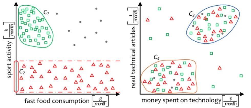
Global dimensionality reduction techniques, e.g., based on Principal Compo-nent Analysis (PCA [Jol02]), try to mitigate these effects, but they do not provide a solution to this problem. Since they reduce all objects to a single projection, they cannot detect clusters with locally relevant dimensions. In complex data sets, however, different groups of objects may have different relevant dimensions. In Figure 1.2, the objects depicted as rectangles are similar in a 2-dimensional

(13)

sub-1.1. Introduction 7 sport activity h mo nt h read technica l articles 1 month

fast food consumption _monthg money spent on technology $

month

C1

C2

C3

C4

Figure 1.2: Exemplary subspace clustering of a 4-dimensional database

space, while the objects depicted as triangles show only similar values in a single dimension.

As a general solution to this problem, the paradigm of subspace clustering [PHL04, KKZ09] has been introduced. Subspace clustering detects clusters in arbi-trary subspace projections of the data by automatically determining for each group of objects a set of relevant dimensions these objects are similar in. Thus, in Figure 1.2 the objects grouped in cluster C1 would correspond to a subspace cluster in

subspace {fast food consumption, sport activity}, while the cluster C2 is only

lo-cated in subspace{sport activity}. Since different subspaces may lead to different groupings, each object can naturally belong to multiple clusters as illustrated in Figure 1.2 (right). The subspaces individually assigned to each group provide the reasoning why such multiple solutions are meaningful. Thus, in the example of Figure 1.2, each of the four clusters{C1, . . . , C4}is useful and should be provided

to the user.

In this thesis we introduce novel methods for effective subspace clustering on complex data including high-dimensional vector spaces, imperfect data, and het-erogeneous data. Such clustering methods are beneficial for various applications: In customer and social network analysis, persons can be grouped according to their similarity based on some product relevant attributes. In bioinformatics, groups of genes that show similar expression levels in a subset of experimental medical treatments can be identified. In sensor network analysis, different environmen-tal events can be described by similarly behaving sensors with respect to specific measured variables. For all of these domains objects are characterized by many attributes, while the clusters appear only in subspace projections of the data.

(14)

8 Overview of Thesis

1.2

Subspace Clustering for Complex Data

In the previous section we introduced the basic objective of subspace clustering. Though, achieving this objective, especially for today’s complex data, is subject to several challenges, which we will discuss in this section. These challenges affect different levels of the KDD process and in total they support the demand for novel, effective subspace clustering models as developed in this thesis.

Challenges for Subspace Clustering on Vector Data

Redundancy. As the example in Figure 1.2 indicates, subspace clustering finds groups of objects in arbitrary projections of the data. A naive approach for sub-space clustering would be to apply traditional clustering on any possible subsub-space projection. However, besides the high computational demand due to the expo-nential number of subspaces w.r.t. the number of dimensions that have to be an-alyzed, this approach generates results with a tremendous amount of redundant clusters. In Figure 1.2 for example, one would detect that the objects of the 2-dimensional subspace cluster C1 are also similar in the 1-dimensional projections

{sport activity}and{fast food consumption}; this results in already three clusters. Though, most of these groups do not provide novel knowledge about the data’s structure since, e.g., the clustered objects among these groups are identical. A challenge for subspace clustering is to avoid such redundant information in the clustering result and thus presenting the user a result of manageable size.

Multiple views. Eliminating redundancy from subspace clustering results has to be regarded carefully: overlapping clusters are not necessarily a sufficient crite-rion for redundancy. Since different subspaces represent different views on the data, objects are allowed to be contained in several clusters without inducing redundancy (cf. Figure 1.2). The subspace clusters of each view provide novel information about the data’s characteristic, and their grouping into views enables further interpretations about the clusters’ interrelations. For effective subspace clustering, we have to tackle the challenge of detecting the data’s multiple views and the underlying subspace clusters.

Complex patterns. In general, clustering aims at grouping similar objects. While many techniques constrain themselves on detecting dense areas, i.e. sim-ilarity of objects is reflected in similar attribute values, one also observes more complex patterns. A prominent example for such a pattern is the correlation

(15)

be-1.2. Subspace Clustering for Complex Data 9

d1 d2 d3 d4 d5

o1 low value low value low value o2 low value low value low value o3 low value low value low value

o4 low value low value ??? high value high value o5 high value high value high value o6 high value high value high value o7 high value high value high value

Figure 1.3: Challenge of handling missing values in subspace clustering

tween attributes, i.e. a set of objects is regarded as similar if their attribute values depend on each other in a similar way. Detecting such complex patterns in sub-space projections is a challenge effective subsub-space clustering methods have to cope with.

Overall, the previous challenges deal with level 3 of the KDD process by focus-ing on the set of detected patterns. Though, the basic requirement such enhance-ments rely on is a cleaned data set as provided in level 2 of the KDD process. The challenges accompanied by this step are discussed in the next section.

Challenges for Subspace Clustering on Imperfect Data

Most algorithms assume perfect data as input. Imperfect information, however, is ubiquitous where data is recorded: Missing values, for example, occur due to sensor faults in sensor networks, or uncertainty about attribute values is present due to noise or privacy issues. There is a need to handle such imperfect data for the task of subspace clustering.

Integrated mining. Naively, traditional data cleansing techniques could be applied to preprocess the data before clustering. This procedure, however, has a major drawback: preprocessing methods are not aware of the specific charac-teristics introduced for subspace clustering as, e.g., the occurrence of objects in multiple clusters. Considering the exemplary database illustrated in Figure 1.3, the objecto4 should be included in both subspace clusters since dependent on the

currently considered subspace we are able to find an instantiation of the missing value such that o4 is similar to the remaining objects of the cluster. Traditional

preprocessing, however, is not aware of different subspaces; it would instantiate the missing entry by a single value, and at least one cluster would not be detected

(16)

10 Overview of Thesis level 1: raw data level 2: preprocessed data level 3: patterns level 4: knowledge presentation & evaluation integrated data mining

Figure 1.4: Enhanced KDD process by integrating the preprocessing step into the mining step for better handling of imperfect data

correctly. Thus, preprocessing leads to an information loss if used in combination with subspace clustering.

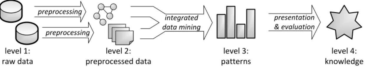
For an effective subspace clustering on imperfect data, we have to perform an integrated mining. By joining the preprocessing step with the actual mining task, we are able to account for the special characteristics of subspace clustering leading to a better handling of imperfect information. Figure 1.4 illustrates this integrated mining step: instead of mining the preprocessed data, the mining method directly analyzes the raw data and, e.g., instantiates missing values based on the currently detected subspace clusters.

Robust clustering models. Directly operating on imperfect data leads to novel requirements for subspace clustering models and definitions ranging from the ac-curate determination of similarity values between individual objects to the overall coherence of a cluster in an imperfect setting. The underlying challenge to be tackled by these models is their robustness against ’errors’ in the data. Even for a high-degree of imperfect information, reliably detecting high quality patterns should be possible.

In summary, the issues discussed so far focus on level 2 and 3 of the KDD process, and they assume a single representation of the objects by, e.g., a database of high-dimensional vectors. As the following section illustrates, the assumption of single data type has to be relaxed in many applications; we also have to adapt level 1 of the KDD process.

Challenges for Subspace Clustering on Heterogeneous Data

Traditional data mining algorithms process just a single type of data, e.g., objects embedded into a vector space. Today’s applications, however, can acquire multi-ple, diverse, and heterogeneous data sources. Besides characterizing single objects

(17)

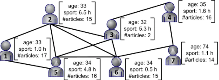
1.2. Subspace Clustering for Complex Data 11 age: 33 sport: 1.0 h #articles: 17 age: 33 sport: 6.5 h #articles: 15 age: 34 sport: 4.8 h #articles: 16 age: 32 sport: 5.3 h #articles: 2 age: 35 sport: 1.6 h #articles: 16 age: 34 sport: 0.5 h #articles: 15 age: 74 sport: 1.1 h #articles: 14 2 1 5 6 3 7 4

Figure 1.5: Exemplary social network represented by vector and graph data

by vector data, network information, for example, is a ubiquitous source to indi-cate the relations between different objects. Such type of heterogeneous data can be observed in various domains including social networks, where friendship rela-tionships are available along with the users’ individual interests (cf. Figure 1.5); systems biology, where interacting genes and their specific expression levels are recorded; and sensor networks, where connections between the sensors as well as individual measurements are given. While imperfect data, as introduced in the previous section, usually reduces the amount of information that can be utilized in the mining step, heterogeneous data increases this pool. Thus, to realize the full potential for knowledge extraction, mining techniques should consider all avail-able information sources. In this thesis we focus on heterogeneous data as given in the applications mentioned above because this type is one of the most prevalent ones. The general challenges for subspace clustering, however, apply for all types of heterogeneous data.

Integrated mining. A sequential process for heterogeneous data, which first mines each type independently and then compares the detected patterns, is prob-lematic since the results of each source might differ or even contradict. Thus, for an effective subspace clustering, again an integrated mining promises more meaningful and accurate results. By simultaneously mining different types of in-formation, as illustrated in the adapted KDD process of Figure 1.6, inaccurate information in one source can be mitigated by the other sources and an overall coherent result is possible.

By integrating heterogeneous information types into a single mining task, dif-ferent paradigms as graph mining and subspace clustering need to be joined. Since each paradigm has established its own objectives and even worse these objec-tives might contradict, e.g., large clusters vs. high dimensional clusters, a sound synthesis is highly challenging but actually crucial. We have to ensure that the

(18)

12 Overview of Thesis level 1: raw data level 2: preprocessed data level 3: patterns level 4: knowledge presentation & evaluation preprocessing preprocessing integrated data mining

Figure 1.6: Enhanced KDD process by simultaneously mining multiple information types for better handling of heterogeneous data

paradigms are treated on an equal footing and none of the data sources is favored over the other. Especially retaining the characteristic of subspace clustering — objects might be part of multiple patterns potentially inducing redundancy — is a challenge posed by mining heterogeneous data.

Efficient algorithms. Since the databases to be analyzed and the resulting patterns to be detected are inherently complex due to the heterogeneous types of information, the algorithms’ efficiency is an important aspect we have to cope with. Thus, developing novel pruning techniques or algorithms that efficiently provide an approximate mining result is a further requirement for today’s subspace clustering methods.

Summary

As shown in this section, for an effective subspace clustering on complex data various challenges have to be solved and novel techniques need to be introduced covering the first three levels of the KDD process. Only such novel models en-sure to detect meaningful patterns and, thus, potentially lead to new and useful knowledge.

1.3

Contributions and Structure of this Thesis

This thesis introduces models and algorithms for effective subspace clustering on complex data. To provide a holistic view on the KDD process, all aforementioned challenges are tackled in this work. The following section presents an overview of the major contributions and the general structure of this thesis while details are discussed in the subsequent chapters. The thesis is divided into four parts.

(19)

1.3. Contributions and Structure of this Thesis 13

Part 1: Subspace Mining on Vector Data

In the first part of this thesis we focus on subspace clustering methods for vector data. As our first contribution, we introduce our clustering model RESCU that avoids redundant information in the final clustering in Chapter 2. In contrast to existing approaches that simply exclude lower dimensional projections of clusters, our method introduces a global optimization approach taking all clusters simul-taneously into account. Our optimization ensures to select the most interesting clusters, where each cluster provides novel knowledge w.r.t. all other clusters in the final result. Unlike to projected clustering methods, which avoid redundancy by enforcing disjoint clusters, RESCU allows overlapping clusters in general by ex-tending the Set Cover optimization problem to the subspace clustering paradigm. Our model is highly flexible since it is independent of the underlying subspace cluster definition and the selected interestingness measures. We prove that the computation of our RESCU model is NP-hard, and we propose an algorithm deter-mining an approximate solution showing high clustering accuracy.

While RESCU successfully avoids redundant information, it is not able to detect multiple views in the data. Thus, as our second contribution, we introduce clus-tering models able to solve this challenge. In Chapter 3, we present our OSCLU method that judges the redundancy of clusters based on their similarity regarding objects and subspaces. The global optimization method of OSCLU actively in-cludes novel knowledge of (almost) orthogonal subspaces into the final clustering result. While our OSCLU model provides a general and flexible solution to detect subspace clusters hidden in multiple views, we prove its complexity to be NP-hard and propose an efficient algorithm to compute an approximate solution.

OSCLU is able to detect clusters hidden in multiple views. The views itself, however, are not explicitly mined, i.e., it remains unknown which clusters belong to the same view and which attributes are characteristic for this view. To overcome these limitations, we introduce our MVGen method in Chapter 4. Based on a generative model that considers the data as a result of a process generated by different views, we couple the detection of subspace clusters and their aggregating views. Using our novel representation, we perform Bayesian model selection to determine those dimensions which are relevant for the views and their subspace clusters, and we enable the detection overlapping clusters and overlapping views without inducing redundancy. Since exact inference in our model is intractable, we

(20)

14 Overview of Thesis

use the principle of iterated conditional modes to realize an efficient and effective clustering algorithm.

While the previous methods focus on clusters corresponding to dense areas in the data space, we propose in Chapter 5 a method which is able to detect more complex patterns. As our next contribution, we introduce the novel paradigm of subspace correlation clustering: we analyze subspace projectionsto find subsets of objects showing linear correlations among this subset of dimensions. While ex-isting correlation clustering methods are limited to almost disjoint clusters, our model allows each object to contribute to several correlations due to different subspace projections. In our paradigm, we permit multiple overlapping clusters but simultaneously avoid redundant clusters deducible from already known cor-relations originating from collinearity or induction. Furthermore, as known from traditional clustering, analyzing the full-space might be questionable due to the decreasing discrimination power of distances resulting from multiple overlapping patterns and irrelevant dimensions. Therefore, by analyzing individual subspace projections, our model opens the potential to detect correlations that clearly stand out in the data. We develop the algorithm SSCC, which exploits different pruning techniques to efficiently generate a subspace correlation clustering result.

Part 2: Subspace Mining on Imperfect data

In the second part of this thesis we focus on subspace clustering methods for im-perfect data. After introducing and classifying the various types of imim-perfect data in Chapter 6, we analyze two scenarios in detail: imperfect data due to missing values and imperfect data due to uncertainty about attribute values.

As our contribution in Chapter 7, we introduce a general fault tolerance defi-nition enhancing subspace clustering models to handle missing values. Our model handles missing values based on the currently considered subspace and set of ob-jects. It, thus, enables objects to be part of multiple subspace clusters. Our variable thresholds realize a flexible model that adapts to the individual cluster character-istics and ensures a robust parameterization. The high complexity of an integrated subspace clustering method handling missing values demands for effective prun-ing methods. Thus, we prove important monotonicity properties of our general model. In the experimental evaluation, our approach yields high quality results even in the presence of many missing values.

(21)

1.3. Contributions and Structure of this Thesis 15

In Chapter 8 we present an integrated mining method for subspace clustering on uncertain data. We present three variants that can be distinguished by the amount of information extracted from the probability density functions. Since for subspace clustering and especially in uncertain scenarios a strict assignment of objects to single clusters is not appropriate, we enrich our model with the con-cept of membership degree enabling a non-partitioning clustering result. To cope with the computational challenges of subspace clustering for uncertain data, we propose an efficient solution that uses Apriori-based pruning and heuristic sam-pling. Thorough experimental evaluation demonstrates that our integrated sub-space clustering method substantially outperforms competing techniques.

Part 3: Subspace Mining on Heterogeneous Data

In the third part of this thesis we develop subspace clustering methods for het-erogeneous data. We discuss the diversity of data types and mining challenges in Chapter 9, before we focus on the development of integrated clustering tech-niques simultaneously handling network data in combination with vector data in the subsequent chapters.

In Chapter 10 we introduce our GAMER method for finding homogeneous groups in such heterogeneous data by joining the paradigms of subspace clus-tering and dense subgraph mining. GAMER detects clusters that are optimized

according to their density, size, and number of relevant dimensions to fairly trade-off the different paradigms’ objectives and to obtain the most interesting clusters. GAMER confines the clustering by excluding redundant clusters but still allows

multiple views on the data. By incorporating both data sources we develop novel pruning strategies that lead to an efficient calculation of our clustering.

Extending the GAMER method, we develop our EDCAR model in Chapter 11.

EDCAR performs a global optimization to determine the overall clustering solu-tion and to avoid redundancy. As shown for tradisolu-tional vector data by our RESCU model, optimizing the clustering globally is beneficial but is usually more com-plex. We prove the complexity of our EDCAR model and identify the critical parts inhibiting an efficient execution. Based on this analysis, we develop an efficient and effective algorithm that approximates the optimal clustering solution. By in-terweaving the process of cluster generation and cluster selection, which both make use of the GRASP principle, we determine high quality clusters and ensure low runtimes.

(22)

16 Overview of Thesis

As our last contribution in this part, we introduce in Chapter 12 the DB-CSC model that adopts a density-based cluster definition to take the attribute similar-ity in subspaces and the graph denssimilar-ity into account. Even though the previously proposed approaches successfully overcome the problem of full-space clustering, their limited cluster definitions are restricted to clusters of certain shapes. Thus, introducing the novel notion of local densities, our DB-CSC model aims at detect-ing clusters of arbitrary shape and size. In contrast to density-based methods for vector data, calculating clusters in heterogeneous data is more challenging and we show how a fixed point iteration can be used to find the clusters. Using this princi-ple and further pruning techniques, our DB-CSC algorithm efficiently determines the combined clustering solution.

Part 4: Summary

In the last part, we conclude this thesis by summing up all contributions and by presenting open challenges for future work in the area of subspace clustering.

(23)

Part I

Subspace Mining

on Vector Data

(24)

(25)

Chapter 2

Relevant Subspace Clustering

In high-dimensional vector spaces, clusters rarely show up in the full dimensional space but are hidden in subspace projections of the data. Subspace clustering methods try to detect these patterns by analyzing arbitrary subspaces of the data for their clustering structure. In general, a subspace cluster C = (O, S)is defined by a set of objectsO ⊆DB that are similar in a subset of dimensionsS ⊆Dim.

As discussed in Chapter 1.2, naively performing subspace clustering yields to an overwhelming result of redundant clusters: often the objects grouped in cluster

C = (O, S)are also similar in the subspace projections S0 ⊆ S. Since the number of possible subspace projections is exponential in the number of dimensions, tra-ditional subspace clustering approaches generate a tremendously large result and they fail to detect only the relevant subspace clusters.

In this chapter, we propose our novel model for relevant subspace clustering (RESCU), detecting the most interesting non-redundant subspace clusters. In con-trast to existing methods, our global redundancy elimination checks the relevance of each cluster against all other possible subspace clusters. It aims at reporting as few clusters as possible to reduce redundancy, yet include as many interest-ing clusters as possible. The general idea is to cover almost all objects (except of noise) by interesting clusters. Thus, we allow overlapping subspace clusters in general but require each cluster to contribute at least some novel knowledge by grouping additional objects. Overall, the result is optimized based on the user’s specified interest and our global redundancy notion.

(26)

20 Relevant Subspace Clustering

2.1

Motivation and Comparison with Related Work

In the last decades several methods for clustering in subspace projections were proposed. In general, we can distinguish two different paradigms: subspace clus-tering and projected clusclus-tering.

Subspace clustering. Subspace clustering detects clusters in arbitrary projec-tions by automatically determining a set of relevant dimensions for each cluster [PHL04, KKZ09]. Thus, one is able to detect objects as part of various clusters in different subspaces. In bioinformatics, for example, genome data analysis clusters genes (objects) that show similar expression levels in a subset of experimental medical treatments (attributes). Such similarities might indicate functional re-lationships. Each gene might appear in multiple roles (subspace clusters). As a consequence, subspace clusters might overlap in the sense that they share ob-jects. Starting with the first subspace clustering approach CLIQUE [AGGR98], recent research has seen a number of approaches using different definitions of what constitutes a subspace cluster [AGGR98, KKK04, SZ04, KKRW05, NGC01]. As summarized in a recent evaluation study [MGAS09], their common problem is that the output generated is typically huge.

Subspace clustering allows clusters to overlap, but has to cope with the de-tection of exponentially many subspace clusters in arbitrary projections. Many of these clusters do not provide any further information, as more or less the same object groups are detected in multiple projections of the data. Such redundant subspace clusters should be removed and only the most interesting ones, which provide novel knowledge about the data should be reported.

Some approaches towards modeling and removing redundant subspace clus-ters have been proposed. They define non-redundant and possibly overlapping subspace clusters, but only with a local scope. In [AKMS07, AKMS08a, AKMS08b], a subspace cluster is redundant if it shares a certain fraction of objects with an-other one. Retaining only maximal subspace clusters, i.e. the highest dimensional one of two, results in a clear increase in clustering quality. This is due to the fact that maximal clusters tend to contain less noise and thus represent the inherent data structure more faithfully. This definition of redundancy, however, is limited in two respects. First, redundancy is based only on a pairwise comparison of clus-ters. And second, the redundancy check incorporates only the fraction of jointly detected objects [AKMS07, AKMS08a, AKMS08b]. We call this a local redundancy definition, as only local properties like object count and comparison of two

(27)

sub-2.1. Motivation and Comparison with Related Work 21

space clusters is used. Consequently, a redundant subspace cluster that is covered by a combination of high dimensional subspace clusters is still reported as non-redundant. In contrast, our model aims at a global redundancy check including a more flexible interestingness definition comparing each cluster with the overall set of detected subspace clusters.

Another subspace clustering approach aims at extracting non-redundant axis-parallel subspace regions [MS08]. It defines non-redundant results as the min-imal subset of subspace clusters to approximately compute the support of any other subspace cluster (assuming uniform distribution otherwise). This statistical approach, however, is based on the assumption of uniform distribution inside a cluster. Moreover, the redundancy model is limited to the fixed cluster definition.

Projected clustering. The paradigm of projected clustering was introduced by the PROCLUS method [AWY+_{99]. Inspired by traditional partitioning clustering}

methods like k-Means, projected clustering [AWY+_{99, MSE06, YCN05, BKKK04,}

YM03, PJAM02] partitions the data into disjoint clusters but simultaneously de-termines the most relevant dimensions for each group. Thus, projected clustering assigns each object to at most a single cluster. A partitioning of the data into projected clusters can be regarded as extreme redundancy elimination. Projected clustering results in a manageable number of clusters, but is not able to detect overlapping clusters. By limiting the clustering model to handle only disjoint clus-ters several meaningful clusclus-ters are only detected in parts or they are completely lost. In many application scenarios this is a general drawback, which is not ac-ceptable for clustering in subspace projections.

As we show in our evaluations all of the existing approaches fail to detect all but only the hidden subspace clusters in a high dimensional database.

Contributions of the RESCU model. Our goal is to derive a novel model for non-redundant subspace clusters that takes a global look at overlapping clusters. The aim is to find all but only relevant clusters by optimizing the overall clustering result. The main contributions of our work are:

• Detection of all interesting clusters, but without the overwhelming result size of subspace clustering.

• Detection of only non-redundant clusters, but without the strict partitioning of projected clustering.

(28)

sub-22 Relevant Subspace Clustering

space clustering. We combine an interestingness function for subspace clusters with a coverage criterion for an overall redundancy removal. By including the most interesting clusters and excluding redundant clusters, our result set contains all but only relevant subspace clusters. Any object can be part of multiple clusters, allowing overlapping subspace clusters. Furthermore, our relevance model is nei-ther restricted to one cluster definition nor based on a fixed interestingness rating. These two aspects are typically application dependent and can be adapted by the instantiation of our model. Considering computation complexity, we prove that our relevant subspace clustering is NP-hard. Thus, for an efficient computation of our relevance model we propose an heuristic algorithm generating possible cluster candidates in best-first order according to their relevance.

2.2

Relevant Subspace Clustering

In this section, we introduce our relevant subspace clustering definition. Our model is independent of a certain subspace cluster definition, as e.g. density-based clusters [KKK04, AKMS07], but we simply assume that the set All = {C1. . . Cn}

of all subspace clusters that fulfill the selected definition is given. Note: As pre-computation of All is usually too expensive we propose an heuristic algorithm using an on-demand cluster generation derived from our relevance model in Sec-tion 2.3. Most of the clusters in All do not provide any knowledge for the user, thus, our relevance model defines which of these clusters to output (cf. Fig. 2.1). In our model we utilize a global view for redundancy elimination, which considers the whole setAll at the same time. Overall, we aim at reducing the output to only therelevantsubspace clusteringRes⊆All. The remaining clusters overwhelm the user, thus hinder the analysis and are removed.

Two aspects are important for relevance. One is theinterestingnessof a cluster itself. The interestingness evaluates a cluster locally via its properties like dimen-sionality or size. For example, clusters in located in one-dimensional subspaces might not be interesting. Interestingness is often user or application dependent and therefore it should be adaptable. A detailed discussion of our flexible inter-estingness model is given in Section 2.2.1.

Another aspect is theredundancyof clusters. Redundancy means that this clus-ter does not contribute to new knowledge with respect to other clusclus-ters (for exam-ple if another cluster with similar properties exists). Consequently, a redundant

(29)

2.2. Relevant Subspace Clustering 23 all possible clusters All relevance model interestingness

of clusters redundancyof clusters

relevant clustering

Res All

Figure 2.1: Components of a relevance model

cluster should not be reported. The redundancy is discussed in Section 2.2.2. Please note that the two aspectsredundancyandinterestingnessare not entirely independent in our model but they are considered simultaneously. We include the most interesting clusters but exclude redundant clusters of low interest. Thus, the user specified interest is also used in the redundancy elimination. Given the choice between two clusters with similar properties, the less interesting one should be marked as redundant. Overall, our optimization excludes both clusters with low interest and clusters that cover too few new objects (not yet covered by other clus-ters). This interleaved handling of interest and coverage of new objects is the key property of our optimization: a relevant cluster is interesting but not redundant.

Our overall relevance model is described in Section 2.2.3. We prove important complexity results in Section 2.2.4, discuss the parameters of our approach in Section 2.2.5 and conclude in Section 2.2.6 with an instantiation of our model.

2.2.1

Interestingness of a cluster

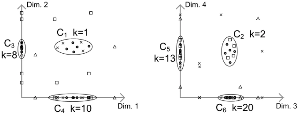
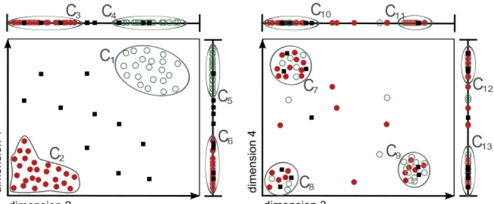
In this section, we describe the flexible interestingness model of RESCU to quantify the interestingness of a single cluster. Figure 2.2 gives an example of clusters in dimensions 1 and 2 (left), and 3 and 4 (right), respectively. Objects in both illustrations are represented using the same symbol. For example, assume that we deem clusters with more dimensions more interesting. The two-dimensional clustersC1andC2 are then favored over the one-dimensional clustersC3−C6. The

number of objects, the diameter or the density of a cluster are other typical choices of interestingness. Besides these user driven specifications, further measures using statistical properties of the data might also be applicable and are widely used in other research areas such as frequent itemset mining [GH06, ST96]. By analyzing the data’s distribution, such measures provide more objective criteria to evaluate the interestingness of a pattern and can be integrated in our model. However, as we focus more on the general perspective and the interleaved usage of interest in

(30)

24 Relevant Subspace Clustering

our relevance model, we select a simple user-dependent interestingness measure based on the size and/or dimensionality of a cluster (cf. Section 2.2.6).

For the general perspective, let us discuss how interestingness is currently used (or not used) in subspace and projected clustering methods. Interestingness is not handled explicitly in existing projected clustering approaches. Since overlapping clusters are not permitted, the most interesting clusters, e.g. C1 and C2 in Figure

2.2, may not be found. They both contain some objects that occur in the other clus-ter as well, and are therefore mutually exclusive. As a consequence, potentially interesting clusters are missed by the occurrence of otherinteresting clusters. An-other problem is the handling of outliers only in a post-processing step. Since the interestingness of clusters, e.g. their compactness, is calculated before removal of outliers, misleading values can occur.

Subspace clustering algorithms realize only a very limited interestingness cal-culation. Each set of points and dimensions that fulfills the cluster definition (e.g. exceeding a density threshold) is equally interesting. Thus, there is no specifica-tion of different degrees of interest in subspace clustering. It is a binary decision “cluster” or “no cluster”. The user is not able to control what kind of clusters he is more interested in. After detecting all subspace clusters, no additional selection of the most interesting clusters out of the huge result set is performed.

Finally, the calculation of the interestingness in both models is usually fixed (or at least limited to the parameters introduced by the methods’ developers) and cannot be modified by the user. A general and flexible interest specification pro-viding the ability to instantiate the model by the application dependent needs is not provided. C1 k=1 C4 k=10 C3 k=8 C6 k=20 C5 k=13 C2 k=2 Dim. 1 Dim. 3 Dim. 2 Dim. 4

(31)

2.2. Relevant Subspace Clustering 25

Our model overcomes these problems. We assign an (un-)interestingness value to each cluster. It is a local rating, i.e. other clusters do not influence this measure. Furthermore, our cluster definition (cf. Sec. 2.2.6) accounts for outliers. Thus, misleading values do not occur.

As a general and flexible framework, we model the (un-)interestingness via a cost functionk. Intuitively, uninteresting clusters should get a high cost value since the benefit of analyzing these clusters during the knowledge discovery process is low but they only lead to high cost since, e.g., human resources or storage capac-ities are wasted for the analysis. Accordingly, small cost values denote interesting clusters. For any clusterC, given by the set of its objectsO and the corresponding dimensionsS, we define the cost function as follows:

Definition 2.1 Cost function for subspace clusters

LetP(DB)be the power set of all database objects and P(Dim)the power set of the dimensions. A cost function

k:P(DB)× P(Dim)→_R

assigns costk(O, S)to the subspace clusterC = (O, S).

Please note that the domain of the cost function is not modeled byP(DB×Dim). In this case, a single clusterC could contain objects that belong to different sub-spaces. For traditional subspace clustering, however, each objecto ∈O of a given subspace clusterC = (O, S)is associated with the same subspaceS.

Exemplary cost values are depicted in Figure 2.2, where the one-dimensional clusterC4 gets a cost value ofk = 10while the more interesting two-dimensional

cluster C1 gets a lower cost value of k = 1. By defining a cost function, we can

account for several aspects of a subspace cluster, like the dimensionality or the density. Changes to the cost function yield an easy adaptation of the model. This flexibility is not achieved by other approaches. By first calculating the interesting values individually and allowing overlap we find higher quality clusterings. In Figure 2.2 we may select bothC1 and C2.

For computational reasons, we assume cost functions which assign a strictly positive value to all subspace clusters, i.e. given a setM ={(O1, S1), . . . ,(On, Sn)}

of clusters, the function fulfills k(Oi, Si) > 0 for all (Oi, Si) ∈ M. To mine the

(32)

26 Relevant Subspace Clustering

the number of objects covered by a clustering, we additionally take coverage into account. We formalize coverage as follows:

Definition 2.2 Coverage of a clustering

Given a clustering M = {(O1, S1), . . . ,(On, Sn)}, the coverage of M is defined as

follows: Cov(M) =Sn i=1Oi

The coverage of a clusteringM is the union of the objects in all selected clusters. We now define the overall relative cost of a clustering as the sum of the individual cost values normalized by the number of covered objects.

Definition 2.3 Overall relative cost of a clustering

Let M = {(O1, S1), . . . ,(On, Sn)} be a clustering andk a cost function for subspace

clusters. We define the overall relative cost ofM as:

RK(M) = K(M)

|Cov(M)| withK(M) =

X

(Oi,Si)∈M

k(Oi, Si)

The smaller the overall relative costRK(M), the more interesting is the clustering

M per covered object. Thus, we trade off the total cost of a clustering against its coverage. We achieve a high coverage and at the same time small total cost.

2.2.2

Redundancy of a cluster

The second aspect of relevance is non-redundancy. A large clusterC and all of its lower dimensional projections could be assigned low cost values if interestingness is based on size. Selecting all projections along with C based on interestingness alone leads to a poor overall result. One gets very many redundant clusters, while

C would be sufficient.

Existing projected and subspace clustering algorithms do not address redun-dancy handling adequately. Projected clustering simply forces results to be non-redundant by assigning each object to a single cluster at the cost of missing over-lapping clusters. Subspace clustering algorithms, in contrast, either use no or a mere local approach to check the redundancy. Such an approach compares only two clusters [AKMS07, AKMS08a, AKMS08b]. If the clusters cover nearly the same objects, one of them is redundant. The problem of this local approach is illustrated

(33)

2.2. Relevant Subspace Clustering 27

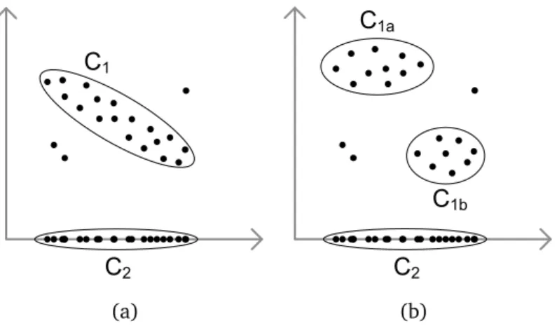
in Figure 2.3. Obviously, in both subfigures, the clusterC2 is redundant because it

is induced by the other clustersC1, resp. C1a,C1b. A local approach could identify

the redundancy in the left figure. ClusterC2 is redundant, as it coversC1 and only

a few additional objects. In the right figure, the fraction of points shared by C1a

andC2 as well as by C1b andC2 is small, and the clusterC2 is misleadingly

classi-fied as non-redundant. This mistake is the result of the local view on redundancy, i.e. for each check only a pairwise comparison of clusters is performed.

C1 C2 (a) C1a C1b C2 (b)

Figure 2.3: Local and global redundant clusters

We use a global view for the redundancy checks, i.e. we use all clusters at the same time to judge the redundancy of another cluster. This approach results in more accurate decisions. While the interestingness is a local measure based on the cluster itself, the redundancy takes other clusters into account.

As one can see from the above example, the redundancy of a cluster is linked to the coverage of objects. If a set of clusters shares many objects with a clusterC,C

is a redundant cluster. In other words: A cluster is redundant if it does not cover many new objects. The cluster C2 in Figure 2.3(b) is redundant, because with

respect to the two other clusters only a few new objects are covered. The same holds for the clusterC2 in Figure 2.3(a). The fact that we consider all clusters for

the redundancy checks yields a global redundancy model. Thereby we identify in both subfigures the clusterC2 as redundant.

Basic Set-Cover approach If we select theminimalnumber of clusters such that all objects are covered, we can realize a global redundancy model. The output of clusters that only contain already covered objects is prevented. This check is

(34)

28 Relevant Subspace Clustering

performed with respect to all other clusters in the result set. At the same time, we identify multiple overlapping clusters in the data because all objects have to be covered.

This novel way of subspace clustering can be considered as an instance of the Set-Cover problem [GJ79]. Given several finite sets, Set-Cover seeks for the mini-mal number of sets that cover the whole population. In the clustering context, we want to find the minimal number of clusters such that all objects are covered.

However the direct application of Set-Cover to our task is not possible.

Problem 1: Simply choosing the minimal number of clusters means that usu-ally low dimensional clusters, which tend to contain more objects, are preferred over high dimensional clusters. This preference usually conflicts with the user’s notion of interestingness. Instead of choosing the minimal number of clusters, we determine the clustering with minimal relative cost (cf. Def. 2.3). This setup takes the desired interestingness notion into account. In Figure 2.3(b), for exam-ple, we would choose the two two-dimensional clusters instead of the one one-dimensional cluster. We thus use an extension of the Set-Cover problem to the Weighted-Set-Cover problem [Chv79].

Problem 2: Covering all objects by clusters is not always a meaningful solution, as some databases contain outliers that do not fit to any cluster. The Set-Cover problem enforces a complete cover of all objects and potentially finds no solution in this case. Or all objects are covered by uninteresting clusters only. For example, if the outliers are only contained in the one-dimensional clusters, the Set-Cover problem enforces choosing these uninteresting ones. An example is depicted in Figure 2.3(b), as one has to select C2 to get a complete coverage. We therefore

propose a generalization of the Set-Cover problem to cope with outliers.

Gain-based redundancy We solve these problems by a gain-based extension of the Set-Cover problem. The basic idea is to measure the gain of a new cluster if we add it to a known clustering. In other words, we have to answer the question: Is it worthwhile to take the “more complex” clustering?

Let us consider Figure 2.4 and assume the clusters C1 and C2 to be selected.

Intuitively, the clusterC3is redundant with respect to the selected ones, so its gain

should be small. Two important aspects contribute to this fact. First, the cluster

C3 covers only a few new objects, i.e. many objects are already contained in other

(35)

2.2. Relevant Subspace Clustering 29 C1 k=1 C2 k=2 C4 k=8 C3 k=10 C5 k=9 clus gain(C3,{C1, C2}) = ₁₀3 = 0.3 clus gain(C4,{C1, C2}) = 1₈ = 0.13 clus gain(C2,{C1}) = 8₂ = 4 clus gain(C1,{C2}) = 10₁ = 10 K({C1,C2}) |Cov({C1,C2})| = 3 18 = 0.17 K({C4,C5}) |Cov({C4,C5})| = 17 21 = 0.81

Figure 2.4: Relevant clustering

via the residual set O\Cov({C1, C2}). And second, the cost of the cluster is very

high, i.e. the cluster is not interesting. High costk(O, S)should correspond to a low gain. Overall we take the ratio of these two measures. Cluster gain thus is the additional coverage in relation to its cost.

Definition 2.4 Cluster gain

Given a cluster C = (O, S), a clusteringM and a cost functionk for M ∪ {C}. The cluster gain ofC with respect toM is:

clus gain(C, M) = |O\Cov(M)| k(O, S)

We identify a cluster as redundant (with respect to a given clustering) if its cluster gain is smaller than a user-defined threshold ∆. In Figure 2.4 the cluster gain of C3 (with respect to {C1, C2}) is only 0.3 as C3 covers 3 new objects and k(C3) = 10. Instead,C2 has a higher cluster gain of4(with respect to{C1}).

Consistent with this idea, a clusteringM is redundancy-free ifallclusters fromM

exceed the selected minimal cluster gain∆. The gain is measured with respect to the remaining clusters fromM so that each cluster adds sufficient information to the overall clustering.

Definition 2.5 Redundancy-free clustering

Given a clusteringM ⊆All and a minimal cluster gain ∆∈ _R≥0_{. The clustering}_M

is redundancy-free, iff

(36)

30 Relevant Subspace Clustering

In this way we achieve a global view for the redundancy checks. Each subspace cluster C has to compete with all remaining clusters M\{C} in the result set at the same time.

As one can see, the clustering {C1, C2}in Figure 2.4 is redundancy-free while the

clusterings {C1, C2, C3} or{C1, C2, C4}contain redundant information (assuming

∆ = 0.5). Definition 2.5 gives us the basis to avoid redundancy in our clus-tering. However, if we remove clusters from a redundancy-free clustering, this property still holds for the smaller clustering. The removal of information, i.e. clusters, cannot generate redundancy. This means that also the empty clustering is redundancy-free. That is obviously not desired by the user. To obtain a rele-vant clustering, it should be redundancy-free but at the same time cover as many objects as possible.

2.2.3

Overall relevance of a clustering

To enforce the selection of clusters we introduce the property of concept-covering. A clustering M does not satisfy this property as long as clusters exist that have a high gain and are not in M. M is not the result because further interesting concepts, represented by sets of clusters, can be covered. A clustering is concept-covering, and hence the coverage is sufficient, if all remaining clusters have a small cluster gain. We formalize this by:

Definition 2.6 Concept-covering clustering

Given a clustering M ⊆ All and a minimal cluster gain∆ ∈_R≥0_{. The clustering}_M

is concept-covering, iff

∀C∈All\M :clus gain(C, M)≤∆

Intuitively, a clustering is concept-covering if adding any new cluster always results in redundancy. A concept-covering clustering in Figure 2.4 is {C1, C2}.

Clustering {C1} is not concept-covering because we could add C2 without

intro-ducing redundancy.

The property of concept-covering clusterings is a relaxation of complete cover-age. It solves the problem of enforcing a complete coverage as in the Set-Cover problem (cf. Problem 2).

(37)

2.2. Relevant Subspace Clustering 31

RESCU: Relevant subspace clustering Our RESCU model demands a relevant clustering to be redundancy-free and concept-covering. However, as the exam-ple in Figure 2.4 illustrates, several clusterings could fulfill both properties, e.g.

{C1, C2} or {C4, C5}. To select the most interesting clustering, we additionally

compare their relative cost (cf. Def. 2.3). Our relative cost function (cost per cov-ered object) ensures finding an optimal clustering with both interesting clusters and high coverage. The relative cost for the clustering {C1, C2} in Figure 2.4 is

just0.17, but0.81for{C4, C5}. This is formalized by:

Definition 2.7 Relevant subspace clustering (RESCU)

Given a clusteringRes ⊆ All and a minimal cluster gain ∆∈ _R≥0_. _Res _{is relevant,}

if and only if

• Resis redundancy-free (Def. 2.5) and concept-covering (Def. 2.6) AND

• Reshas minimal relative cost, i.e.RK(Res)≤RK(N)

for all redundancy-free and concept-covering clusteringsN ⊆All

The relevant clustering in our previous example is thus {C1, C2}. Also for the

example in Figure 2.2 the relevant clustering is {C1, C2} even though the two

clusters share some objects. This illustrates that handling of overlapping clusters is possible in our model.

The flexibility of our model additionally provides the possibility of classifying other clusterings as relevant by changing the interestingness criterion. If we adapt the cost function so thatC1andC2in Fig. 2.4 get higher cost values, the clustering

{C4, C5} could become relevant. Thus our model enables the user to control the

output as desired.

2.2.4

Complexity analysis

In the following we show that calculating a RESCU clustering is an NP-hard prob-lem. We prove this by giving a polynomial reduction of the Weighted-Set-Cover problem, which is a NP-complete problem, to our RESCU model, i.e. we prove Weighted-Set-Cover ≤p RESCU. The Weighted-Set-Cover problem seeks those

non-empty sets that together have minimal weights and fully cover all objects. For this reduction we need to map the input of the Weighted-Set-Cover problem to an

(38)

32 Relevant Subspace Clustering

input of RESCU and show that the resulting relevant subspace clustering is a valid solution for the Weighted-Set-Cover problem.

Theorem 2.1 Computing RESCU (Def. 2.7) is NP-hard. Proof 2.1

We show that Weighted-Set-Cover ≤p RESCU.

Input mapping: We map the input of the Weighted-Set-Cover (objects, sets, weight function) to an input for RESCU (database DB, possible clusters All, cost function

k). We map the assumption of the Set-Cover (complete coverage exists) to (∆=0) in RESCU. We now have to show that relevant subspace clustering (cf. Def. 2.7) corre-sponds to a solution of the Weighted-Set-Cover problem.

RESCU generates a valid solution for Set-Cover:

(1) Every chosen set contributes at least one object to the overall coverage: A relevant clusteringResis non-redundant (Def. 2.5):

⇔ ∀C ∈Res:clus gain(C, Res\{C}) = |O\Cov_k₍(_O,SRes₎\{C})| >0

Thus, all sets contribute at least one object

∀C∈Res:O =Cov({C})6⊆Cov(Res\{C}).

(2) For a Weighted-Set-Cover all objects have to be covered by at least one set: A relevant clusteringResfulfills the concept-covering property (Def. 2.6):

⇔ ∀C ∈All\Res:clus gain(C, Res) = |O\Cov_k₍_O,S(Res₎ )| ≤0

⇔6 ∃C ∈All\Res: |O\Cov(Res)|>0

Thus, all objects are covered: Cov(Res) =DB. (3) The sum of weights is minimal for the chosen sets:

A relevant clusteringReshas minimal relative costs (Def. 2.7): For all non-redundant and concept-covering clusterings

N ⊆All: RK(Res)≤RK(N)⇔ _|_CovK(Res₍_Res)₎_| ≤ _|_CovK(N₍_N)₎_|

FromCov(Res) =Cov(N) = DB we have: K(Res)is minimal.

(1)∧(2)∧(3)⇒Resis a valid Set-Cover solution. ⇒RESCU is NP-hard. 2 As we have proven, RESCU is a generalization of the Set-Cover problem and thus NP-hard. Furthermore, it has two advantages for detection of relevant clus-terings. First, we can handle outliers so that we can find a solution even if a complete coverage is not possible. And second, RESCU incorporates clustering properties and thus mines the most relevant clusters instead of simply covering the data.

(39)

2.2. Relevant Subspace Clustering 33

2.2.5

Discussion of Parameters

Our RESCU model requires just a single parameter: ∆. The parameter specifies the minimal gain each cluster of the result has to exceed. The parameter can be selected in the range[0, maxg)wheremaxg = max(Oi,Si)∈All

|Oi|

k(Oi,Si) is the maximal

gain a single cluster can achieve. For∆≥maxg, the result will be empty. By

low-ering the parameter, redundancy is evaluated less strict, i.e. clusters are allowed to overlap to a higher degree. For ∆ → 0 arbitrary overlap between clusters is possible as far as a cluster is not completely covered by other clusters.

Furthermore, the parameter ∆ intuitively controls the maximal relative cost the user is willing to accept for the final result. It holds that the relative cost of an optimal RESCU clustering Res ⊆ All is upper bounded by |DB_∆|. Since

|Cov(Res)| ≥P

Ci∈Res|Oi\Cov(Res\Ci)|and each cluster covers at least one

addi-tional object compared to the remaining clusters, we get RK(Res) = _|_CovK(Res₍_Res)₎_| ≤

P

Ci∈Resk(Oi,Si)

P

Ci∈Res|Oi\Cov(Res\Ci)| (∗) ≤ P Ci∈Res k(Oi,Si) |Oi\Cov(Res\Ci)| < P Ci∈Res 1 ∆ = |Res| ∆ ≤ |DB| ∆ . The

inequality (∗) is true as shown by the following theorem.

Theorem 2.2 (Sum inequality) Letn1, . . . ,nmandd1, . . . ,dmbe two sequences with

ni ∈R+0,di ∈R+ for alli∈ {1, . . . , m}. It holds:

Pm i=1 ni di ≥ Pm i=1ni Pm i=1di

Proof 2.2 LetL= maxi∈{1...,m}{n_di

i}. We get Pm i=1 ni di (1) ≥ L=L· Pm i=1di Pm i=1di = Pm i=1L·di Pm i=1di (2) ≥ Pm i=1ni Pm

i=1di Inequality (1) holds, since each term

ni

di is non-negative. Inequality (2) holds,

since for alliwe haveL≥ ni

di ⇔L·di ≥ni anddi is positive. 2

Thus, overall our model ensures the bound RK(Res) < |DB_∆| for an optimal RESCU clusteringRes⊆ All. This result can, for example, be used to find appro-priate parameter settings for ∆. For example, if the user selects a cost function that rates the dimensionality of clusters and if the user wants to ensure that the average dimensionality of the clusters in the final result exceeds a certain value, we can derive a value for∆guaranteeing this property.

2.2.6

Instantiation of the model

By the flexibility of our model we can handle any definition of subspace clusters (as the input of the model) and cost functions (to rate the clusters). For a practi-cal evaluation we instantiate these two aspects: for the cluster definition we use

(40)

34 Relevant Subspace Clustering

the frequently used paradigm of density-based clusters, while the cost function is based on the dimensionality of the clusters.

Definition of subspace clusters. We use density-based clustering because it de-tects clusters of arbitrary shape and size even in noisy data [EKSX96]. The idea is to define clusters as dense areas separated by sparsely populated areas. In this way outliers are not part of the clusters within the same subspace, and mislead-ing ratmislead-ings are prevented. An object is considered dense if its neighborhood, i.e. an ε-distance region around it, is sufficiently populated. We follow the definition from [KKK04] with the modification that we adjust the ε-range according to the subspace dimensionality. Thereby we account for increasing distances between the objects in higher dimensional spaces. Thus, a subspace cluster is defined by Definition 2.8 Given a set of dimensions Dim = {1, . . . , D}, a database of objects

DB ⊂_RD_{, and an adaptive neighborhood range function}_ε₍_d_{) :}

N→R+, a subspace

cluster C= (O, S)withO ⊆DB andS ⊆Dimfulfills the following properties: (1) high density: ∀o∈O :|{p∈DB |distS(o, p)≤ε(|S|)}| ≥τ

(2) density connected: ∀o, p ∈ O : ∃o1, . . . , ok ∈ O : o1 = o ∧ ok = p∧ ∀i = 1, . . . , k−1 :distS(oi, oi+1)≤ε(|S|)

(3) maximality: ¬∃O0 ⊃O fulfilling (1) and (2) where distS(o, p) =

pP

i∈S|o[i]−p[i]|2 is the Euclidean distance restricted to the

subspaceS.

While traditional density-based clustering methods and many subspace clus-tering approaches use a constant neighborhood range, we use a monotonically increasing function ε(d). Since the distance between objects increases with in-creasing subspace cardinality, using a constant density criterion is problematic: By using a small ε (or large τ) we cannot expected any high dimensional clusters; most objects have a distance larger thanε. By using a largeε(small τ), however, the low dimensional clusters are no longer meaningful since they group nearly all objects in a single cluster; most objects have a distance smaller than ε. A den-sity criterion that is identical for each subspace is not an appropriate choice for subspace clustering. We have to use an adaptive density measure.

In general, the density calculation can be adapted to the subspace cardinality by modifying eitherε, i.e. the neighborhood range, orτ, i.e. the minimal number

(41)

2.2. Relevant Subspace Clustering 35

of objects in the neighborhood. While an adaption of ε directly antagonizes the increasing distances, τ acts only indirectly (increasing distances → fewer objects inε-neighborhood→smallerτ).

The indirect adaptation based on τ, as for example performed by [AKMS07, SZ04], is problematic since the value ofτ quickly converges to 0, i.e. even objects with just a single neighbor are reg