Global Comparison of CFD and Wind-Tunnel-Derived Force and Moment Databases for the Space Launch System

(1)

American Institute of Aeronautics and Astronautics 1

Global Comparison of CFD and Wind-Tunnel-Derived Force

and Moment Databases for the Space Launch System

Michael J. Hemsch*

ViGYAN, Inc., Hampton, VA, 23666

Recently a very large (739 runs) collection of high-fidelity RANS CFD solutions was obtained for Space Launch System ascent aerodynamics for the vehicle to be used for the first exploratory (unmanned) mission (EM-1). The extensive computations, at full-scale conditions, were originally developed to obtain detailed line and protuberance loads and surface pressures for venting analyses. The line loads were eventually integrated for comparison of the resulting forces and moments to the database that was derived from wind-tunnel tests conducted at sub-scale conditions. The comparisons presented herein cover the ranges 0.5≤M_∞≤5, ₋6°≤α ≤6°, and −6°≤β ≤6°. For detailed comparisons, slender-body-theory-based component build-up aero models from missile aerodynamics are used. The differences in the model fit coefficients are shown to be relatively small except for the low supersonic Mach number range, 1.1≤M_∞≤2.0. The analysis is intended to support process improvement and development of uncertainty models.

Nomenclature

BMC balance moment center (also reference moment center and approximate location of the vehicle _{center of gravity)}

DB database

Cm pitching-moment coefficient about the BMC

Cm0 zero intercept of the linear fit to the Cm versus CN data

CN normal-force coefficient

CN_α slope of the linear fit to the CN versus α data

CN0 zero intercept of the linear fit to the CN versus αdata.

Cn yawing-moment coefficient about the BMC

Cn0 zero intercept of the linear fit to the Cn versus CY data

CP center of pressure

CY side-force coefficient

C_Y_β slope of the linear fit to the CY versus βdata

CY0 zero intercept of the linear fit to the CY versus βdata.

M_∞ Mach number

RANS Reynolds-Averaged Navier-Stokes

SBT slender-body theory

SLS Space Launch System

WT wind tunnel

WTDB wind-tunnel-derived database ˆ

xCN fit to the CNaxial location of the CP, normalized by the reference length (core diameter) ˆ

xC_Y fit to the CYaxial location of the CP, normalized by the reference length (core diameter)

α angle of attack in body coordinates β sideslip angle in body coordinates

*_{Consultant, Associate Fellow.}

(2)

Introduction

The NASA Space Launch System (SLS) is intended to be the United States very-heavy launch vehicle for the foreseeable future (see Fig. 1). The first vehicle in the series, the Block 1 SLS-10003, will be used for the launch of the unmanned Orion space capsule around the moon and back (EM-1). For the purposes of various customers, the SLS Aerodynamics Task Team conducted wind tunnel tests in order to derive a comprehensive force and moment (F&M) database for ascent aerodynamics. Those subscale tests and subsequent development of the WT database are discussed in Pinier et al1_{. To complement the force and moment WTDB, a comprehensive CFD campaign was} conducted to provide line and protuberance loads and venting data. The CFD campaign obtained very high fidelity Reynolds-Averaged-Navier-Stokes solutions at 739 ascent conditions (full-scale) in the ranges 0.5≤M_∞≤5,

−6°≤α ≤6°, and −6°≤β ≤6°. The overset grid system consisted of 375 million grid points. The details of the CFD campaign are presented in Rogers et al2_.

It is unusual in the uncertainty community to have such a large set of CFD solutions for comparison with

experimental (wind tunnel) data. Of course, the CFD solutions were obtained at full-scale flight conditions while the wind tunnel database was derived from subscale tests, albeit with the model gritted for boundary layer transition1_. Nevertheless, comparing the CFD with the WTDB for quality control checks and for potential uncertainty modeling seems reasonable and useful. The following four sections present the CFD-to-WTDB comparisons for the normal-force coefficient,C_N, the side-force coefficient,C_Y, the pitching-moment coefficient,C_m, and the yawing-moment coefficient,C_n, respectively. The axial-force and rolling-moment coefficients are not considered in the paper.

The CFD and WTDB results can, of course, be compared by simple subtraction and those results are given below. However, it is possible to do more detailed comparisons using modeling appropriate for the given conditions. For that purpose, slender-body-theory-based component build-up aero models3-5_{from missile aerodynamics are} selected. For simplicity, the models will be designated by the acronym, SBT, for the rest of the paper. It should be noted from the references that SBT can be applied to any airframe provided that the airflow is sufficiently "slender".

Normal-Force Coefficient

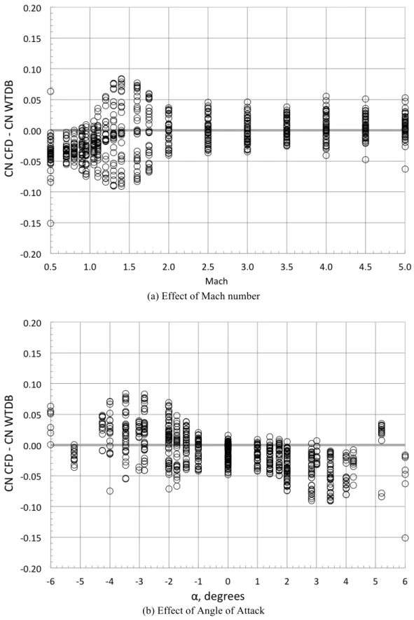
Simply subtracting the WTDB C_N results from the CFD C_N results for all of the conditions in the CFD 739-run matrix gives the plots shown in Fig. 2. Fig. 2(a) shows the differences between the two types of angle-of-attack polars at the breakpoint conditions as a function ofM_∞, revealing that the lower supersonic conditions have almost double the scatter of the rest of the differences. Fig. 2(b) shows the effect of angle of attack on the scatter of the differences. The Mach number breakpoints of the CFD database are visible as the abscissa locations of the columns of symbols in Fig. 2(a). Note that it is difficult to discern much of a pattern in Fig. 2. To be able to discern any patterns associated with the three independent variables of M_∞, α, and β , it is necessary to model the dependent variables as functions of the independent variables. The rest of the paper will describe the modeling choices and the results.

It has long been known that first-order SBT3, 4, 6, 7_predicts_C

N to be a linear function of α only, independent ofβ andM_∞. Wind tunnel testing of slender airframes over many years has shown, however, that C_Nis a weak function of M_∞. Given that information, the following linear equation is used to model the C_Ndependence with eachM_∞ treated separately. Least squares is used to choose the coefficients:

C_N=C_N

0+CNαα

(1)

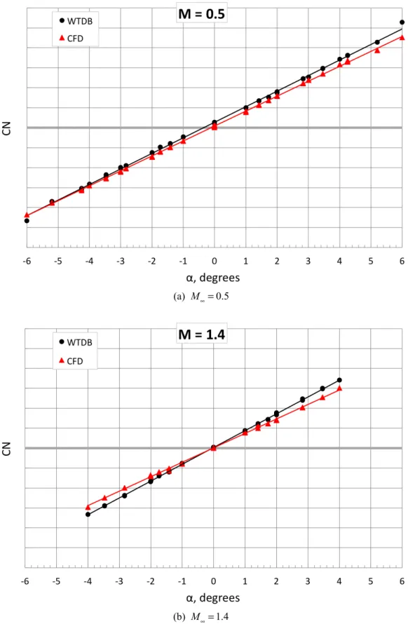
Typical examples of the fits are given in Fig. 3 for M_∞=0.5,1.4, 3.0. Since the data are sensitive, it was necessary to omit the ordinate scale for general publication. The results of Fig. 3(a) are typical of the subsonic cases, while the results of Fig. 3(b) are typical of the low supersonic cases. All of the subsonic, transonic and low supersonic cases have very little deviation from linearity for the angle of attack range of ₋4°≤α ≤4°, the range for which the ascent trajectories are designed. For the higher supersonic cases, Fig. 3(c) is a more typical example. It shows some nonlinearity but not enough to make it unusable for comparison purposes. Note that many of the conditions in Fig. 3

(3)

have combined angles of attack and sideslip, thus making it clear that there is no discernable dependence ofC_Nonβ as predicted by SBT.

The C_Nfit coefficients are compared in Fig. 4. Fig. 4(a) gives the ratio of the slopes, C_N

α, showing remarkable agreement for M_∞≤1.1 and M_∞≥2.5 but rather disappointing agreement for the Mach numbers in between. The possibility of wall interference in that Mach region is discussed in Reference 1. But the cause of the lack of agreement has not yet been definitively determined.

Fig. 4(b) gives the differences in the intercept values, showing good agreement for the subsonic and transonic Mach numbers and rather remarkable agreement for M_∞≥1.3.

Side-Force Coefficient

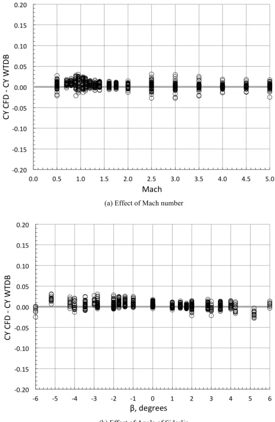
The CFD minus WTDB results for C_Y are given in Fig. 5 to the same scale used in Fig. 2. The scatter of the differences is about 1/3 of that observed in Fig. 2 for C_N. This is not too surprising since the side force derivatives with respect to sideslip are roughly 1/3 of those for the normal force with respect to angle of attack. Note in Fig. 1 that the sideslip flow sees a considerably smaller vehicle planform than that of the pitch flow, which sees the core and both SRB planforms. Following the approach used for C_N, the side force coefficient dependence on β is modeled as

C_Y=C_Y

0+CYββ

(2)

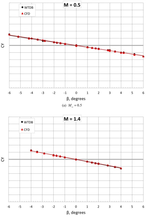
Typical examples of the fits are given in Fig. 6 for M_∞=0.5,1.4, 3.0, using the same (hidden) scale as Fig. 3. Again, all of the subsonic, transonic and low supersonic cases have very little deviation from linearity for the angle of attack range of −4°≤α ≤4°. For the higher supersonic cases, Fig. 5(c) shows some very slight nonlinearity. Also, note again that many of the conditions in Fig. 5 have combined angles of attack and sideslip, thus making it clear that there is no discernable dependence of C_Y on α , as predicted by SBT.

The C_Yfit coefficients are compared in Fig. 7 using the same scales as Fig. 4. Fig. 7(a) gives the ratio of the slopes,

C_Y

β, showing remarkable agreement except for the transonic region, 0.9≤M∞≤1.1. The possibility of wall

interference affecting the WTDB results in this Mach range was discussed in Reference 1. Fig. 7(b) shows that the differences in the fit intercepts are small.

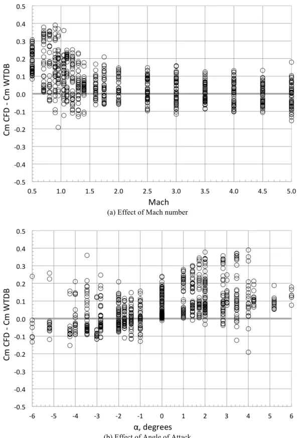
Pitching-Moment Coefficient

The CFD minus WTDB results for C_m are given in Fig. 8. The differences are largest for the subsonic and low supersonic Mach numbers. However, in addition to predicting thatC_Nis linear in α , SBT predicts that the center of pressure for C_N is independent of all three parameters, α,β,M_∞. Hence, SBT would predict C_mto be linear with respect to C_N. Consequently, the following model is used to fit the dependence of C_monC_N:

C_m=C_m

0+

(

xˆCN−xˆBMC

)

CN

(3)

It should be noted that the reference center for the moment coefficients is the balance moment center (BMC) used for the wind tunnel tests1. The BMC is shown in Figure 1 and is located roughly at the location of the force centers of pressure (CP) throughout the ascent trajectory. Hence, the moments are not expected to be large and any movement of the CP, however slight, can contribute to any nonlinearity observed.

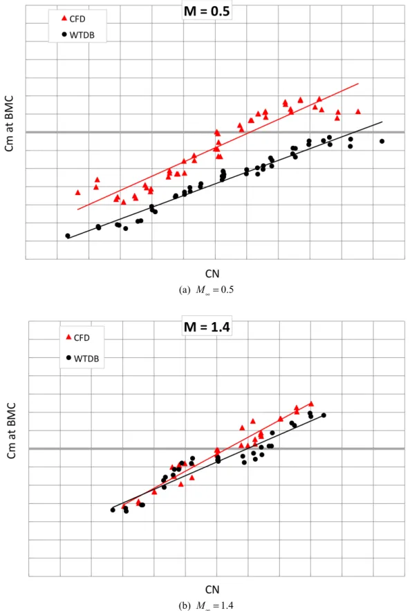
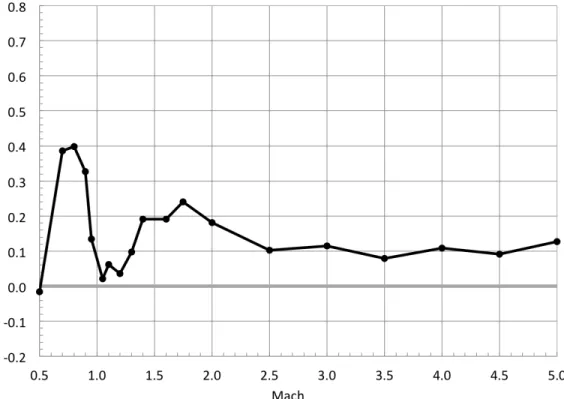
Typical examples of the resulting linear fits are given in Figure 9. The abscissa and ordinate values are omitted to enable publication of the data. The fits are certainly reasonable for comparing the CFD to the WTDB, but nonlinearities are clearly present as well as much more scatter than was seen in the fits for the force coefficients. This is most likely due to the center of pressure being close to the reference center. The fit coefficients are shown in

(4)

Figure 10(a) for the discrepancy inxˆ_C

N and in Figure 10(b) for the discrepancy in Cm0. Except for 0.7≤M∞≤0.9,

the xˆ_C

N discrepancies are quite small.

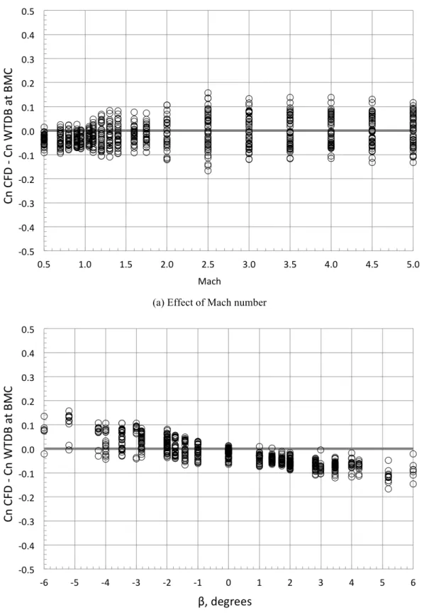
Yawing-Moment Coefficient

The CFD minus WTDB results for C_n are given in Fig. 11 using the scales of Fig. 8. The differences are larger for the higher values of sideslip. Since SBT predicts results forC_nthat are similar to those for C_m, the following model is used to fit the dependence of C_non C_Y:

C_n=C_n

0+

(

xˆCY −xˆBMC

)

CY

(4)

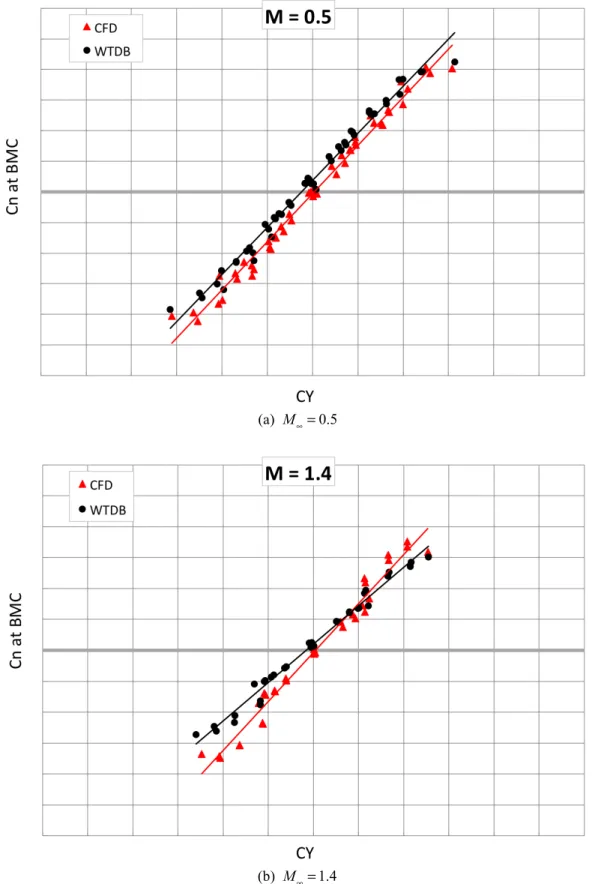
Typical examples of the resulting linear fits are given in Fig. 12. The fits are certainly reasonable for comparing the CFD to the WTDB. Nonlinearities are clearly present but with less scatter than was seen in the fits for the C_m

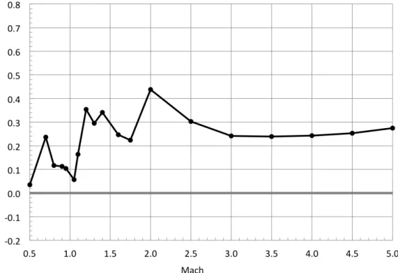
coefficients. This is most likely due to the center of pressure being somewhat farther forward of the reference center compared to the C_mbehavior, as would be expected for the different planforms for each flow. The fit coefficients are shown in Fig. 13(a) for the discrepancy inxˆ_C

Yand in Fig. 13(b) for the discrepancy in Cn0. Except for subsonic

Mach numbers, the xˆ_C

Ydiscrepancy is larger than for xˆCN .

Concluding Remarks

In the opinion of the author, the modeling presented above shows that SBT can be useful for generalizing and comparing the computational and experimental aerodynamic behavior of slender vehicles such as the SLS for conditions during ascent where the angles of attack and sideslip are small. Although it is generally realized that the aerodynamic behavior of slender airplane configurations follows the models used above, it seems less well known that slender airframes, including launch vehicles with boosters and/or fins, behave similarly. In fact, tactical rocket aero design prediction methods based on such behavior have been in use for over 60 years.3-5

Using the SBT models, it is shown that the very-high fidelity RANS results of Reference 2 compare reasonably well with the wind-tunnel-derived database1_{for both the normal and side forces and the locations of their axial centers of} pressure even though the Reynolds numbers are quite different (two orders of magnitude). Reference 2 actually shows that the agreement is within the reported WTDB uncertainties.

Finally, it is expected that additional efforts to locate the regions and causes of the larger discrepancies will help improve future database development, including development of uncertainty models.

Acknowledgements

The author gratefully thanks the SLS Aero Task Team for providing the CFD and WT databases for this analysis. This work was partially funded by NASA Contract NNL12AA09C.

References

1. Pinier, Jeremy T., Bennett, David W., Blevins, John A., Erickson, Gary E., Favaregh, Noah M., Houlden, Heather P., Tomek, William G., “Space Launch System Ascent Static Aerodynamic Database

Development”, AIAA-2014-1254, AIAA 52nd Aerospace Sciences Meeting, National Harbor, MD, January 13-17, 2014.

2. Rogers, Stuart E., Dalle, Derek J., and Chan, William M., "CFD Simulations of the Space Launch System Ascent Aerodynamics and Booster Separation”, AIAA-2015-0778, AIAA 53rd Aerospace Sciences Meeting, Orlando, FL, January 2015.

3. Pitts, William C., Nielsen, Jack N., and Kaattari, George E., "Lift and Center of Pressure of Wing-Body-Tail Combinations at Subsonic, Transonic, and Supersonic Speeds", NACA Technical Report 1307, 1957. 4. Nielsen, Jack N., Missile Aerodynamics, McGraw-Hill, 1960. Reprinted by Nielsen Engineering &

Research, Inc., 1988.

5. Hemsch, Michael J., "Component Build-Up Method for Engineering Analysis of Missiles at Low-to High Angles of Attack", Chapter 4 in Tactical Missile Aerodynamics: Prediction Methodology, Ed. Michael R. Mendenhall, Progress in Astronautics and Aeronautics, Vol. 142, AIAA 1992.

(5)

6. Ashley, Holt, and Landahl, Martin, Aerodynamics of Wings and Bodies, Addison-Wesley, 1965. Reprinted by Dover.

7. Ashley, Holt, Engineering Analysis of Flight Vehicles, Addison-Wesley 1974.

(6)

(a) Effect of Mach number

(b) Effect of Angle of Attack

(7)

(a) M_∞=0.5

(b) M_∞=1.4

(8)

(c) M_∞=3.0 Figure 3. Concluded.

(9)