1
Hypersonic Viscous Flow over Large Roughness Elements
Chau-Lyan Chang* and Meelan M. Choudhari* NASA Langley Research Center, Hampton, VA23681
Originally AIAA Paper 2009-0173, submitted for Theoret. Comput. Fluid Dynamics, special issue for global instability
Viscous flow over discrete or distributed surface roughness has great implications for hypersonic flight due to aerothermodynamic considerations related to laminar-turbulent transition. Current prediction capability is greatly hampered by the limited knowledge base for such flows. To help fill that gap, numerical computations are used to investigate the intricate flow physics involved. An unstructured mesh, compressible Navier-Stokes code based on the space-time conservation element, solution element (CESE) method is used to perform time-accurate Navier-Stokes calculations for two roughness shapes investigated in wind tunnel experiments at NASA Langley Research Center. It was found through 2D parametric study that at subcritical Reynolds numbers, spontaneous absolute instability accompanying by sustained vortex shedding downstream of the roughness is likely to take place at subsonic free-stream conditions. On the other hand, convective instability may be the dominant mechanism for supersonic boundary layers. Three-dimensional calculations for both a rectangular and a cylindrical roughness element at post-shock Mach numbers of 4.1 and 6.5 also confirm that no self-sustained vortex generation from the top face of the roughness is observed, despite the presence of flow unsteadiness for the smaller post-shock Mach number case.
I.
Introduction
iscous flow over discrete and/or distributed surface roughness in hypersonic boundary layers poses a computationally challenging problem, which has significant practical implications in the context of aerothermodynamic predictions for almost all hypersonic vehicles. While it is known that surface roughness causes premature laminar-turbulent transition, a robust transition prediction capability for such flows is currently lacking. For this reason, empirical correlations based on wind tunnel tests and sparse flight data are generally used to estimate transition in the presence of surface roughness. The need for the development of physics-based transition prediction methods was highlighted by the protruding gap filler during shuttle mission STS-114, which led to a space walk by Astronaut Robinson for its removal due to the associated uncertainty in boundary-layer transition and the related impact on the aerothermodynamics of the vehicle. To help develop physics based prediction tools for future hypersonic vehicle design, a combination of detailed measurements and higher fidelity numerical computations of viscous flow over large roughness elements is needed at this time. In particular, current Navier-Stokes computational tools must be improved both in accuracy and robustness in order to perform time accurate computation of hypersonic viscous flows.
Depending upon its size and shape, a discrete roughness element may influence a laminar hypersonic boundary layer in different ways. In the present study, we focus on roughness heights that are comparable to the thickness of the approaching boundary layer. Typical roughness shapes (both that occur naturally and those studied in controlled wind tunnel experiments) cannot be easily simulated with structured grid codes. Therefore, unstructured grid codes are to be preferred for the present application. Roughness introduces flow separation both ahead of and behind the
* Aerospace Technologist, Computational Aerosciences Branch, email: [email protected], [email protected]
V
roughness element, with a complex pattern of accompanying shocks that interact with the boundary layer and the bow shock emanating from the nose. The reverse flow regions may give rise to absolute or convective instability at large enough roughness heights, resulting in a spontaneously unsteady flow and transition in the wake of the roughness site. At low speeds, a rectangular roughness element brings about vortex shedding downstream. This phenomenon is well known and has been documented in the literature. For example, in ref. [1], it was observed and measured experimentally that at large Reynolds numbers in the turbulent regime, flapping and strong vortex motion can originate from both the top and the side faces of the rectangular prism, resulting in sinuous or varicose modes in the wake region. In contrast, flow physics around large roughness elements immersed in supersonic or hypersonic boundary layers is relatively less understood due to limitations in instrumentations and flow visualization techniques. However, Demetriades [2] investigated transition induced by discrete trips in hypersonic boundary layers at Mach number of 3, 7, and 8. It was found that a wedge height several times the boundary layer thickness is required to trip the boundary layer.
While simple roughness shapes can be handled with existing structured mesh computational tools, more complex roughness shapes of practical importance may cause difficulties in grid generation. For this reason, some researchers have used the immersed boundary formulation in conjunction with existing time-accurate compressible Navier-Stokes solvers to handle the roughness geometry [3, 4]. While such an approach may be implemented in existing structured mesh codes, it could encounter difficulties in dealing with complicated shock patterns arising from the interaction of complex roughness geometries with the boundary layer flow. The roughness height being simulated is relatively small in these computations due to the limitation in handling complex shock patterns of the underlying high-order schemes embedded in these Navier-Stokes solvers. In principle, an unstructured mesh could also save computational time by eliminating unnecessary grid clustering near the block interfaces as mandated by topological connectivity. Most existing unstructured mesh CFD codes are based on well-known upwind schemes that utilize a 1D approximate Riemann solver at cell interfaces. Unique flow dependent variables determined by the Riemann solver are required at these cell interfaces to integrate the governing conservation laws over the discretized domain. When applied to multi-dimensional flows, such one-dimensional approximations give rise to undesired numerical issues, especially for triangular or tetrahedral unstructured meshes [5]. For hypersonic applications, carbuncle phenomenon takes place near the blunt nose region [6] and accurate computation of viscous flows with tetrahedral meshes remains a challenge [7]. Remedies for these numerical issues have been proposed and investigated but in general, lack robustness.
A time-accurate, unstructured mesh Navier-Stokes solver, ez4d, [8, 9] based on the space-time conservation element, solution element (CESE) method [10, 11] is used in this study to perform both steady state and time-accurate calculations for various roughness shapes and sizes. Unlike conventional upwind methods, the CESE method is a genuine multi-dimensional scheme formulated by enforcing flux conservation in the discretized space and time domain. Integration of the conservation laws is carried out on staggered discretized volumes called conservation elements (CE). Consequently, no interface reconstruction or dimensional-splitting is needed. Flux conservation in space and time offers distinctly better numerical properties, both in terms of boundary condition treatment and temporal accuracy.
The main objective of this paper is to investigate hypersonic viscous flow over a large roughness element using the unstructured mesh space-time CESE method. The primary focus of this paper corresponds to exploring possible absolute instability of a large roughness element at Reynolds numbers well below the range where natural transition due to known instability mechanisms would be expected to ensue. Both steady-state and time-accurate calculations are performed for both 2D and 3D rectangular roughness elements of height comparable to or larger than the boundary layer thickness. The flow conditions are derived from the on-going series of NASA LaRC experiments by P. Danehy and colleagues [12]. These experiments have provided unique flow visualization data pertaining to the vorticity structures induced by roughness elements of various shapes and sizes. Given the scant knowledge base concerning the physical mechanisms underlying roughness effects on transition, such global flow visualization database can add unique value by allowing one to relate the measured flow structures in the roughness wake to those obtained from unsteady flow computations.
In the following section, a brief description of the numerical method used is given, followed by a grid sensitivity and temporal accuracy study. In the Results and Discussion section, the focus is on three topics: 1) parametric study for vortex shedding behind a 2D roughness element, 2) 3D rectangular prism roughness, and 3) cylindrical roughness element. A brief summary is given at the end.
3
II.
Numerical Method
Three-dimensional compressible Navier-Stokes equations in vector form can be written as
)
1
(
z
H
y
G
x
F
K
z
H
y
G
x
F
t
Q
v v v
where the dependent variable vector is defined as Q = (ρ, ρu, ρv, ρw, e) and x, y, z, and t represent spatial coordinates and time, respectively. Flow variables ρ, u, v, w, and e represent density, three velocity components, and total energy (
e
p
/(
1
)
(
u
2
v
2
w
2)
/
2
), respectively. Definitions of the inviscid flux vectors F, G, H and viscous flux vectors Fv, Gv, Hvcan be found in standard text books and will not be included here. The sourcevector K contains all external forcing or other energy-related source terms. For axisymmetric flows, H = Hv= 0 and
K contains extra terms associated with the cylindrical coordinate system. The Euler equations are recovered by neglecting all viscous and source terms on the right hand side of the equation. To close the system, the perfect gas relation,
p
RT
is used in conjunction with eq. (1).The space-time CESE method is formulated in the strong form of the flux equations. The space-time flux
h
is defined as:)
2
(
)
,
,
,
(
F
F
G
G
H
H
Q
h
v
v
vBy using Gauss’ divergence theorem in the space-time domain, eq. (1) is rewritten in the following integral form
)
3
(
0
v ) (
h
d
s
K
dV
V S
where the space-time flux vector is integrated over the surface S of an arbitrary space-time volume V. The surface normal vector is defined by
s
n
dA
, wheredA
is the area increment on S, andn
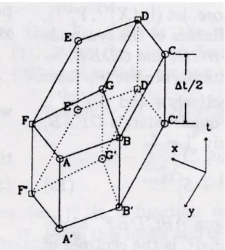
is the outward unit normal vector. Equation (3) is quite general, and in fact, any conservation law with or without a source vector can be cast into this form. Thus, the numerical algorithm devised for eq. (3) can be easily extended for other physical problems. The space time CESE method is formulated by enforcing flux conservation over a discretized space-time domain. For the triangular element shown in Fig. 1, numerical solution of the dependent variables within the triangular element BDF is assumed to satisfy the following first order equation:)
4
(
)
(
)
(
)
(
)
,
,
(
x
y
t
Q
0Q
t
t
0Q
x
x
0Q
y
y
0Q
t
x
y
where Q0 is the solution vector at the solution point O. The vectors Qt, Qx, Qy, and Qz are analogous to the
derivatives of the dependent variables. In contrast to the conventional unstructured mesh method, flux integration is carried out not on the triangular element directly. Instead, three conservation elements (quadrilaterals GBCD, GDEF, and GFAB) around three neighbors are used for the integration of the conservation laws. In the space-time domain, these three quadrilateral CEs extend to three quadrilateral prisms. The solution point O is defined as the geometric center of three conservation elements, ABCDEF. the discretized flux equation for all three prisms can be simplified to
)
5
(
)
(
A
1
A
2
A
3Q
0
I
1
I
2
I
3
K
vwhere A1, A2, and A3 are the surface areas of GBAF, GFED, and GDCB, respectively. Discretized integrals I1, I2,
and I3 are flux integrals for outer-side and bottom faces for three surrounding elements. Source terms in eq. (3) can be integrated to form Kv. Semi-implicit treatment of this source term is usually done to improve solution accuracy
and avoid stiffness issues in reacting flows [8]. Equation (5) is an algebraic equation and can be solved easily without any matrix conversion. The use of eq. (4) results in a formally second-order accurate scheme.
In the above discretized equation, flux integrations are carried out on all faces of the conservation elements shown in Fig. 1(b). Flux vectors are evaluated at faces AB, BC, CD, DE, EF, and FA in the integrals I1, I2, and I3. These faces reside over the smooth regions of all three neighboring elements. As a result, flux vectors are uniquely defined in the discretized equations, no exact or approximate Riemann solver is needed. In light of all the numerical issues associated with the multi-dimensional upwind methods, this distinct feature of the CESE method offers a numerical framework that is superior to other methods in terms of the flux conservation properties in the discretized domain. The derivatives Qt, Qx, and Qy, in Eq. (4) are yet to be determined. In the non-dissipative a-scheme, these
derivatives are computed by solving two remaining flux equations (in addition to the summation of all three conservation elements, Eq.(5)) in conjunction with the following equation:
K
BQ
AQ
Q
t
x
y
where A and B are the Jacobian matrices of the flux vectors F and G, respectively. Thus, there are a total of three equations for three unknowns. Unfortunately, the a-scheme is only neutrally stable for the nonlinear Euler and Navier-Stokes equations and cannot be used in general. Nevertheless, the formulation of such a dissipation-free scheme serves as a baseline to gauge how much numerical dissipation is being added in the dissipative scheme used in Euler or Navier-Stokes equations. In practice, derivatives are evaluated by using solution variations around three neighbors. In the original CESE method, three neighboring solution points are used to obtain three sets of Qx, and
Qy. The unique values are determined by applying a weight average over three sets of derivatives. The weighted
average helps to eliminate oscillations around flow discontinuities. While this approach works fine for relatively uniform meshes, numerical problems arise for highly non-uniform mesh where the triangles used for derivative evaluation are inconsistent with the CE faces. The edge-based derivative approach suggested in ref. [9] modifies the derivative evaluation procedure to remedy the above shortcomings. In this approach, the three vertices of the triangular elements with dependent variables evaluated by using three neighboring solution elements are used to obtain three sets of neighboring derivatives. The same weighted average procedure is then used to uniquely determine the derivatives. There are several weighted average procedures suggested by Chang [11, 13]. In this paper, the second weighting function described in ref. [13] is found to be the most effective and robust. The weighted average is analogous to flux limiters used in conventional upwind schemes. However, it should be noted that in the CESE method, one universal weighted average works for all problems. No tuning for shocks or stagnation regions is necessary.
G F A B C D E O (x0,y0, t0)
Figure 1. Conservation elements for a 2D triangular mesh: (a) top view (b) space time CE volume
5
The above derivation is valid for 2D triangular elements but it can be extended easily for 3D equations. There are questions often raised concerning the fact that a picture of 3D conservation elements similar to that shown in Fig. 1 for 2D cases cannot be drawn. In practice, the CE manifolds need not to be drawn for 3D solutions. As long as the physical time is uniquely defined on each CE faces in the flux integration procedure, it is irrelevant how these CE manifolds look in a four-dimensional space. Both hexahedral and tetrahedral meshes are used in the present study for hypersonic viscous flow computations.
The other issue often raised concerns the fact that for the CESE method, numerical dissipation increases significantly when the CFL number is decreased. For this reason, steady state calculations are done by using local time-stepping, i.e., constant CFL number for all elements. Normally, a CFL number as close to one as possible is used to ensure accuracy. For time-accurate calculations, a constant time step implies that the CFL number varies substantially over the domain if a highly non-uniform mesh is used. The Courant number insensitive (CNI) method [13] should be used to avoid excessive numerical dissipation in the coarse mesh region. For the edge-based derivative approach, the vertices used for derivative calculations are pushed away from the solution point to increase numerical dissipation and pushed inward to reduce the dissipation. A parameter σ is used to control numerical dissipation. An σ value of 1 means zero dissipation. In a CNI scheme, the σ value is very close to 1 in the coarse grid region and increases to a larger value (around 1.3~1.5 for subsonic flows, and 5 or higher for supersonic flows with shocks) maintain numerical stability in the highly stretched mesh inside the boundary layer. As will be shown later, the CNI scheme plays an important role in unsteady calculations.
III.
Grid Sensitivity and Temporal Accuracy Using CNI
Grid Sensitivity Study
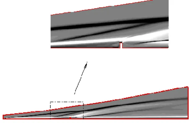
In preparation for time-accurate fine-resolution 2D and full 3D calculations, grid sensitivity study is performed for a simplified 2D roughness at conditions similar to follow-on wind tunnel experiments described in [12]. A Mach 9.65 flow approaches a flat plate at an angle of attack equal to 10 degrees. The post shock Mach number is 6.515. The free stream temperature is 53.3 K and the unit Reynolds number is 3.513 x 10⁶ per meter. The wall temperature is 308 K, which amounts to a ratio of about 0.34 with respect to the adiabatic wall temperature at the post shock condition. The triangular mesh along with the free-stream conditions is shown in Fig. 2, wherein the roughness element is centered on x = 0. The coordinates shown are in mm, which will be used as the unit throughout this paper. There are about 497,000 triangular elements in the planar mesh. Both the boundary layer and the inviscid regions are well-resolved. The numerical Schlieren picture based on the computed base flow solution is shown in Fig. 3. The roughness causes the flow to separate both ahead of and behind the roughness element. The streamwise velocity contours along with streamlines near the roughness location are shown in Fig. 4. The elongated separation region also modifies the effective viscous body shape and in turn leads to a secondary shock. Interaction of this secondary shock with the primary shock causes the merged shock to tilt slightly downward towards the test surface.
Figure 2. Mesh and free-stream conditions for a 2D rectangular roughness element (h = 2 mm).
Figure 3. Computed Schlieren image, including an enlarged view near the roughness.
The theoretical numerical stability limit of the CFL number for the CESE method is one. The higher the CFL number, the more accurate (less numerical damping) the solution is. The numerically converged flowfield shown here was calculated by using local time stepping with a CFL number of around 0.8.
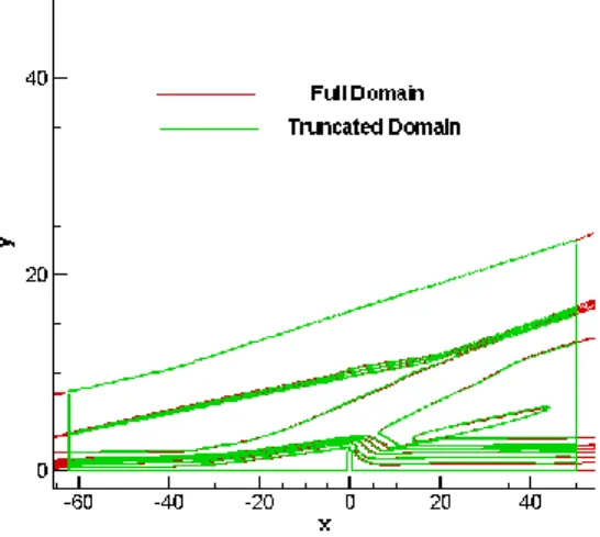
In the above computations, a very fine mesh along the wall-normal direction was used to insure proper initial growth of the boundary layer near the leading edge. As a result, very high aspect ratio meshes must be employed near the inflow boundary. One way to avoid the potential side effects (e.g. very small time step) of such a mesh on time accurate solutions is to start the time accurate computation sufficiently downstream of the leading edge, where both the shock and the boundary layer have already settled down and the peak grid aspect ratios are lower than those near the leading edge. To verify the accuracy of the solutions obtained in this manner, a truncated streamwise domain of x = [-62, 44]from the full domain shown in Fig. 2 was also used for calculations at the same free-stream conditions. The converged solution obtained from the full domain simulations was specified as the inflow profiles at x = -62. The computed solution for this truncated domain is compared to the full-domain solution in Fig. 5. Almost no visible difference exists between these two sets of solutions. Therefore, to save computational time and to avoid high aspect ratio meshes, 3D computations performed herein will be initiated at a location downstream of the leading edge.
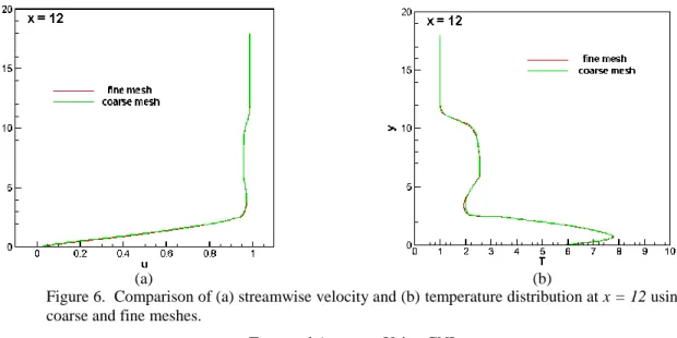
For grid sensitivity study, we generated a coarser mesh with 254,000 triangular elements, i.e., approximately one half the number of cells as those used for the baseline computation in Fig. 2. The computed streamwise velocity and temperature profiles in the wake region are compared at x = 12 in Figs. 6. For the most part, only very small differences are observed between the coarse and fine meshes. Although not shown here, agreement at other locations is also very good. Therefore, the grid size used in the coarse mesh appears to be appropriate to resolve the flow around the selected roughness elements.
As a first step in assessing the effect of roughness height, we compute a similar case that corresponds to ¼ of the roughness height considered in Fig. 2. The computed Schlieren picture for the smaller height configuration is shown in Fig. 7. In comparison with Fig. 3, the shock structure is quite different. Because the upstream separation region is now diminished in extent, the secondary shock does not form until very close to the roughness. Furthermore, the secondary shock is weaker and, therefore, has a weaker effect on the primary shock. Figure 8 shows the streamline patterns and streamwise velocity contours corresponding to the flow in Fig. 7. The front side separation bubble is now substantially smaller than in Fig. 4. Indeed, the back side separation region appears to be larger than the front side. Grid sensitivity study similar to the one discussed for the larger roughness height has also been performed using approximately one half of total number of mesh points. Again, negligible differences were noted between the fine and coarse mesh solutions.
Figure 5. Comparison of Mach number contours for full and truncated domain.
Figure 4. Streamwise velocity contours and streamline patterns for the front and back separation regions.
7
Temporal Accuracy Using CNI
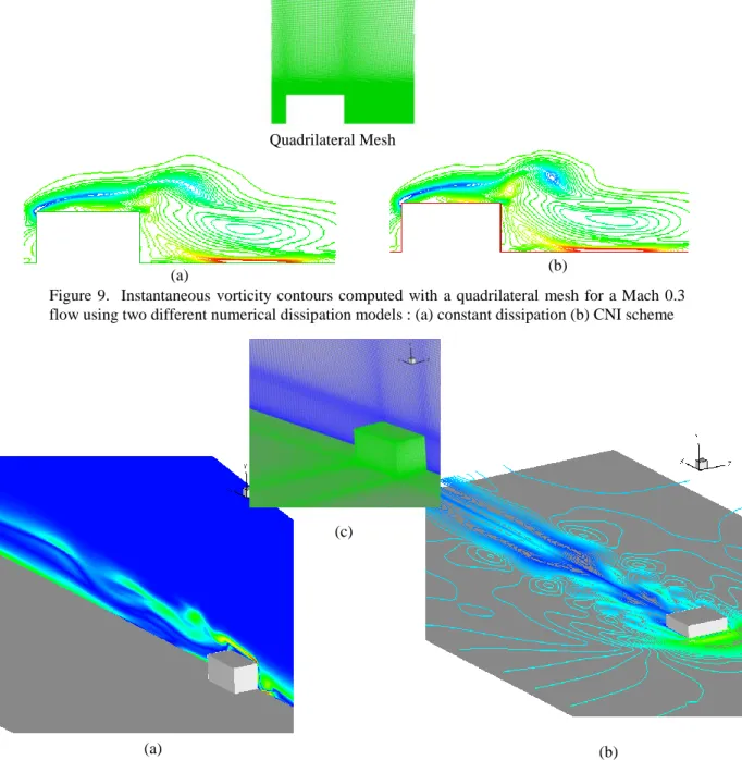
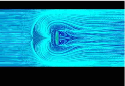
The CNI scheme is important for time-accurate viscous calculations because of the large disparity in grid sizes to resolve the boundary layer. To assess its effect for roughness elements calculations, a Mach 0.3 flow over a rectangular shape roughness is used as a test problem. Free stream temperature is 300 K and adiabatic wall boundary condition is used. A subsonic Mach number is selected here in order to study temporal accuracy when large disturbances and vortex shedding are present in the flowfield. Figure 9 shows computed vorticity contours at one time instant near the roughness element using both CNI and a constant dissipation parameter of σ = 1.9. A quadrilateral mesh with proper resolution inside the boundary layer is also shown in the figure. The CNI scheme leads to considerably crisper vorticity structure than those obtained with a constant dissipation. These results illustrate that the CNI scheme should be used to reduce numerical dissipation for time-accurate calculations. For all unsteady calculations shown in this paper, the CNI scheme is always used. To further assess the CNI scheme for 3D calculations, a hexahedral mesh generated by using the 2D quadrilateral mesh as the baseline is used to compute the same Mach 0.3 flow over a cubic roughness element. The resulting vorticity magnitudes at one time instant after the vortex shedding is established are shown in Fig. 10 along with a close-up view of the mesh. It shows that vortex shedding is well captured for 3D calculations.
Due to difficulties in generating an appropriate viscous mesh with most grid generation software, a normal practice
Figure 6. Comparison of (a) streamwise velocity and (b) temperature distribution at x = 12 using coarse and fine meshes.
(a) (b)
Figure 8. Streamline pattern and streamwise velocity contours for a smaller roughness height (h=0.5 mm).
Figure 7. Numerical Schlieren picture for a smaller roughness height (h = 0.5mm).
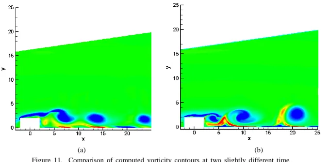
has been to slice a structured quadrilateral or hexahedral mesh into triangles or tetrahedrons. The 2D quadrilateral mesh shown above is sliced into triangles. Consequently, the number of elements doubles but computations per element decrease because of fewer neighboring elements. Overall computational effort is only increased by about 57% for the above mesh (55,000 quadrilaterals and 110,000 triangles). For the CESE method, non-dissipative schemes can only be constructed for a triangular or tetrahedral element. In contrast, discretized equations for a quadrilateral or hexahedral element always have intrinsic numerical dissipation. Thus numerical dissipation and solution accuracy can be better controlled using a triangular or tetrahedral mesh. Computed vorticity results clearly confirm that a triangular mesh gives sharper resolution. Figure 11 shows representative vorticity contours from both meshes at two slightly different time instants. The triangular mesh gives better resolution of the vorticity contours. The spinning of vortices and positive/negative (red/blue) paring are more clearly defined when a triangular mesh is used. For the parametric study discussed in the next section, a triangulated structured mesh is used throughout.
Figure 9. Instantaneous vorticity contours computed with a quadrilateral mesh for a Mach 0.3 flow using two different numerical dissipation models : (a) constant dissipation (b) CNI scheme
(a) (b)
Quadrilateral Mesh
Figure 10. Instantaneous vorticity contours computed with a hexahedral mesh for a Mach 0.3 flow over a cubic roughness element: (a) symmetry plane (b) y = 0.8 plane (c) mesh
(b) (c)
9
IV.
Results and Discussion
Based upon the accuracy study, detailed numerical computations were performed for several cases. As mentioned previously, the main objective is to gain knowledge about the flow physics in the presence of roughness elements at subcritical Reynolds numbers (i.e. below the linear stability limit). A key issue is whether absolute instability or strong spontaneous vortex shedding is present at the flow conditions of interest. To this end, 2D and 3D computations were carried out for: 1) parametric study of vortex shedding over a rectangular roughness element 2) hypersonic flow over a 3D rectangular fence 3) similar flow over a 3D cylinder element. Details of computational results and discussion are described in the following three subsections.
Parametric Study of Vortex Shedding over a Rectangular Roughness
Initial attempts at obtaining time accurate solution for 3D trips at high supersonics Mach numbers yielded an almost stationary (time-independent) state. Therefore, it was decided to perform additional parametric computations. Preliminary results based on 2D simulations involving a square shaped, 2D hump for Mach numbers ranging from 0.3 to 2.0 are presented herein. Typically, at subsonic Mach numbers, nearly periodic vortex shedding was observed at large enough Reynolds numbers based on the roughness height. Figure 12 shows a snapshot of instantaneous vorticity distribution near the hump for M=0.3 and M=0.8. Analogous vortex shedding phenomenon has been observed in low-speed experiments as well as computations involving 3D roughness elements [14,15]. On the other hand, while there exist computations of 2D separating flows without humps where spontaneous shedding has been noted in the past [16,17], we were unable to find experiments involving 2D humps wherein similar behavior has been noted. Experiments by Klebanoff et al. [17], for instance, appear to indicate a stationary flow behind shallower 2D humps. While the absence of vortex shedding in their experiment is perhaps caused by the shallower hump geometries (i.e., smaller h/d and correspondingly lower Reynolds numbers based on roughness height), it’s also possible that the self-sustained unsteadiness in the computation may be numerical in nature.
To further understand the nature of the above unsteady behavior, the time history of vertical velocity fluctuation at selected probe locations from (x-xr)/h = 2.5 to 20 are shown in Fig. 12(b) (where xrdenotes the center of the
roughness element) for M = 0.8. The vertical location of each probe corresponds to the height of the hump in all cases. It is seen that despite the relatively long streamwise region covered by the probe locations, each time series indicates the same dominant frequency (i.e., the fluctuations at that frequency are relatively global). In contrast, the corresponding solutions at supersonic Mach numbers of as low as M=1.2 approach a nearly steady behavior, even though the values of Re and h/0.995 are the same for both subsonic and supersonic cases (Fig. 13). Here, 0.995
Figure 11. Comparison of computed vorticity contours at two slightly different time instants using two different meshes (a) quadrilateral mesh (b) triangular mesh
denotes the thickness of the unperturbed boundary layer at the roughness location and Re is the Reynolds number based on free-stream velocity and the boundary layer thickness. Although vortex shedding is absent in the supersonic cases, we note that time histories similar to those to in Fig. 12(b) do indicate very weak yet regular oscillations even in the supersonic case (see the large time behavior in Fig. 13(b)). For the Mach 0.3 case, the mean reverse flow region starts from the top roughness face and extends a few roughness widths downstream. The mean reverse flow velocity varies from about -0.01(normalized by the fee-stream velocity) at the top face to about -0.3 downstream. Such a large mean reverse flow in conjunction with periodic velocity fluctuations shown in Fig. 12(b) give good indication that global instability may be present in the subsonic cases.
Figure 12(a). Instantaneous vorticity distribution behind a square shaped hump at M = 0.3 and 0.8 (h/ = 0.75, Red = 1200, where 0.995 denotes the thickness of the unperturbed boundary layer at the roughness location)
Figure 12(b). Time history of vertical velocity fluctuation at selected probe locations over a streamwise extent of (x-xr)/h = 2.5, 5, 10, 20 for probes 1, 2, 3, and 4.
Figure 12. Flow field near a 2D hump: subsonic Mach numbers
Figure 13(a). Instantaneous vorticity distribution behind a square shaped hump at M = 1.2 and 2.0 (h/ = 0.75, Red = 1200, where 0.995 denotes the thickness of the unperturbed boundary layer at the roughness location)
Figure 13(b). Time history of vertical velocity fluctuation at selected probe locations over a streamwise extent of (x-xr)/h = 2.5 to 20. The vertical location of each probe corresponds to the height of the hump, and each time series has been separately shifted in the vertical direction in order to allow visualization of multiple time series on the same plot.
Figure 13. Flow field near a 2D hump: supersonic Mach numbers
M = 1.2
11
Hypersonic Flow over a Rectangular Fence
Supersonic flows past a rectangular fence and a cylindrical roughness element under two of the experimental conditions from NASA Langley’s Wind Tunnel experiments (follow-on of ref. [12]) were selected for full 3D computations. In both conditions, the free-stream Mach number is 9.65 and free-stream temperature is 53.3 K. Pure Sutherland law is used for all computations presented herein. The free-stream unit Reynolds number is 3.513 x 10⁶ per meter, which is calculated based on an estimate of the post-shock Reynolds number from the experiment [12]. The unit Reynolds number would be slightly higher if the viscosity is calculated by Sutherland law using the experimental stagnation conditions. The wall temperature is 308 K. The only difference between two different wind tunnel conditions is the angle of attack, which is 10 or 20 degree for Conditions I and II, respectively. The corresponding post-shock Mach numbers are 6.52 and 4.16, respectively. The roughness height is fixed at 2 mm for both the rectangular fence and the cylinder. Thus the roughness height Reynolds number based on the post shock conditions is 10,600 and 6800 for Conditions I and II, respectively. The ratio of roughness height to boundary layer thickness is estimated to be about 0.82 and 1.3, under Conditions I and II, respectively. Such roughness height is relevant for many hypersonic applications. The Reynolds number is about 3.84 x 10⁵ and 2.6 x 10⁵, respectively at the roughness center. The width of the rectangular fence is 8 mm and the diameter of the cylinder is 4 mm.
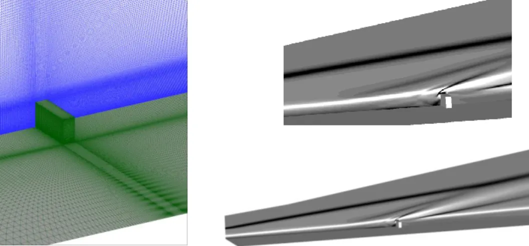
Based upon the grid sensitivity results shown above, we constructed a 3D tetrahedral mesh by stacking up the coarser 2D mesh over a rectangular prism roughness element with a height of 2 mm. Due to the lack of a robust tetrahedral grid generator available, the mesh was obtained by slicing the corresponding hexahedral mesh generated as a multi-block structured grid. The streamwise clustering near the edges of the roughness is an outcome of the topological requirements for the viscous layer near the block interfaces. To save computational time, the inlet of the 3D mesh is located not at the leading edge but at x = -61.5 (see Fig. 2). The center of roughness elements (for both rectangular prism and cylinder to be discussed in the next subsection) is located at x = 0. The computational domain extends to about 50 mm downstream. The converged 2D solutions obtained by the triangular mesh are imposed as the inflow boundary conditions. Two spanwise planes at z = 0 (located at the spanwise center of the roughness) and z = 20 (about 2.5 times the roughness width) are treated as symmetry planes. Based on the good comparisons shown in the previous section, we consider this 3D mesh fine enough to adequately resolve both the inviscid and viscous regions. There are a total of about 26.5 millions tetrahedrons, which is roughly six times the original multi-block structured hexahedral mesh. Fewer elements are needed for the same solution accuracy if the mesh is generated by a truly unstructured grid generator. Figure 14 shows the mesh distribution on the viscous surface and the roughness center symmetry plane.
Figure 14. Close-up of the surface and symmetry plane tetrahedral meshes for the 3D rectangular prism roughness.
Figure15. Numerical Schlieren picture at the symmetry plane for a rectangular prism at Condition I, enlargement near the roughness is also shown.
For all calculations presented herein, local time-stepping iteration was first performed for faster flowfield development. Time-accurate computation with a constant physical time step is then turned on using the CNI scheme to assure better time accuracy. Several time-history probes in the flowfield are monitored in the calculations to ensure either steady-state or quasi steady-state has been reached. Five representative probe coordinates and locations are summarized in Table 1.
Table 1. Coordinates and locations of the probe points
Probe x y z Location
P0 -3.61 0.64 0.16 Front side separation region P3 3.16 0.92 0.16 Right behind the roughness P4 11.18 1.68 0.16 Near wake
P5 30.56 1.70 0.16 Middle wake P12 47.69 1.72 1.90 Far wake
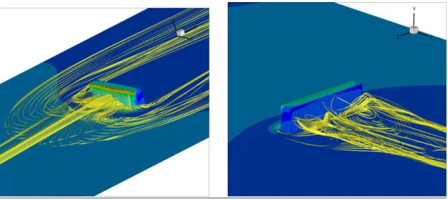
For Condition I, the flow eventually settles to quasi steady state with very small scale oscillations. Figure 15 shows the resulting numerical Schlieren picture at the z = 0 symmetry plane. Similar elongated front side separation as in 2D results develops on the symmetry plane. In addition to the free-stream shock, additional discontinuities are formed above the front-side separation region, on top of the roughness, and in the wake region. The computed surface limiting streamline distribution shown in Fig. 16 exhibits a complex pattern both in the forward and backward separation regions. The zone of influence of the roughness element extends throughout almost the entire spanwise domain, which is five time the roughness width. The streamline patterns within the separation regions are shown in Fig. 17. The horse shoe vortex originated from the front side separation region spirals around the roughness element. Its strength appears to decay downstream as the vortex passes the lateral sides of the roughness. Interestingly, streamlines from the front side separation region do not enter the back side separation region and stay mainly outside of the wake.
Figure 16. Computed surface limiting streamline patterns for the rectangular prism roughness under Condition I
13
To better visualize the wake development, spanwise distribution of streamwise velocity contours are plotted at four streamwise locations downstream of the roughness in Fig. 18. These four planes are located at various distances from the roughness. In the near wake region (x = 2.5 and x = 5), signature of the rectangular roughness is clearly visible. The separated flow (corresponding to negative streamwise velocity) region diminishes downstream and the flow is apparently reattached at x = 25. In the far wake region, the contour exhibits a bulge shape with small valleys on both sides.
Time history of the streamwise velocity and pressure at the above-mentioned five probe points is shown in Fig. 19. The absolute value of time is irrelevant in these calculations. At all five probe locations, the flow has converged to steady state. However, weak oscillations not visible in the scale still exist in most probe locations.
The same rectangular roughness at Condition II is computed using the same tetrahedral mesh. The computed numerical Schlieren at the symmetry plane is shown in Fig. 20. The flow field is quite similar to that under Condition I, except the free-stream shock is slightly closer to the surface. The computed surface limiting streamline pattern is compared with experimental oil-flow visualization in Fig. 21. Reasonable qualitative agreement is
Figure 17. Streamline patterns for rectangular prism roughness under Condition I, showing streamlines originating from (a) front side (b) back side of the separation region and pressure contours on the roughness surface.
(a) (b)
Figure 18. Streamwise velocity contours in a constant-x spanwise plane at four different locations downstream of the wake for rectangular prism roughness under Condition I.
evident. This pattern also appears to be similar to that for Condition I; however, the front side separation region extends slightly further upstream. Again, the domain of influence extends substantially in the spanwise direction. During the initial stage of the time-accurate calculations, the limiting streamlines show a wavy pattern in the wake region. However, these wavy patterns disappear at larger time.
Figure 22 depicts the vorticity magnitude contours on a vertical plane at y = 1. The vorticity pattern behind the roughness element appears to be quite stationary as compared to that shown in Fig. 10 where vortex shedding takes place at low speeds. Vorticity patterns at other y planes across the roughness height indicate that no visible large vortex shedding from the top face of the roughness element is present. However, some small-scale vortical
Figure 19. Time history of (a) streamline velocity and (b) pressure at five different probe locations given in Table I for rectangular prism roughness under Condition I.
(a) (b)
Figure 20. Numerical Schlieren picture at the symmetry plane for a rectangular prism at Condition II, enlargement near the roughness is also shown.
(a)
(b)
Figure 21. Comparison of computed surface limiting streamline with experimental surface oil flow patterns for the rectangular prism roughness under Condition II (a) numerical computation (b) experiments [12].
15
structures are observed in the vicinity of the lateral faces of the roughness element inside the boundary layer (see Fig. 22). Similar to the results from the above 2D parametric study, vortex shedding from the top face of the rectangular prism does not happen under these supersonic conditions. It remains to be seen whether some waviness in time histories (see below) and small vortical structures around the lateral faces are related to any instability mechanism at all. The streamwise velocity distribution at several wake locations shown in Fig. 23 exhibits a distinct mushroom-like structure near the end of the computational domain, which is considerably weaker under Condition I (see Fig. 18). From a stability stand point, such velocity distribution is likely to bring about strong shear-layer instability in the cross plane [18].
Time history of streamwise velocity and pressure at the five probe locations for Condition II is shown in Fig. 24 Unlike in Condition I, both velocity and pressure signals do not converge to a steady state. The initial large oscillations gradually disappear. However, noticeable oscillations are still present. There appears to be a longer scale riding on top of small-scale oscillations. Whether or not the flow would approach a quasi steady state eventually requires continuing computations beyond what is shown in the figure. A rough estimate of the short-scale oscillation gives a frequency in the range of 100 kHz. Further analysis is required to see if these oscillations are related to any instability mechanism. For both conditions, no visible large vortex shedding is observed. However, NASA Langley’s wind tunnel experiments at Condition II using planar laser-induced fluorescence (PLIF) [12] indicate large disturbances downstream of the rectangular fence. Though similar phenomena were not found by the present numerical computations, Condition II is apparently more unstable than Condition I owing to the facts that a prominent mushroom shaped structure appears in the wake and some unsteadiness is present in the time history at several probe locations. External forcing, such as the wind tunnel noise, may result in large disturbances development in the wake region if convective instability is indeed the dominant mechanism.
Figure 23. Streamwise velocity contours on a spanwise plane at four different locations downstream of the wake for rectangular prism roughness under Condition II.
Figure 22. Vorticity magnitude contours on y = 1 plane for a rectangular element under Condition II.
Hypersonic Flow over a Cylinder Roughness Element
Parallel to rectangular elements, similar calculations were also performed for a cylinder roughness element with the same 2 mm height and a diameter of 4 mm. A hexahedral mesh with 5.6 million elements (Fig. 25), better suited for parametric study, is used for both Conditions I and II. The computed numerical Schlieren picture and the surface pressure contours for Condition II are shown in Fig. 26 The shock pattern is similar to that for a rectangular fence, except the front side separation region induced shock and the wake region recompression shock are not present. The same five probe points shown in Table I are used to monitor temporal development of the flowfield. Figure 27 compares the time history of pressure signal for both Conditions I and II. The solution converges to a steady-state for Condition I. Similar to the rectangular fence case, some small-scale oscillations persist for Condition II. The signal exhibits multiple frequencies. The dominant one is estimated to be around 50 ~ 70 kHz. Again, further analysis may help clarifying whether these oscillations are indeed instability waves or numerical artifacts due to lack of resolution.
Streamwise velocity contours at various locations downstream of the wake are shown in Fig. 28. Similar to the rectangular fence case, Condition II gives rise to a mushroom-like structure near the end of the computational domain. Such mushroom-like structure implies that for a fence or cylinder roughness height of 2 mm under wind tunnel Condition II, instability wave may be present in the wake region near the center line. Since the square root of the Reynolds number at the roughness location under Condition II is only about 500, the unperturbed boundary layer may just begin to become unstable for second mode disturbances. The instability wave associated with the inflectional mushroom-like structure could be the dominant instability mechanism for breeding large disturbances, which in turn may cause early transition to turbulence downstream.
Figure 24. Time history of (a) streamwise velocity and (b) pressure at five different probe locations given in Table I for rectangular prism roughness under Condition II.
17
Figure 25. Close-up of the surface and symmetry plane hexahedral meshes for the 3D cylinder roughness element
Figure 26. Numerical Schlieren picture at the symmetry plane and surface pressure contours for a cylinder roughness at Condition II.
Figure 27. Comparison of time history of computed pressure signal for cylinder roughness at Conditions (a) I and (b) II.
(a) (b)
Figure 28. Comparison of streamwise velocity evolution downstream of the wake for cylinder roughness element under Conditions (a) I and (b) II.
V.
Summary
The space-time CESE method is used to study hypersonic viscous flow over large roughness elements using unstructured meshes. Both shock-shock and shock boundary layer interactions near the separation region are captured in the computed solution. The multi-dimensional CESE scheme offers a robust numerical method to handle complex shock and viscous flows. In all of the calculations, no tuning to accommodate the shocks was necessary; and grid converged solutions were demonstrated for the 2D case. Both 3D hexahedral and tetrahedral meshes were used to compute steady-state and time-accurate hypersonic flows over a rectangular fence and a cylindrical roughness element. For a post shock Mach number of 4.1 or higher, both 2D and 3D solutions with a roughness height exceeding the boundary layer thickness showed a larger separation region ahead of the roughness element than the one behind. The perturbation induced by the roughness element extends two to three times the roughness width along the spanwise direction. The surface flow pattern agrees reasonably well with available experimental results. Although no large disturbances as seen in the experimental PLIF visualization [12] were found in the computations, flow unsteadiness is observed downstream of the roughness element for both rectangular and cylindrical roughness elements under wind tunnel Condition II, which corresponds to a roughness height of about 1.3 times the boundary-layer thickness. Further computations at larger Reynolds numbers are underway to explore other possibilities of large disturbances development in the wake, including convective instability mechanisms caused by external forcing. A parametric study for a square shaped roughness element using 2D calculations showed a spontaneous onset of vortex shedding for subsonic Mach numbers at Re = 1200. For supersonic
boundary layers, no prominent vortex shedding was observed for the same combination of Reynolds number and ratio of roughness height to boundary layer thickness. In such flows, any large disturbances downstream of the roughness are more likely to be related to the convective instability of the roughness wake. A mushroom like streamwise velocity distribution is found in the wake of the roughness for one of the wind tunnel condition under investigation. Elongated streaks of this kind can sustain stronger instabilities than those of the unperturbed boundary layer [18], potentially causing an earlier transition.
Acknowledgments
The authors thank Scott Brynildsen for generating some of the computational grids used in this work. Assistance by William Jones and Beth Lee-Rausch of NASA Langley Research Center is also gratefully acknowledged.
References
1. Sakamoto, H. and Arie, M, “Vortex Shedding from a Rectangular Prism and a Circular Cylinder Placed Vertically in a Turbulent Boundary Layer,” J. Fluid Mech., Vol. 126, pp. 147-165, 1983.
2. Demetriades, A., “Supersonic and Hypersonic Bounadry-Layer Transition Induced by Discrete Trips,” Boundary Layer Stability and Transitionto Turbulence, FED-Vol. 114, American Society of Mechanical Engineers, New York, 1991, pp. 173–178
3. Duan, L, Wang, X., and Zhong, X., “A High-Order Cut-Cell Method for Numerical Simulation of Hypersonic-Boundary Transition with Surface Roughness,” AIAA Paper 2008-3732, 2008.
4. Marxen, O. and Iaccarino, G., “Simulation of the Effect of a Roughness Element on High-speed Boundary-layer Instability,” AIAA Paper 2008-4400, 2008.
5. Gnoffo, P. A. and White, J. A., “Computational Aerothermodynamics Simulation Issues on Unstructured Grids,” AIAA Paper 2004-2371, 2004.
6. Chauvat, Y., Moschetta, J.-M., and Gressier, J., “Shock Wave Numerical Structure and the Carbuncle Phenomenon,” Int. J. Numeri. Meth. Fluids Vol. 47, No. 8-9 pp. 903-909, 2004.
7. Candler, G. V., Barnhardt, M. D., Drayna, T. W., Nompelis, I., Peterson, D. M., and Subbareddy, P., “Unstructured Grid Approaches for Accurate Aeroheating Simulations,” AIAA Paper 2007-3959, 2007. 8. Chang, C.-L., “Time-Accurate, Unstructured-Mesh Navier-Stokes Computations with the Space-Time
CESE Method,” AIAA Paper 2006-4780, presented at the 42th AIAA/ASME/SAE/ASEE Joint Propulsion Conference and Exhibit, July 10-12, 2006, Sacramento, CA.
9. Chang, C.-L., “Three-Dimensional Navier-Stokes Calculations Using the Modified Space-Time CESE Method,” AIAA Paper 2007-5818, 2007.
10. Chang, S.-C., “The Method of Space-Time Conservation Element and Solution Element–A New Approach for Solving the Navier-Stokes and Euler Equations,” J. Comput. Physics, Vol. 119, pp.295-324, 1995. 11. Chang, S.-C. and Wang, X.-Y., “Multi-Dimensional Courant Number Insensitive CE/SE Euler Solvers for
19
12. Danehy, P.M., Garcia, A.P., Borg, S., Dyakonov, A.A., Berry, S.A., Inman, J.A., and Alderfer, D.W., “Fluorescence Visualization of Hypersonic Flow Past Triangular and Rectangular Boundary-Layer Trips,” AIAA Paper 2007-536, 2007.
13. Sin-Chung Chang, "Courant Number and Mach Number Insensitive CE/SE Euler Solvers," AIAA Paper 2005-4355, presented at the 41th AIAA/ASME/SAE/ASEE Joint Propulsion Conference and Exhibit, July 11-13, 2005, Tucson, AZ.
14. Acarlar, M.S., and Smith, C.R., “A Study of Hairpin Vortices in a Laminar Boundary Layer. Part 1.” J. Fluid Mech., Vol. 175, pp. 1-42, 1987.
15. Tufo, H. M, Fischer, P. F., Papka, M. E. and Blom, K., “Numerical Simulation and Immersive Visualization of Hairpin Vortices,” in Proc. of the ACM/IEEE SC99 Conf. on High Performance Networking and Computing. IEEE Computer Soc., CDROM (1999).
16. L. Pauley, “Response of Two-Dimensional Separation to Three-Dimensional Disturbances,” ASME Journal of Fluids Engineering 116(3): 433-438, September, 1994.
17. Klebanoff, P.S. and Tidstrom, K.D., “Mechanism by Which a Two-Dimensional Roughness Element Induces Boundary-Layer Transition,” The Physics of Fluids, vol. 15, No. 7, pp. 1173-1188, 1972.
18. Choudhari, M., Li, F., and Edwards, J.E., “Stability Analysis of Roughness Array Wake in a High-Speed Boundary Layer,” AIAA Paper 2009-0170, 2009