Aeroelasticity Branch, NASA Langley Research Center, Hampton, VA 23681, USA [email protected], [email protected]
Keywords: Computational Aeroelasticity, Unsteady Aerodynamics, Flutter, Transonic Dip, Aeroelastic Validation, FUN3D, Flutter Bucket.
Abstract:
This paper builds on the computational aeroelastic results published previously and generated in support of the second Aeroelastic Prediction Workshop for the NASA Benchmark Supercritical Wing configuration. The computational results are obtained using FUN3D, an unstructured flow solver developed at the NASA Langley Research Center. Flutter analyses are performed using various aerodynamic models including linear doublet lattice, Euler solutions, Reynolds-averaged Navier-Stokes and Delayed Detached Eddy Simulations. The analyses are performed across the transonic Mach range for a range in angle of attack from 0° to 5◦, with focus on identifying the transonic dips in the flutter onset boundaries.
1 INTRODUCTION
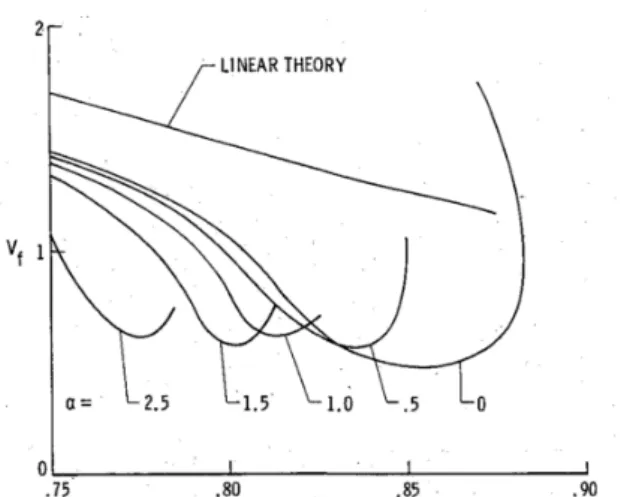
Historically, the prediction of the transonic dip has proven elusive. This remains the case for the Benchmark Supercritical Wing (BSCW). In the seven years since the first Aeroelastic Prediction Workshop (AePW), we have endeavored to evaluate the influences of shock development and separation onset on the aeroelastic characteristics of this wing, with the long-term objective of having demonstrated, reliable, predictive aeroelastic capability throughout the transonic range. The goal of the current work is to develop and understand the bucket in the transonic flutter boundary for this configuration, evaluating the applicability of various levels of aerodynamic modeling for different flow field physics. Historically, the location (in terms of Mach number) and depth (in terms of dynamic pressure or velocity) of the transonic dip have been shown to be functions of the angle of attack. There are many configurations where this behavior has been observed in the technical literature, including both computational and experimental examples. A specific example for the NACA 64 A-010 airfoil is reproduced from reference 1 in Figure 1.
2 BACKGROUND 2.1 The BSCW model
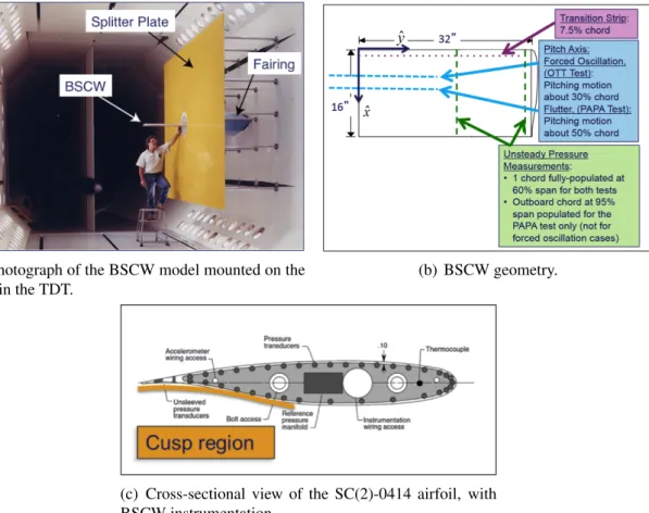
The BSCW model, shown in Figure 2, has a simple, rectangular, 16- x 32-inch wing planform, with a NASA SC(2)-0414 airfoil. It was first tested in the TDT in 1991 [2]. For this test, the wing was mounted on the TDT Pitch and Plunge Apparatus (PAPA) to obtain the flutter boundary at various Mach numbers and angles of attack for this two-degree of freedom system. In 2000, the wing was tested again, this time on an Oscillating Turntable (OTT) [3]. The
Figure 1: Effect of angle of attack on NACA 64 A-010 flutter boundaries; Source: Reference 1, Figure 7.
purpose of the OTT test was to measure aerodynamic response during sinusoidal (forced) pitch oscillation of the wing.
For both the OTT and PAPA tests, the model was mounted to a large splitter plate, sufficiently offset from the wind-tunnel wall (40 inches) to (1) place the wing closer to the tunnel centerline and (2) be outside the tunnel wall boundary layer [4]. The wing was designed to be rigid, with the following structural frequencies for the combined installed wing and OTT mounting system: 24.1 Hz (spanwise first bending mode), 27.0 Hz (in-plane first bending mode), and 79.9 Hz (first torsion mode). When installed on the PAPA mount, the combined system frequencies were 3.33 Hz for the plunge mode and 5.20 Hz for the pitch mode [5]. The plunge and pitch modes are the only modes included in the aeroelastic analyses of the PAPA-mounted configuration to be presented in this paper.
For instrumentation, the model has pressure ports in chordwise rows at the 60% and 95% span locations. For the BSCW/PAPA test, both rows were fully populated with unsteady in situ pressure transducers. The quantitative information obtained consists of unsteady data at flutter points and averaged data on a rigidized apparatus at the flutter conditions. For the BSCW/OTT test, only the inboard row at 60% span was populated with transducers. The quantitative infor-mation for the OTT test consists of unsteady pressure data and accelerometer data for forced pitch oscillations and for the unforced system at stabilized flow conditions.
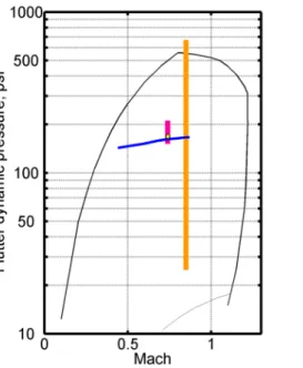
2.2 Summary results from the second Aeroelastic Prediction Workshop
The second AIAA Aeroelastic Prediction Workshop (AePW-2) took place in conjunction with the AIAA SciTech 2016 Conference [6]. The computational aeroelasticity community was chal-lenged to analyze the BSCW configuration at three conditions (M=0.7 atα= 3.15◦on the OTT; M=0.74 atα = 0◦on the PAPA; and M=0.85 atα= 5◦on the PAPA) and to present their results at the workshop. The experimental data from the OTT test indicated that the BSCW exhibited strong shocks and shock-boundary-layer interactions, inducing separated flow at moderate an-gles of attack at transonic conditions [7]. The computations of the transonic flow, in conjunction with the flutter boundary predictions, were therefore the focus of the workshop [8]. The sum-mary of flutter onset predictions from AePW-2 is shown in Figure 3. The predictions at Mach 0.74, 0◦ angle of attack have considerably less scatter than the prediction at Mach 0.85, 5◦ angle of attack. The lower Mach number, lower angle of attack predictions also surround the experimental flutter onset condition,q¯=169 psf.
OTT in the TDT.
(c) Cross-sectional view of the SC(2)-0414 airfoil, with BSCW instrumentation.
Figure 2: BSCW model.
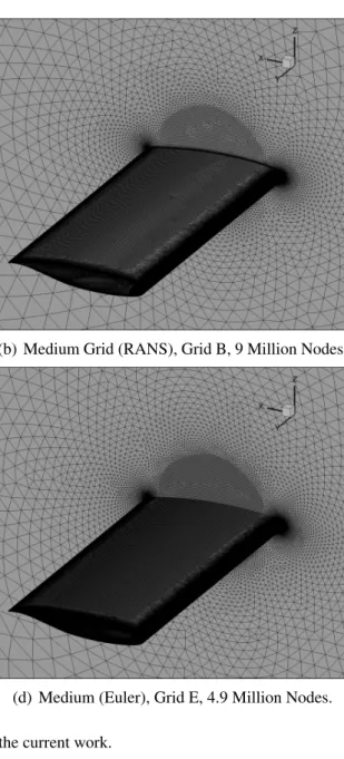
2.3 Grids
For the present study, three of the unstructured grids that are detailed in reference 9 were uti-lized: the coarse, medium and extra fine grids. In the current paper, Grid D is referred to as the extra fine grid. The grid distributions for both the wing surface and the plane of symmetry are presented in Figure 4. Additionally, two grids were generated for use in performing Euler simulations. These grids are also shown in Figure 4.
3 ANALYSIS PROCESSES
Solutions to the Reynolds-averaged Navier-Stokes (RANS) equations were computed using the NASA Langley-developed computational fluid dynamics (CFD) software FUN3D [10]. The flow solutions were produced with turbulence closure obtained using the Spalart-Allmaras (SA) one-equation model [11, 12]. Inviscid fluxes were computed using the Roe scheme [13], pri-marily without a flux limiter. The solutions were produced by running three distinct analyses, differentiated by the treatment of the structure, the initial condition and the temporal parameters. The rigid, static aeroelastic and dynamic aeroelastic solution processes are described below.
3.1 Rigid analysis
The initial solution for each angle of attack at Mach 0.74 was generated for a rigid wing. In general, these solutions were run in a “steady” mode, in which the solutions computed were not time-accurate and the structure was represented as a fixed position outer mold line. The position (angle) was different for each angle of attack and analyzed in an individual simulation. Time
Figure 3: Flutter boundary results from AePW-2.
integration was accomplished by an Euler implicit backwards difference scheme, with local time stepping to accelerate convergence. Although some of the cases were not asymptotically steady, the rigid steady simulation was still the first step performed. The cases that were not asymptotically steady occurred at the higher angles of attack and will be identified as a subset of the results presented. These cases did not converge to a fixed pressure distribution and should be run in a time-accurate manner where the range of the physical solution can be established. Results of time-accurate rigid simulations are not presented in the current paper.
3.2 Unsteady aeroelastic analyses
For aeroelastic analyses, the flow equations were solved in a time-accurate mode [14] coupled with a structural solver, allowing the grid to deform. For this work, this coupling was performed internal to the FUN3D code [15] using a modal representation of the structural dynamics. This modal solver was formulated and implemented in FUN3D in a manner similar to other NASA Langley aeroelastic codes (CAP-TSD [16] and CFL3D [17]). For the BSCW computations presented here, the structural modes were obtained via normal modes analysis (solution 103) with the Finite Element Model (FEM) solver in MSC NastranT M [18]. The modes were then interpolated to the surface mesh using the method developed by Samareh [19]. The BSCW FEM is described in reference 8.
To solve the unsteady flow equations, the FUN3D solver employs a dual-time-stepping method, which is widely used in CFD. This method involves adding a pseudotime derivative of the conserved variables to the physical time derivative that appears in the Navier-Stokes equa-tions. Subiterations are run within each physical (global) time step to converge the flow so-lution. Convergence here refers to the process where the pseudotime derivative vanishes as the subiterations proceed within each physical time step. At the end of the iterative process, a solu-tion to the original unsteady Navier-Stokes equasolu-tions is obtained for that physical time step. For an infinitely large physical time step, the dual-time solver becomes identical to the steady-state solver, though of course, all time accuracy is lost.
(a) Coarse Grid (RANS), Grid A, 3 Million Nodes. (b) Medium Grid (RANS), Grid B, 9 Million Nodes.
(c) ExtraFine Grid (DDES, RANS), Grid D, 35 Mil-lion Nodes.
(d) Medium (Euler), Grid E, 4.9 Million Nodes.
Aeroelastic analysis requires a grid deformation capability. The grid deformation in FUN3D is treated as a linear elasticity problem. In this approach, the grid points near the body can move significantly, while the points farther away may not move at all. For the aeroelastic simulations in this paper, a predictor-corrector coupling method between the flow solution and the structural solution has been used. Within each physical time step, the flow field solution is converged using the subiterations and subsequently coupled with the structural equations. This coupling occurs only once for each physical time step. The coupling is described further and explored in detail in reference 9. Temporal convergence studies are not part of the work presented in the current paper. The current work utilizes the time step size (0.0002 seconds) that resulted from the temporal convergence studies in reference 9. Note that the nondimensional time step size varies slightly for different cases, as the speed of sound varies slightly.
3.2.1 Static Aeroelastic Analysis
The static aeroelastic simulation procedure begins from the last point in the rigid steady solution at identical Mach number and unloaded (rigid) angle of attack. Static aeroelastic simulations are obtained by restarting the CFD analysis from this rigid steady solution. A high value of structural damping (0.9999) is used to allow the structure to find the equilibrium position with respect to the mean flow. The fluid-structure coupling provides a step input to the system, initi-ating the migration from the rigid solution to the coupled static aeroelastic solution. In general, the static aeroelastic analysis is performed using larger time steps and fewer subiterations than have been shown to be required for a time-accurate temporally-converged solution. This issue is briefly explored later in this paper.
3.2.2 Dynamic Aeroelastic Analysis
Dynamic (flutter) analysis is performed in a multistep process, with the dynamic solution started from the static aeroelastic solution at corresponding Mach number, angle of attack and dynamic pressure, and setting the structural damping value to zero. An excitation is provided to the system by adding an initial condition to the generalized (modal) velocities. For most results presented in the current paper, identical values of initial generalized velocity are applied simul-taneously to both the plunge and pitch modes. The exception is when only the pitch mode is included in the analysis, denoted as single degree of freedom or pitch only cases. The effects of the initial excitation value on the flutter solution are discussed in detail in reference [20]. The wing response, in the form of the time varying pitch angle, is computed and a logarithmic decrement method is used to calculate the damping ratio. For a stable solution, the damping ratio is greater than zero, and for an unstable solution, the damping ratio is less than zero. To determine the flutter onset dynamic pressure, linear interpolation is performed to find the zero damping case using the two cases on either side of the stability boundary (that is, using the two dynamic pressures where the sign of the damping changes in between them). The flutter frequency is then calculated using the same interpolation coefficients.
A logarithmic decrement technique, detailed in reference 20, is applied to the time history of the pitch angle displacement for each simulation. The technique performs a linear fit to the logarithm of the extreme values of the oscillation to calculate the system damping.
Figure 5: Flutter Boundary Results using FUN3D from AePW-2 [21].
4 PRIOR WORK
Results and relevant lessons learned from the prior analyses are summarized in this section. The summary results from AePW-2 were shown in Figure 3 for the two flutter test cases: Case #2: Mach 0.74, 0◦ angle of attack and Case #3: Mach 0.85, 5◦ angle of attack. Case #2 was chosen for the workshop because there was a corresponding experimental data set and that data set indicated that the flow was attached, representing a case where most methods should perform well. Case #3 was an optional workshop case that was a carryover from AePW-1, where the results from different analysis teams showed significant scatter in frequency response functions. At this condition, analysis results from the workshop indicated the presence of the shock-induced separated flow dominating the upper surface and the aft portion of the lower surface, making it a very challenging case for RANS simulations. There was no experimental data at this condition for comparison with the computations.
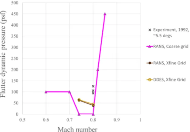
Figure 5a provides a summary of the FUN3D predictions for AePW-2 [21] and graphically illustrates the issues and various solutions associated with computation of the flutter boundary for Case #3. Depending on the grid resolution and the scheme used, the dynamic pressure range is nearly 280 psf in dynamic pressure for the flutter boundary prediction at Mach 0.85. It is because of this very wide range of flutter predictions that we recommended further analysis. Results were generated for AePW-2 to examine the influences of using a flux limiter and grid resolution. Focusing on the Mach 0.85 andα = 5◦ case, the results showed that using a limiter shifts the predicted shock location aft on the upper surface of the wing, affecting the size of the separated region behind the shock [21]. In addition, the grid resolution affects both shock strength and location. As shown in Figure 5, the range of the dynamic pressure between the coarse and fine grid solutions with a limiter is nearly 200 psf. On the other hand, the corre-sponding range for the solutions without the limiter is only about 100 psf. In addition, a DDES solution on a fine grid produced a flutter boundary point in between the coarse- and fine-grid solutions. This very wide range of predictions prompted an attempt to calculate the flutter boundary over a wide range of Mach numbers from 0.6 to 0.85 at5◦ angle of attack, which will be discussed in the following section.
4.1 Continued analyses expanding AePW2 Test Case 3c: Flutter at 5◦ angle of attack, varying Mach number
Computational efforts following the workshop using FUN3D are summarized in reference 9. The wide range of workshop predictions at Mach 0.85, α = 5◦ prompted exploration of the flutter boundary as a function of Mach number at this angle of attack, focusing between Mach 0.6 and 0.85. One speculation was that the wide range was due to some simulations being in the flutter dip, while others were on the back side of the bucket. That is, there could be great sensitivity to very small changes in Mach number or very small changes between the codes’ implementations or inputs.
Calculations using a coarse grid produced a flutter boundary, shown in Figure 6, where analyses at Mach 0.80 and 0.74 were unstable at the lowest non-zero dynamic pressure that was analyzed,
¯
q =25 psf. Lower Mach numbers (0.60 and 0.70) produced a flat portion of the flutter boundary and higher Mach numbers (0.82 and 0.85) indicate the back side of the flutter bucket, as the flutter onset dynamic pressure increased significantly. At Mach 0.85, the influence of the flux limiter was examined and shown to introduce additional damping into the solution and raise the flutter onset condition by 50% (fromq¯=450 psf to 670 psf).
The calculations at Mach 0.74 and Mach 0.8 were repeated using a refined grid, with and with-out the DDES option activated. The calculation with the DDES turned on and off produced identical flutter boundary predictions, q¯= 55 psf at Mach 0.8 and q¯= 68 psf at Mach 0.74. These points are also shown in Figure 6.
Figure 6: Flutter boundary results, URANS,α= 5◦, circa 2017.
4.2 Continued analyses expanding AePW-2 test case 2c: Flutter at Mach 0.74, varying angle of attack
The flutter boundary obtained from RANS analyses of the BSCW indicate that the transonic dip is due to separating/reattaching flow [20]. A critical pitch angle was identified asα = 6.5◦ at Mach 0.74 for the medium grid analyses and a slightly higher critical angle for the extra fine grid analyses. The critical angle is defined here as the pitch angle above which the flow field is significantly and qualitatively different from the flow field at lower angles of attack. Effects of this critical angle are seen in the rigid steady results as a reversal in the shock movement with increasing angle of attack. Pressure coefficients on the wing upper surface at the 60% span station, calculated from rigid steady analyses are shown for angles of attack from0◦ to8◦
(a) URANS steady rigid simulations.
(b) Enlarged view of shock region, comparison with experimental data.
Figure 7: Pressure coefficients on upper surface at 60% span, Mach 0.74, URANS and experiment.
in Figure 7. The results show that the reversal of the shock migration occurs between 6◦ and 6.5◦angle of attack. This figure includes a second plot, which shows a comparison of URANS solutions that correspond to experimental data sets obtained over a reduced range of angle of attack. The URANS solutions consistently locate the shock aft of the experimental data, but the overall shape of the upper surface pressure is well-captured and the trend of the shock moving aft as angle of attack increases betweenα=−1◦and5◦is duplicated. Experimental data is not available at this Mach number at higher angles of attack.
The effects of the critical angle are seen in the static aeroelastic solutions as reductions in the to-tal angle of attack with increasing dynamic pressure when the toto-tal angle of attack exceeds6.5◦. The effects seen in the dynamic aeroelastic solutions are a change in the phase of the frequency response functions of the pitching moment coefficient when the dynamic pressure exceeds the flutter condition. Examination of the dynamic aeroelastic solutions’ shock movement over a cycle showed the same shock position reversal as observed in the steady rigid and static aeroe-lastic solutions. This behavior also led to several frequencies appearing to have significant magnitudes in the frequency response functions. This frequency spread isn’t a superharmonic effect, but rather the effect of separation onset part way through the cycle.
analy-Figure 8: Flutter Boundary Results using Euler Analysis.
ses produced different flutter boundaries when separation onset is part of the flutter inducement (i.e., within the transonic dip region). When separation is not a factor, the RANS simulations indicate that the perturbation level matters little. At Mach 0.74, the transonic dip of the flutter boundary is defined by solutions perturbed such that they reach 6.5◦ total angle of attack. At other transonic Mach numbers, it is anticipated that there are similar critical angles. It is also anticipated that the critical angle of attack will be lower at higher Mach numbers and higher at lower Mach numbers.
5 FURTHER EXPLORATION OF THE FLUTTER BOUNDARY, VARYING MACH AND ANGLE OF ATTACK
5.1 Euler analyses
The RANS predictions have indicated that the depth of the transonic dip for the BSCW is driven by shock-induced separating and reattaching flow. Because Euler equations do not include viscous effects, any transonic dip predicted by Euler analyses would not be due to viscous shock boundary layer interactions producing separating and reattaching flow.
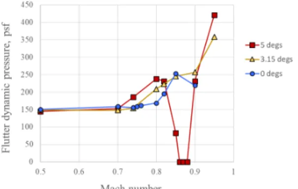
Flutter boundaries for Euler simulations of the BSCW are shown in Figure 8. Theα= 5◦ case has a flutter dip that extends down to, but exclusive of, q¯=0 psf. Atq¯= 0 psf, the coupled fluid-structure system reverts to the behavior of the structural dynamic system with no structural damping; the response is a limit cycle oscillation. For the Euler results, the bucket begins at Mach 0.82, followed by a rapid decrease in stability shown by the simulations at Mach 0.85. The bottom of the bucket, at q¯ = 0 psf, spans from Mach 0.86 to 0.88. Beyond this Mach number, the back side of the bucket rises steeply and the system is stable for high dynamic pressures.
Euler flutter results, presented as damping vs dynamic pressure at Mach 0.87,α= 5◦, are shown in Figure 9. For this case, all of the results are unstable, or neutrally stable in the case ofq¯=0 psf. The damping value doesn’t change significantly if the matched point conditions are used in the analysis or if the limiter is used in the analysis. One case,q¯=100 psf, is shown where only the pitch mode is included in the analysis. Utilizing only this single degree of freedom modifies the values of damping and frequency for this unstable mode by only 13% and 7%, respectively. Thus, atq¯=100 psf, at this Mach and angle of attack, the flutter mechanism is a single degree of freedom flutter. Because the damping and frequency are so similar to the pitch and plunge result for this case, by implication, the other results at Mach 0.87 are also presumed to be single degree of freedom flutter.
Figure 9: Damping of Euler analysis results, Mach 0.87,α= 5◦. (Instability is indicated by a negative value of damping.)
Details of the flutter simulations at a dynamic pressure of 25 psf are examined in more detail. Detailed information was extracted for the flutter solution for 2 cycles. The pressure coefficients at the 60% span are shown in Figure 10a over these two cycles. Each of the grey lines in the plot represent a snapshot of the time history of the pressure coefficient distribution. The pink and blue lines correspond to points in time identified on the time history of the angle of attack, shown in Figure 10b. The pressure coefficient distributions have several features of note. There are two shocks on the upper surface. The more forward shock, located between 70-80% chord, oscillates forward and aft as the wing pitches. The aft shock, however, remains nearly fixed regardless of the angle of attack. Just ahead of and behind the predicted aft shock, there are sharp peaks in the data. These peaks are thought to be due to truncation (so called “dispersion” error). The large pressure spikes disappear when a flux limiter (the Venkatakrishna limiter) is used, as shown in Figure 11. The use of a limiter in the Euler analysis at this condition does not appear to change the flutter results, however, as illustrated in Figure 9.
Detailed surface plots of the pressure coefficient are presented in Figure 12 for the two time points denoted in the time history of the pitching angle in Figure 10. The first point coincides with the lowest value of total angle of attack in the time history (shown by the red circle) and the second point corresponds to a peak in the angle of attack cycle (shown by the blue square). Similar to the slices of pressure in Figure 10, the contours on the surface show little difference in the pressure coefficients on the wing and little difference in the Mach contours shown on a plane at the wing root.
Flutter boundaries forα= 0◦ and3.15◦ are included in Figure 8, although they are incomplete. The boundary for α = 0◦ indicates that there is potentially a flutter dip initiated at Mach 0.95. The slight downturn in the flutter onset condition at Mach 0.95 is a strong indicator that this will occur. There is also likely a flutter dip for the α = 3.15◦ case. Following the logic that the flutter dip occurs for lower Mach numbers for higher angles of attack, this would place the flutter bucket for theα = 3.15◦ between the bucket calculated forα = 5◦ (Mach 0.86 to 0.88) and the suspected bucket forα= 0◦ (Mach 0.95). Additional simulations need to be conducted between Mach 0.85 and 0.95.
The question of physical meaning in results is important to discuss. The Euler simulations show a very strong shock that establishes near the trailing edge on the upper surface for the
(a) Slices of pressure at 60% span as wing pitches through 2 cycles.
(b) Pitching motion.
Figure 10: Euler results, Mach 0.87,α= 5◦,q¯=25 psf.
Figure 11: Influence of flux limiter on steady rigid simulations, Mach 0.87,α= 5◦.
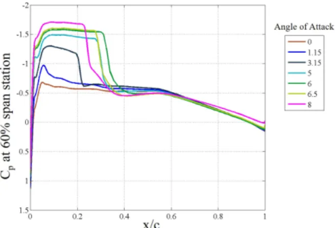
Mach numbers where the flutter dip occurs. It remains nearly stationary as the wing pitches or changes angle of attack. This characteristic is illustrated explicitly in Figure 13a, where slices of pressure coefficient on the wing upper surface at 60% span are shown for angles of attack between0◦ and8◦. These results were obtained from steady rigid analyses. Figure 13b shows experimental data sets that covers a smaller range of angle of attack at the same Mach number. This data shows a much different pressure profile and trends with increasing angle of attack. The upper surface shock location is shown to progress forward as the angle of attack increases, supporting the trends that were observed in the prior RANS simulations, but in contrast to those observed in the Euler simulations.
The lift curve slope, the pitching moment slope, the aerodynamic center location and the center of pressure were calculated from the Mach 0.87 rigid steady information. The lift curve slope and pitching moment curve slope were constant over the range of angle of attack examined, producing a constant value for the aerodynamic center at 40% chord, as shown in Figure 14. This is ahead of the elastic axis. The center of pressure is a function of angle of attack, and is aft of the elastic axis for the angles examined. This provides information to suggest that the transonic dip predicted by the Euler simulations is not simply associated with coincident location of the elastic axis with the location of either the center of pressure or the aerodynamic center.
(c) Lower Surface, Selected Pt #1. (d) Lower Surface, Selected Pt #2. Figure 12: Euler results, Mach 0.87,α= 5◦,q¯=25 psf.
(a) Euler results from rigid steady analyses. (b) Experimental data, upper surface. Figure 13: Pressure coefficents at 60% span, Mach 0.87.
5.2 RANS analyses
The previously reported RANS simulations were primarily at Mach 0.74 and 0.85, the primary analysis conditions for the AePW. Here, a more full exploration of the Mach number and angle-of-attack effects are pursued. An angle-angle-of-attack variation at Mach 0.85 is the first set of cases examined. The results from this initial set of cases show that the transonic dip is expected at a Mach number above 0.85 for 0◦ angle of attack and at a Mach number below 0.85 for α = 3.15◦ and 5◦. These results, discussed in detail below, agree with the general trends
Figure 14: Aerodynamic center migration vs. angle of attack, Euler results, Mach 0.87,α= 5◦,q¯=25 psf.
historically observed, including those shown in Figure 1.
This first set of cases uses the medium grid and the time step previously shown to produce temporally converged results (0.0002 seconds for each time step). The damping and frequency extracted from the time histories of the unstable mode, dominated by the pitch degree of free-dom, are shown in Figure 15 (forα = 0◦, 3.15◦ and5◦), comparing the data with Euler results at the same conditions. The Euler results have already been shown to be in the transonic dip for theα= 5◦ case. This is illustrated by the red squares, which show damping becoming negative at a low value of dynamic pressure. By contrast, theα = 5◦ RANS results are on the back side of the transonic dip, where flutter onset conditions rise dramatically to higher dynamic pressure (i.e., this condition is extremely stable). This is shown by the pink squares. The frequency of the mode remains close to the air-off pitch mode frequency (5.2 Hz) throughout the dynamic pressure range, and even increases at dynamic pressures above the flutter onset condition. This mechanism is dominated by pitching motion.
Decreasing the angle of attack to α = 3.15◦ further stabilizes the system in the RANS simu-lations, as shown by the light yellow triangles. The frequency behavior, however, resembles more of a coupled pitch-plunge frequency than that observed at α = 5◦. Although the flutter mechanism is likely different from that of theα= 5◦ case, the highly stable behavior indicates that forα= 3.15◦, any transonic dip likely occurs below the analyzed Mach number, 0.85. Decreasing the angle of attack further, to 0◦, changes the system behavior. This is shown by the blue circles on both the damping and frequency plots. The system frequency is lower for all dynamic pressures than at the higher angles of attack, indicating that this case involves more coupling between the higher frequency pitch mode and the lower frequency plunge mode. The damping plot shows that the system destabilizes atq¯=230 psf. This case is on the subsonic portion of the flutter boundary and any transonic dip forα= 0◦occurs at a higher Mach number. A significant number of additional RANS simulations were performed to define the flutter boundaries across the Mach number range. Results for four angles of attack are shown in Figure 16.
The flutter boundary forα= 0◦was not explored to a high enough Mach number to determine if there is a transonic dip associated with this angle of attack. Over the range examined, Mach 0.5-0.85, the flutter onset condition increases at Mach 0.82, but maintains the same flutter condition at Mach 0.85. Higher Mach number analyses are required to search for the flutter dip and the back side of the bucket for this case. As shown in the figure, there is little difference between
0.85, Medium grids. (Instability is indicated by negative values of damping.)
Figure 16: Flutter Buckets using URANS, Nominal parameters, across ranges of Mach and angle of attack.
results obtained using the medium grid and using the extra fine grid.
The flutter boundary for α = 3.15◦ shows a flat boundary until just above Mach 0.8. The predicted transonic bucket is very narrow in terms of Mach number and very shallow in terms of dynamic pressure drop. The bucket was only observable by performing simulations at very closely spaced Mach numbers (0.8, 0.805, 0.81, 0.8125, 0.815, 0.82). The total depth of the dip wasq¯=15 psf. Only results using the medium grid are currently available.
The flutter boundary forα = 4◦ using the coarse mesh is shown. This is the lowest examined angle of attack where a substantial flutter bucket is observed in the RANS simulations. Because a finer grid will likely change this boundary significantly, these results are not further discussed in this paper.
The flutter boundary for α = 5◦ shows a flutter bucket that is very deep and fairly wide. The α = 5◦flutter boundary is examined in more detail in Figure 17, where the results from multiple aerodynamic modeling methods are compared. The Euler flutter bucket, as discussed earlier, has a trough in the flutter boundary from Mach 0.86 to 0.88. The RANS results vary by grid refinement, by limiter presence and by turbulence model, although most of the results shown indicate that there is a dip in the flutter boundary near Mach 0.80. Experimental data and DDES results are also shown and also indicate a flutter dip near Mach 0.80.
While performing these analyses, additional cases were run and several cases were rerun to ex-amine the physics at play in the predictions. In reanalyzing, it was discovered that for numerous cases, including those at the bottom of the transonic dip, there is great sensitivity to very small
changes, including convergence level on the grid deformation scheme. At the bottom of the transonic dip, the use of a flux limiter was shown to influence the URANS simulation results, unlike those generated using Euler analysis. For the URANS simulations, the range in the flut-ter onset condition at Mach 0.80, α = 5◦ is shown overplotted with the flutter boundaries in Figure 18. The variations are large and demand further study.
Figure 17: Flutter Buckets,α= 5◦, Comparing all theories.
Figure 18: Range of flutter onset condition for URANS simulations overplotted with flutter boundaries; Mach 0.8 andα= 5◦.
6 CONCLUDING REMARKS
Analysis efforts for the BSCW have continued beyond the Aeroelastic Prediction Workshops. The configuration has proven immensely interesting and challenging. Different levels of aero-dynamic modeling have been utilized. The predictions of the transonic dips vary among the models. The RANS simulations predict a very deep flutter bucket for α = 5◦, to an unre-alistically low value of dynamic pressure, 0 psf, exclusive. There is great sensitivity of the damping observed in the simulations, which will require additional study. The depth of the RANS-predicted dip appears to be driven by separating and reattaching flow. The Euler sim-ulations at α = 5◦ also show a flutter bucket, at a higher Mach range, that dips to a dynamic pressure of 0 psf, exclusive. The predicted pressure distributions from Euler simulations don’t follow patterns shown in a limited set of available experimental data. The nature of the physics or mathematics that is responsible for the predictions of the transonic dip will require still more investigation. The sparseness of the experimental data has hindered evaluation of the suitability of the different aerodynamic models for predicting aeroelastic characteristics. A detailed data
Jacobson for sharing his insights into the CFD processes and results.
8 REFERENCES
[1] Edwards, J., Bennett, R., Whitlow, W. J., et al. (1983). Time-marching transonic flutter solutions including angle-of-attack effects. Journal of Aircraft, 20(11), 527–534.
[2] Dansberry, B., Durham, M., Bennett, R., et al. Experimental unsteady pressures at flutter on the supercritical wing benchmark model. AIAA paper 93-1592-CP. Presented at the AIAA Structural Dynamics and Materials Conference, April 1993.
[3] Piatak, D. and Cleckner, C. Oscillating turntable for the measurement of unsteady aero-dynamic phenomenon. Journal of Aircraft. Vol 40, No. 1, Jan-Feb 2003.
[4] Schuster, D. (2001). Aerodynamic measurements on a large splitter plate for the nasa langley transonic dynamics tunnel. NASA TM-2001-210828.
[5] Dansberry, B., Durham, M., Bennett, R., et al. (1993). Physical properties of the bench-mark models program supercritical wing. NASA TM-4457.
[6] Heeg, J., Wieseman, C., and Chwalowski, P. (2016). Data comparisons and summary of the second AIAA Aeroelastic Prediction Workshop. AIAA Paper 2016-3121. 34th AIAA Applied Aerodynamics Conference.
[7] Heeg, J. and Piatak, D. Experimental data from the benchmark supercriti-cal wing wind tunnel test on an oscillating turntable. AIAA-2013-1801. 54th AIAA/ASME/ASCE/AHS/ASC Structures, Structural Dynamics, and Materials Confer-ence, Boston, Massachusetts, Jan. 8-11, 2013.
[8] Heeg, J., Chwalowski, P., Schuster, D. M., et al. (2015). Plans and example results for the 2nd aiaa aeroelastic prediction workshop. AIAA Paper 2015-0437.
[9] Chwalowski, P., Heeg, J., and Biedron, R. (2017). Numerical investigations of the bench-mark supercritical wing in transonic flow. AIAA Paper 2017-0190.
[10] Biedron, R. T. et al. (2016). FUN3D Manual: 12.9. NASA, Hampton, VA. http://fun3d.larc.nasa.gov.
[12] Spalart, P. R. and Allmaras, S. R. A one-equation turbulence model for aerodynamic flows. La Recherche Aerospatiale, No. 1, 1994, pp 5–21.
[13] Roe, P. L. Approximate Riemann Solvers, Parameter Vectors, and Difference Schemes. Journal of Computational Physics. Vol. 43, No. 2, 1981.
[14] Vatsa, V. N., Carpenter, M. H., and Lockard, D. P. (2010). Re-evaluation of an optimized second order backward difference (bdf2opt) scheme for unsteady flow applications. AIAA Paper 2010-0122.
[15] Biedron, R. T. and Thomas, J. L. (2009). Recent enhancements to the fun3d flow solver for moving-mesh applications. AIAA Paper 2009-1360.
[16] Batina, J. T. (1987). Unsteady transonic flow calculations for realistic aircraft configura-tions. AIAA Paper 1987-0850.
[17] Bartels, R. E., Rumsey, C. L., and Biedron, R. T. (2006). Cfl3d version 6.4 - general usage and aeroelastic analysis. NASA TM 2006-214301.
[18] MSC Software, Santa Ana, CA (2008). MSC Nastran.
http://www.mscsoftware.com/products/msc nastran.cfm.
[19] Samareh, J. A. (2007). Discrete data transfer technique for fluid-structure interaction. AIAA Paper 2007-4309.
[20] Heeg, J. and Chwalowski, P. (2017). Investigating the transonic flutter boundary of the benchmark supercritical wing. AIAA Paper 2017-0191.
[21] Chwalowski, P. and Heeg, J. (2016). Fun3d analyses in support of the second aeroelastic prediction workshop. AIAA Paper 2016-3122.
![Figure 5: Flutter Boundary Results using FUN3D from AePW-2 [21].](https://thumb-us.123doks.com/thumbv2/123dok_us/1876821.2774015/7.892.298.593.102.365/figure-flutter-boundary-results-using-fun-d-aepw.webp)