University of Connecticut
OpenCommons@UConn
Doctoral Dissertations University of Connecticut Graduate School12-10-2015
Efficient Methods for Mining Association Rules
from Uncertain Data
Manal Hamed Alharbi [email protected]
Follow this and additional works at:https://opencommons.uconn.edu/dissertations Recommended Citation
Alharbi, Manal Hamed, "Efficient Methods for Mining Association Rules from Uncertain Data" (2015).Doctoral Dissertations. 952. https://opencommons.uconn.edu/dissertations/952
Efficient Methods for Mining Association Rules
from Uncertain Data
Manal Hamed Alharbi, PhD
University of Connecticut 2015
Association rules mining is a common data mining problem that explores the relationships among items based on their occurrences in transactions. Traditional approaches to mine frequent patterns may not be applicable for several real life applications. There are many domains such as social networks, sensor networks, protein-protein interaction analysis, and inaccurate surveys where the data are uncertain. As opposed to deterministic or certain data where the occurrences of items in transactions are definite, in an uncertain database, the occurrence of an item in a transaction is characterized as a discrete random variable and thus represented by a probability distribution. In this case the frequency of an item (or an itemset) is calculated as the expected number of occurrences of the item (itemset) in the transactions. In this research work, we present efficient computational algorithms for three important problems in data mining involving uncertain data. Specifically, we offer algorithms for weighted frequent pattern mining, disjunctive association rules mining, and causal rules mining, all from uncertain data. Even though
Manal Hamed Alharbi – University of Connecticut, 2015
algorithms can be found in the literature for these three versions of rules mining, we are the first ones to address these problems in the context of uncertain data.
I
Efficient Methods for Mining Association
Rules from Uncertain Data
Manal Hamed Alharbi
M.S., King Abdul-Aziz University, Saudi Arabia, 2008 B.A., King Abdul-Aziz University, Saudi Arabia, 1998
A Dissertation
Submitted in Partial Fulfillment of the Requirements for the Degree of
Doctor of Philosophy At the
University of Connecticut 2015
II
Copyright by
Manal Hamed Alharbi
III
APPROVAL PAGE
Doctor of Philosophy Dissertation
Efficient Methods for Mining Association Rules from
Uncertain Data
Presented by
Manal Hamed Alharbi, B.S., M.S.
Major Advisor _____________________________________________________ Sanguthevar Rajasekaran Associate Advisor__________________________________________________ Reda A. Ammar Associate Advisor__________________________________________________ Chun-Hsi Huang University of Connecticut 2015
IV
PREFACE
The Doctoral Dissertation “Efficient Methods for Mining Association Rules from Uncertain Data” is part of the research conducted at the Department of Computer Science and Engineering, University of Connecticut. The computing facilities at the department of Computer Science and Engineering were used for the purpose of this research. No human or animal subjects were involved in this research.
V
ACKNOWLEDGEMENTS
First and foremost, I must to praise and thank Allah (God) Almighty, who always helped and blessed me with his innumerable pure mercy in all my life.
My great praise, deepest appreciation and acknowledgment go to my major advisor Dr. Sanguthevar Rajasekaran for his incredible guidance and extraordinary intellectual support all the time of research and writing of this thesis. During my studies and research under his guidance I saw literally how being a smart successful teacher does not contradict with being a humble person. His patience, motivation and mentoring were the cornerstone to achieve my goal.
I would like to extend my sincere grateful, fulfillment, and gratitude to Dr. Reda Ammar who opened many doors for me as well as many of my colleagues and provided us the opportunity to be a part of this great research community. He was a father figure for all his students, and he spared no effort to help us in every aspect in this extraordinary journey in our lives. I would like to thank Dr. Chun-Hsi Huang for kindly agreeing to be on the panel of defense Committee members.
Thanks to the unknown soldier behind each success in my life, to my role model, to my father who was all his utterances, and deeds literally a reflection of the values and ideals that we read on books’ lines. Thanks to tribe of women, to my great teacher, to my mother who was a housewife and dedicated all her life to us. She had never eaten until
VI
we all finished, takes care of all her 14 kids, prays to Allah to continue his blessing on her house, and all other houses in every place in this world. I am extremely thankful to my family for their constant material and moral support, and for their unconditional love. I am grateful to have such loving sisters (Fawziah, Sameera, Huda, Eman, Nawal, Nisreen, Noha, Wafa, and Fatmah). My research would not have been possible without their help, and best wishes. Thanks to my dearest brothers (Yaser, Osama, Talal, and Mohammed) - you are always there for me no matter what I do or say. Special thanks to my wonderful Grandmother Nassra, to my precious brothers in law (Abdul Jabbar, Adel) who passed away during the completion of this work.
Thanks to my friends for their encouragement. I would like to especially thank my best friend Huda Alhazmi for knowing my weakness and showing me my strengths. She was always there, shared all my moments with me, and stood by me through the good and bad times.
Last but not least, words are not sufficient to appreciate the person who has a great impact on my life, for making my life much happier, for granting me the positive energy that keep pushing me to finish this research.
VII
Dedicated To
My father Hamed Eid Alharbi
Who taught me to smile in front of hardness, to value myselfwhenlightning strikes me, to fight for my rights, to chase my dreams, and to appreciate blessings of life.
To my father when he always told me…
VIII
Table of Contents
Chapter 1 ... 1
Introduction and Motivation ... 1
Chapter 2 ... 5
Association Rules Mining From Uncertain Data ... 5
2.1 Traditional Association Rules Mining ...5
2.1.1 Traditional Frequent Patterns Mining Algorithms ... 8
2.2 Association Rules Mining on Uncertain Data ... 18
2.2.1 Frequent patterns Algorithms for Uncertain Data ... 20
Chapter 3 ... 23
Frequent Itemsets Mining From Weighted Uncertain Data ... 23
3.1 Introduction ... 23
3.2 Weighted frequent pattern mining algorithms on certain database ... 25
3.3 Proposed Algorithms of Weighted frequent pattern mining algorithms on uncertain data ... 28
3.3.1 Horizontal Weighted Uncertain Apriori (𝑯𝑾𝑼𝑨𝑷𝑹𝑰𝑶𝑹𝑰) ... 31
3.3.2 Vertical Weighted Uncertain Frequent itemset Mining Algorithm 𝑽𝑾𝑼𝑭𝑰𝑴... 33
3.4 Complexity Analysis: ... 35
3.4.1 Time Complexity Analysis for HWUAPRIORI: ... 35
3.4.2 Time Complexity Analysis for VWUFIM: ... 36
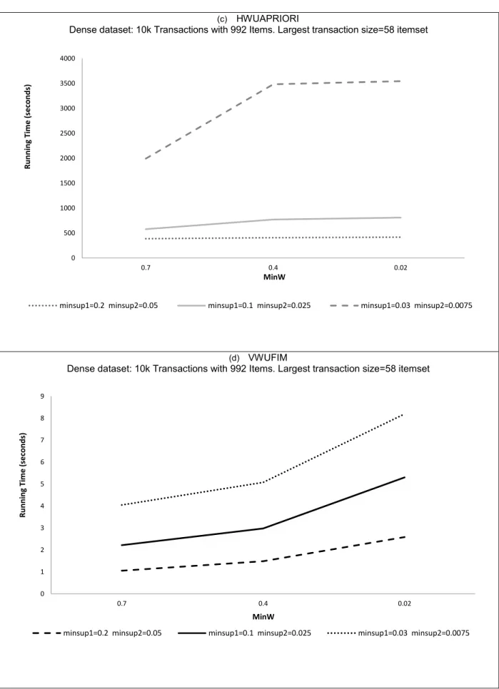
3.5 Experimental Results ... 36
3.6 Conclusion ... 37
Chapter 4 ... 42
Disjunctive Rules Mining From Uncertain Data... 42
4.1 introduction ... 42
4.1.1 Motivating Applications ... 44
4.2 Disjunctive Rules Miner from Uncertain Databases (DRMUD) ... 45
4.2.1 DRMUD Algorithm ... 48
4.3 Complexity Analysis ... 50
4.4 Experimental Results ... 50
4.4.1 Horizontal vs. Vertical DRMUD algorithm ... 55
4.5 Conclusions ... 62
IX
Causal Rules Mining From Uncertain Data ... 63
5.1 Introduction ... 63
5.1.1 Causal Discovery ... 64
5.2 Definitions ... 66
5.2.1 Correlations vs. Traditional Support-Confidence Frame-work ... 67
5.2.2 Rule discovery using partial association test ... 70
5.3 Proposed Methods: ... 72
5.3.1 Disjunctive Association Rules Mining from Uncertain Data... 72
5.3.1.1 Disjunctive Combined Causal Rules from Uncertain Data Algorithm- (DCCRUD) ... 73
5.3.2 Conjunctive Association Rules Mining from Uncertain Data ... 76
5.3.2.1 Conjunctive Combined Causal Rules from Uncertain Data Algorithm- (CCCRUD) ... 76
5.4 Complexity Analysis ... 79
5.4.1 DCCRUD Complexity Analysis ... 80
5.4.2 CCCRUD Complexity Analysis ... 83
5.5 EXPERIMENTAL RESULTS ... 85
5.5.1 CCRCD algorithm V.s. CR-PA algorithm ... 85
5.5.2 Experimental Results for DCCUCM Algorithm ... 87
5.5.3 Experimental Results for CCCUCM Algorithm ... 90
5.6 Conclusions ... 92
Chapter 6 ... 94
Concluding Remarks and Future Directions ... 94
X
LIST OF FIGURES
Fig. 3.1. Performance of HWUAPRIORI and VWUFIMover algorithms ...39
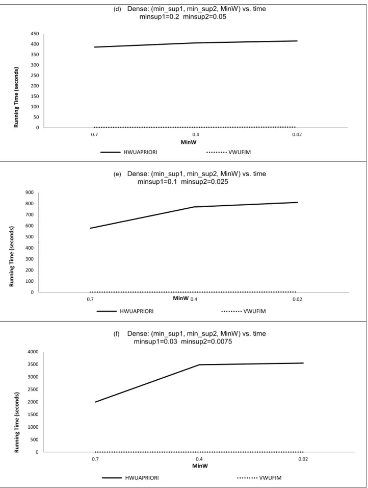
Fig. 3.2. Comparisons between 𝐻𝑊𝑈𝐴𝑃𝑅𝐼𝑂𝑅𝐼 and 𝑉𝑊𝑈𝐹𝐼𝑀 algorithms ...41
Fig. 4.1. Performance of Horizontal DRMUM algorithm ...54
Fig. 4.3. Comparisons between Horizontal and Vertical for DRMUD algorithms ...61
Fig. 5.1. Performance of DCCRUD algorithm ...88
Fig.5.2. Scale-up of attributes ...89
Fig. 5.3. Run time Vs. 𝑚𝑖𝑛𝑖𝑚𝑢𝑚 𝑠𝑢𝑝𝑝𝑜𝑟𝑡 ...89
Fig. 5.4. Performance of 𝐶𝐶𝐶𝑅𝑈𝐷 algorithm ...91
Fig. 5.5. Scale-up of attributes ...92
I
LIST OF TABLES
Table 2.1: Transactional Database ... 6
Table 2.2: Support for Itemsets for example 2.3 ... 8
Table 2.3: Confidence of large itemset for example 2.3 ... 9
Table 2.4: Summary of Sequential Algorithms...10
Continuation of Table 2.4: Summary of Sequential Algorithms ...11
Table 2.6: Transactional Database for example 2.4 ...13
Table 2.7: Support for the first and second Candidates for example 2.4 ...13
Table 2.8: Data parallelism paradigm ...13
Table 2.9: Task parallelism paradigm ...14
Table 2.10: Summary of Parallel Algorithms under 𝑡ℎ𝑒 𝐷𝑃 Paradigm ...14
Table 2.11: Summary of Parallel Algorithms under 𝑇𝑃 Paradigm ...15
Table 2.12: Horizontal Layout ...16
Table 2.13: Vertical Layout...16
Table 2.14: The four cases of itemsets on an updated database ...17
Table 2.15: The nine cases of itemsets in an updated database ...18
Table 2.16: An uncertain database...20
Table 3.1: Certain data for example 3.1 ...25
Table 3.2: Items’ weights for example 3.1 ...25
Table 3.3: Weighed transactional certain data for example 3.2 ...26
Table 3.4: uncertain transaction database for example 3.3 ...29
Table 3.5: Item’s weight for example 3.3 ...29
Table 4.1 uncertain transaction database ...47
Table 4.2: Result of horizontal 𝐷𝑅𝑀𝑈𝐷 under Dense dataset, 40K trans. with 994 Items ...51
Table 4.3: Result of horizontal 𝐷𝑅𝑀𝑈𝐷 under Dense dataset 20K trans. with 994 items ...52
Table 4.4: Result of horizontal 𝐷𝑅𝑀𝑈𝐷 under synthData dataset, 10K Trans. with 20 Items ...53
Table 4.5: Result of horizontal 𝐷𝑅𝑀𝑈𝐷 under Gazelle sparse dataset, 59602 Trans. with 994 Items ...54
Table 4.6: Result of vertical 𝐷𝑅𝑀𝑈𝐷under Dense dataset, 40K trans. with 994 Items ...56
II
Table 4.8: Result of vertical 𝐷𝑅𝑀𝑈𝐷under synthData Dense dataset, 10K Trans. with 20 Items
...58
Table 4.9: Result of vertical 𝐷𝑅𝑀𝑈𝐷under Gazelle sparse dataset, 59602 Trans. with 994 Items ...59
Table 5.1: 𝟐 × 𝟐 Contingency Table ...68
Table 5.2: 𝟐 × 𝟐 Combined Contingency Table ...69
Table 5.3: Contingency Table for Partial Association Test ...71
Table 5.4: Dataset 1- Causal Rules under p=0.05, min. support=0.05 ...86
Table 5.5: Dataset 2 - Causal Rules under p=0.05, min. support=0.01 ...86
Table 5.6: Dataset 2- Causal Rules under p=0.1, min. support=0.01 ...86
Table 5.7: Dataset 2- Disjunctive single and combined Causal Rules DCCRUD ...88
1
Chapter 1
Introduction and Motivation
Frequent pattern mining is a well-studied problem that aims to discover the relationships among items based on their occurrences in transactions. Due to the growth of applications that involve uncertain data, traditional approaches to mine frequent patterns may not be applicable for several real life applications. In recent years, quality research has been conducted to associate the occurrences of items in uncertain databases for applications like social networks, sensor networks, protein-protein interaction analysis and inaccurate surveys. Uncertainty could also arise from masking of data for privacy concerns. Unlike certain data where the occurrences of items in transactions are definite, in an uncertain database, we are not sure about the items that occur in any transaction. Instead, we only know a probability for each possible item that this item belongs to a given transaction. In this thesis, we focus on three important problems in data mining involving uncertain data. Specifically, we propose two algorithms for weighted frequent patterns mining, a disjunctive association rules mining algorithm, and two algorithms for discovering both conjunctive and disjunctive causal rules mining, all from uncertain data. In spite of the fact that some algorithms have been introduced in
2
the literature for these three versions of rules mining, we believe that this is the first work that addresses these problems in the context of uncertain data.
Weighted frequent pattern mining is the problem that introduces the importance of an item as a significant factor besides its frequency. Unlike the typical frequent pattern mining methods that treat items as equally important, here we consider the case when each item has a different level of importance. The importance of weight-based pattern mining approach can be felt in many domains such as, biomedical data analysis where the causes of most diseases are not only one gene but a combination of genes; web traversal pattern mining where the impact of each web page is different; and so on. Thus, many algorithms have been proposed for weighting items based on their significance. To the best of our knowledge, no algorithms have been proposed in the literature for mining from uncertain weighted data. In this thesis we investigate the problem of mining from uncertain weighted data and present theoretical and experimental results for the proposed methods.
Disjunctive association rules mining is the problem when the antecedent and the consequent are sets of disjunctions (of items). A typical algorithm for association rules mining can be thought of as a conjunctive rule. There are many applications where rules with the antecedent as well as the consequent consisting of disjunctions of item sets might be relevant. The problem of generating disjunctive rules has been studied well. All the existing works on disjunctive rules thus far have been carried out to find disjunctive rules on databases without uncertainty. No work has been done on identifying disjunctive rules from uncertain data. The problem of disjunctive rules mining from uncertain data has numerous applications especially in biology, medicine, and bioinformatics. One of the
3
challenges in generating disjunctive rules lies in the need to explore a large collection of possible antecedents and consequents. Existing algorithms have large run times. In this research work, we propose an efficient algorithm for mining disjunctive rules from uncertain data.
Causal rules mining is the problem that mainly aims to discover profound relationships such as a change of antecedent is the cause for a change in the consequent. Traditional association rules mining algorithms identify the relationships among variables. By using support –confidence framework, we can show whether the antecedent and the consequent of a rule are related or not in general. However, associations do not necessarily signify causation. There are many cases where if the causes are predicted, we can easily avoid the consequences. The importance of causal relationships from uncertain data can be felt in many areas, such as economics, physical, behavioral, medical, biological, and social sciences. Statisticians have conducted many previous works in the direction of identifying causal rules. Also, partial association tests have been integrated along with association rule mining to minimize the exponential runtimes with the traditional statistical approaches of discovering Causal relationships. In this thesis we propose novel algorithms for finding both conjunctive and disjunctive Causal rules from uncertain transactional databases.
The rest of the dissertation is divided into five sections. In chapter 2, we present a summary on association rules mining algorithms, and discuss its most important algorithms for both certain and uncertain data. Also, we highlight the relative advantages and shortcomings of the different existing algorithms. In Chapter 3, we propose new algorithms for frequent itemsets mining on weighted uncertain data. In Chapter 4, we
4
present a novel algorithm for disjunctive rules mining from uncertain data. In Chapter 5, we propose new algorithms for both conjunctive and disjunctive Causal rules mining from uncertain data. Finally, we present our conclusions and describe future work in Chapter 6.
5
Chapter 2
Association Rules Mining From Uncertain Data
2.1 Traditional Association Rules Mining
Association rules mining is an important and well-researched problem in data mining which aims to find hidden relationships among items in large databases. Association rules mining algorithms have proven to be quite useful in many diverse fields including Web usage mining, intrusion detection, bioinformatics, etc. One of the first algorithms proposed for this problem was by Agrawal, et al. [1]. They introduced the idea for generating association rules from large scale transaction data in the context of the market basket problem. For example, a rule like {milk} ⇒ {diaper} from a supermarket data indicates that when a person buys milk then (s)he is also likely to buy diaper. Knowing such information can be very useful for making proper decisions that increase the efficiency and reduce the cost associated with marketing activities such as product placements and promotional pricing [2].
Definition 2.1: A typical transactional dataset 𝑇 consists of set of transactions where each transaction 𝑡 comprises of a number of unordered items. The problem of
6
association rules mining can be stated as follows [1]: let the set of all possible items be
𝐼 = {𝑖1, 𝑖2, ⋯ , 𝑖𝑚}. Each transaction 𝑡 can be thought of as a subset of 𝐼. A subset of items is also known as an itemset. A 𝑘 − 𝑖𝑡𝑒𝑚𝑠𝑒𝑡 is an itemset with 𝑘 items. An association rule is nothing but an implication of the form 𝑋 ⇒ 𝑌, where 𝑋 ⊂ 𝐼, 𝑌 ⊂ 𝐼, and 𝑋 ⋂ 𝑌 = ∅. Here
𝑋 and 𝑌 are defined as the antecedent and consequent of the rule, respectively.
Table 2.1shows an example. Table 2.1 in the left shows the itemset in binary format, where 1 signifies presence, and 0 signifies absence of any item in a transaction. Table 2.1 on the right shows a different representation of the itemsets in the transactions.
Table 2.1: Transactional Database Transaction ID milk egg diaper beer
1 1 1 1 0 2 1 0 1 0 3 0 1 0 1 4 1 1 0 1 5 0 1 1 1 ≡ Transaction ID Items
𝑇1 milk, egg, diaper
𝑇2 milk, diaper
𝑇3 egg, beer
𝑇4 milk, egg, beer
𝑇5 milk, egg, beer
Support and confidence of a rule are two measures that signify the importance of the rule.
Definition 2.2: Support of a rule 𝑋 ⇒ 𝑌 is defined as the fraction of transactions that contain both 𝑋 and 𝑌. support(𝑋 ∪ 𝑌) =𝑡𝑜𝑡𝑎𝑙 𝑛𝑢𝑚𝑏𝑒𝑟 𝑜𝑓 𝑟𝑒𝑐𝑜𝑟𝑑𝑠 𝑖𝑛 𝑡ℎ𝑒 𝑑𝑎𝑡𝑎𝑏𝑎𝑠𝑒𝑛𝑢𝑚𝑏𝑒𝑟 𝑜𝑓 𝑟𝑒𝑐𝑜𝑟𝑑𝑠 𝑡ℎ𝑎𝑡 𝑐𝑜𝑛𝑡𝑎𝑖𝑛 𝑋 ∪ 𝑌 .
Example 2.1: the support of the rule {milk} ⇒ {diaper} = 25= 0.4 = 40%.
Definition 2.3: Confidence of a rule is defined as the number of transactions in which both 𝑋 and 𝑌 occur divided by the number of transactions in which 𝑋 occurs.
𝐶𝑜𝑛𝑓𝑖𝑑𝑒𝑛𝑐𝑒(𝑋 ⇒ 𝑌) =sup( 𝑋 ∪ 𝑌)sup(𝑋) .
7
From among all such possible implications, only some of them could be of interest to us. Rules of importance are normally characterized with two parameters; 𝑚𝑖𝑛𝑠𝑢𝑝, and
𝑚𝑖𝑛𝑐𝑜𝑛𝑓, where the support of the rule implies that support(𝑋 ∪ 𝑌) has to be at least
𝑚𝑖𝑛𝑠𝑢𝑝 and confidence of the rule stipulates that 𝑐𝑜𝑛𝑓𝑖𝑑𝑒𝑛𝑐𝑒(𝑋 ⇒ 𝑌) has to be at least
𝑚𝑖𝑛𝑐𝑜𝑛𝑓. Any itemset is said to be frequent if its support is at least 𝑚𝑖𝑛𝑠𝑢𝑝. Both 𝑚𝑖𝑛𝑠𝑢𝑝
and 𝑚𝑖𝑛𝑐𝑜𝑛𝑓 thresholds are user-defined values ∈ [0,1]
An important question is: How can we determine the best value for 𝑚𝑖𝑛𝑠𝑢𝑝 and
minconf thresholds? In fact, there is no straightforward answer for this question and
generally speaking, 𝑚𝑖𝑛𝑠𝑢𝑝 threshold is usually chosen through trial and error. Setting
𝑚𝑖𝑛𝑠𝑢𝑝 with a low value may lead to the generation of too many uninteresting frequent itemsets, and an increase in the time complexity. However, setting 𝑚𝑖𝑛𝑠𝑢𝑝 with a high value will improve the run time but may lead to the generation of no (or a very low number of) frequent itemsets.
Philippe in his PhD thesis [3, 4] suggested a mathematical function that allows one to modify the 𝑚𝑖𝑛𝑠𝑢𝑝 threshold dynamically based on the database size. He used this equation: = (𝑒(−𝑎𝑁−𝑏))+ 𝑐 , where 𝑎, 𝑏, 𝑐 are constants, and 𝑁 represents the number of
transactions.
In this thesis, we used the trial and error method. We set the 𝑚𝑖𝑛𝑠𝑢𝑝 parameter with a low value and then we gradually increase it until we extract a sufficient number of interesting patterns within a reasonable amount of time. For the 𝑚𝑖𝑛𝑐𝑜𝑛𝑓, we need to have a value of at least 50% for a rule to be interesting.
8
2.1.1 Traditional Frequent Patterns Mining Algorithms
A typical algorithm for association rules mining consists of two phases. In the first phase all the frequent itemsets are identified by searching through all possible Itemsets. Thus, it requires 2𝑛−1 time where 𝑛 is the number of items in 𝐼. In the second phase, the
frequent itemsets are used to generate association rules. The second phase is relatively simpler compared to the first phase and hence researchers mostly tackle the problem of identifying frequent itemsets. One of the most useful strategies that can be used to reduce the number of generated candidates is the 𝑑𝑜𝑤𝑛𝑤𝑎𝑟𝑑 𝑐𝑙𝑜𝑠𝑢𝑟𝑒 𝑝𝑟𝑜𝑝𝑒𝑟𝑡𝑦 [1].
𝐷𝑜𝑤𝑛𝑤𝑎𝑟𝑑 𝑐𝑙𝑜𝑠𝑢𝑟𝑒 𝑝𝑟𝑜𝑝𝑒𝑟𝑡𝑦 states that any subset of a frequent itemset is also frequent which implies that any superset of an infrequent itemset is also infrequent.
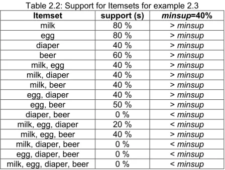
Example 2.3: Table 2.2, and Table 2.3 illustrate the strategy of finding association rules from large Itemsets, assume 𝑚𝑖𝑛𝑠𝑢𝑝 = 40%, and 𝑚𝑖𝑛𝑐𝑜𝑛𝑓 = 60%. For the transactional database in table 2.1, table 2.2 shows the frequent itemsets, and table 2.3 shows the association rules.
Table 2.2: Support for Itemsets for example 2.3
Itemset support (s) minsup=40%
milk 80 % > minsup
egg 80 % > minsup
diaper 40 % > minsup
beer 60 % > minsup
milk, egg 40 % > minsup
milk, diaper 40 % > minsup
milk, beer 40 % > minsup
egg, diaper 40 % > minsup
egg, beer 50 % > minsup
diaper, beer 0 % < minsup
milk, egg, diaper 20 % < minsup
milk, egg, beer 40 % > minsup
milk, diaper, beer 0 % < minsup
egg, diaper, beer 0 % < minsup
9
Table 2.3: Confidence of large itemset for example 2.3
Rule Confidence (𝜶) Rules Hold
milk ⇒ egg = 0.4/0.8 = 50 % No
milk ⇒ diaper = 0.4/0.8 = 50 % No
milk ⇒ beer = 0.4/0.8 = 50 % No
egg ⇒ diaper = 0.4/0.8 = 50 % No
egg ⇒ beer = 0.5/0.8 = 63 % Yes
milk, egg ⇒ beer = 0.4/0.4 = 100 % Yes
In general, rules mining algorithms are classified under two different approaches, namely, the level-wise approach [1, 2, 7-10] and the FP-tree growth approach [11, 12]. The well-known 𝐴𝑝𝑟𝑖𝑜𝑟𝑖 algorithm uses the level-wise approach [1]. It scans the database multiple times to generate all frequent Itemsets. It first generates candidate Itemsets of size one, and calculates the support count for each single item. Then, It applies the
𝑑𝑜𝑤𝑛𝑤𝑎𝑟𝑑 𝑐𝑙𝑜𝑠𝑢𝑟𝑒 𝑝𝑟𝑜𝑝𝑒𝑟𝑡𝑦 to delete all infrequent itemsets. In the second round, Apriori generates candidate Itemsets of size two. It repeats the process until there is no candidate left. FP-tree growth improves the Apriori algorithm by reducing the number of database scans employed by Apriori [11]. FP-tree growth generates the frequent Itemsets with only two rounds over the database and without any candidate generation process. It first builds a data structure called FP-tree with two scans through the data. Then, it traverses through the tree to generate the frequent itemsets. FP-tree growth approach outperforms level-wise approach by only needing two rounds to scan the database.
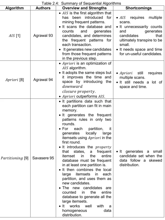
Numerous algorithms are available in the literature for association rules mining that are either sequential [1, 7-12] or parallel [13-19]. In general, sequential algorithms are proposed based on the assumption that Itemsets are stored such that itemsets can be easily counted based on their lexicographical order [5]. Some key sequential algorithms are summarized in table 2.4. Other algorithms are extended versions of these algorithms.
10
Table 2.4: Summary of Sequential Algorithms
Algorithm Authors Overview and Strengths Shortcomings
𝐴𝐼𝑆 [1] Agrawal 93
𝐴𝐼𝑆 is the first algorithm that
has been introduced for mining frequent patterns.
It scans the database and
counts and generates
candidates, and determines the frequent patterns for each transaction.
It generates new candidates
from those frequent patterns in the previous step.
𝐴𝐼𝑆 requires multiple scans. It unnecessarily counts and generates candidates that ultimately transpire to be small.
It needs space and time
for un-useful candidates.
𝐴𝑝𝑟𝑖𝑜𝑟𝑖 [8] Agrawal 94
𝐴𝑝𝑟𝑖𝑜𝑟𝑖 is an optimization of
𝐴𝐼𝑆 algorithm.
It adopts the same steps but
it improves the time and space by introducing the 𝑑𝑜𝑤𝑛𝑤𝑎𝑟𝑑
𝑐𝑙𝑜𝑠𝑢𝑟𝑒 𝑝𝑟𝑜𝑝𝑒𝑟𝑡𝑦.
𝐴𝑝𝑟𝑖𝑜𝑟𝑖 outperforms 𝐴𝐼𝑆.
𝐴𝑝𝑟𝑖𝑜𝑟𝑖 still requires multiple scans.
It still needs a lot of
space and time.
𝑃𝑎𝑟𝑡𝑖𝑡𝑖𝑜𝑛𝑖𝑛𝑔 [9] Savasere 95
It partitions data such that
each partition can fit in main memory.
It generates the frequent
patterns rules in only two rounds.
For each partition, it
generates locally large
itemsets using 𝐴𝑝𝑟𝑖𝑜𝑟𝑖 in the
first round.
It introduces the 𝑝𝑟𝑜𝑝𝑒𝑟𝑡𝑦
that states, a frequent
itemset in the entire
database must be frequent in at least one partition is.
It then combines the local
large itemsets in each partition, and uses them as new candidates.
The new candidates are
counted in the entire
database to generate all the large itemsets.
It works well with a
homogeneous data
distribution.
It generates a small
candidate set when the data follow a skewed distribution.
11
Continuation of Table 2.4: Summary of Sequential Algorithms
Algorithm Authors Overview and Strengths Shortcomings
𝑆𝑎𝑚𝑝𝑙𝑖𝑛𝑔 [10] Toivonen 96
It generates the frequent
patterns rules in one round in the best case, and only two rounds in the worst case.
It first chooses a random
sample that can fit in the main memory.
It generates the frequent
patterns using 𝐴𝑝𝑟𝑖𝑜𝑟𝑖 from
this random sample instead of the entire database.
It introduces
𝑁𝑒𝑔𝑎𝑡𝑖𝑣𝑒 𝐵𝑜𝑟𝑑𝑒𝑟 to generate more possible candidates, and use the rest of the database to verify the support of the candidates. 𝑁𝑒𝑔𝑎𝑡𝑖𝑣𝑒 𝐵𝑜𝑟𝑑𝑒𝑟 is a set
that contains closest
itemsets that could be frequent, and are not in the given frequent itemsets in the sample but have subsets of the frequent itemsets in the sample..
Second scan to the
database may be
needed to generate
another random sample In case of failure to find at least one frequent itemset in the negative border.
Thus, a large number of
candidates might be found.
𝐹𝑃 − 𝑇𝑟𝑒𝑒 [11] Han 2000
𝐹𝑃 − 𝑇𝑟𝑒𝑒 is designed to handle the disadvantages that are associated with
𝐴𝑝𝑟𝑖𝑜𝑟𝑖 algorithm such as the complexity and the
multiple scans of the
database.
It is faster than the 𝐴𝑝𝑟𝑖𝑜𝑟𝑖
algorithm since it generates the frequent Itemsets in two rounds and does not require any candidate generation approach.
Unlike 𝐴𝑝𝑟𝑖𝑜𝑟𝑖, it uses a
compact data structure in order to avoid multiple
scanning to generate
candidates.
𝐹𝑃 − 𝑇𝑟𝑒𝑒 consumes space.
It is not suitable when the
database is updated by adding new records or deleting existing ones.
12
On the other hand, the aim of parallel algorithms is to reduce the sequential algorithms’ complexity by parallelizing the process of identifying large itemsets. Dunham et al. [5] classified most parallel or distributed association rules mining algorithms under two paradigms: data parallelism (𝐷𝑃) algorithms aim to parallelize data, and task parallelism (𝑇𝑃) algorithms aim to parallelize the candidates.
Data Parallelism Algorithms: Let 𝐶 represent the set of candidates, and 𝑃
represent the set of processors {𝑃1, 𝑃2, … … . , 𝑃𝑛}, such that 𝐶 is duplicated on all processors. Let 𝐷 represent the database {𝑑1, 𝑑2, … … . , 𝑑𝑚} that is distributed over the processors. Let the set of support counts {𝑠1, 𝑠2, … … . , 𝑠𝑐} represent the local support
counts of all the candidates that are computed by the processors. Each processor is responsible for its own database. Let Global support counts represent the total support counts of the candidates in the entire database. The Global support counts of the candidates are computed in parallel for all the processors. This process is called Global
Reduction, and can be done by swapping the local support counts. Finally, each
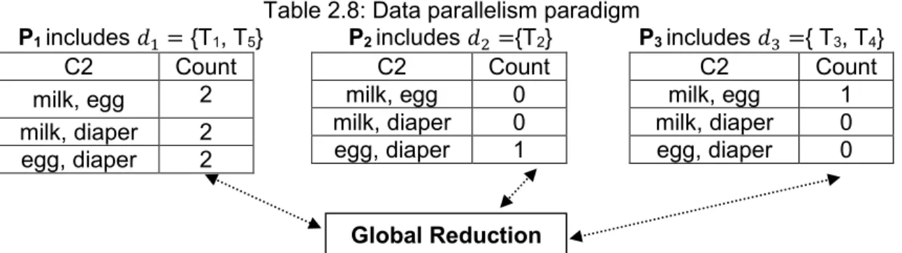
processor independently computes the large Itemsets. Example 2.4 illustrates the concept of this task.
Example 2.4: Using the data in Table 2.6, the five transactions are partitioned across the three processors (𝑃1, 𝑃2, 𝑃3) as shown in table 2.8. Let 𝑃1 = {𝑇1, 𝑇5}, 𝑃2 = {𝑇2}, and 𝑃3 = {𝑇3, 𝑇4}. The candidate Itemsets in the second scan are duplicated on each processor.
13
Table 2.6: Transactional Database for example 2.4
Transaction ID Items
𝑇1 milk, egg, diaper
𝑇2 egg, diaper, beer
𝑇3 egg
𝑇4 milk, egg
𝑇5 milk, egg, diaper
Table 2.7: Support for the first and second Candidates for example 2.4
Itemset support (s) minsup=40%
milk 60 % > minsup
egg 100 % > minsup
diaper 60 % > minsup
beer 20 % < minsup
milk, egg 60 % > minsup
milk, diaper 40 % > minsup
egg, diaper 40 % > minsup
Table 2.8: Data parallelism paradigm
P1 includes 𝑑1= {T1, T5} P2 includes 𝑑2={T2} P3 includes 𝑑3={ T3, T4}
C2 Count milk, egg 2 milk, diaper 2 egg, diaper 2 C2 Count milk, egg 0 milk, diaper 0 egg, diaper 1 C2 Count milk, egg 1 milk, diaper 0 egg, diaper 0
Task Parallelism Algorithms: Let 𝐶 represent the set of candidates, let 𝑃
represent the set of processors {𝑃1, 𝑃2, … … . , 𝑃𝑛}, and let 𝐷 represent the database
{𝑑1, 𝑑2, … … . , 𝑑𝑚} such that 𝐶 is partitioned into {𝑐1, 𝑐2, … … . , 𝑐𝑘} and distributed across the
processors {𝑃1, 𝑃2, … … . , 𝑃𝑛} as is the database {𝑑1, 𝑑2, … … . , 𝑑𝑚}. In this paradigm, the
Global support counts of the candidates are computed by each processor independently.
This task can be done in only two rounds; firstly, each processor broadcasts its own candidates to the rest of the processors to calculate the large Itemsets. Then, after each processor calculates its own large Itemsets, they send their own large Itemsets to the rest
14
of the processors in order to compute the new candidates. Example 2.5 illustrates the concept of this task.
Example 2.5: Using the data in Table 2.7, the five transactions are partitioned across the three processors (𝑃1, 𝑃2, 𝑃3) as shown in table 2.9. Let us partition the candidate Itemsets across the processors with each processor having one candidate Itemset.
Table 2.9: Task parallelism paradigm
P1 includes = { milk, egg } P2 includes ={milk, diaper} P3 includes ={egg, diaper}
C2 Count milk, egg 3 C2 Count milk, diaper 2 C2 Count egg, diaper 3
Count Distribution (CD) algorithm [13] uses the data parallelism (𝐷𝑃) paradigm, and follows the same steps as the algorithm above. Most of the parallel algorithms fall under 𝐷𝑃 and are extended versions of 𝑡ℎ𝑒 CD algorithm. They are summarized in table 2.10.
Table 2.10: Summary of Parallel Algorithms under 𝑡ℎ𝑒 𝐷𝑃 Paradigm
Algorithm Authors Overview and Strengths Shortcomings
𝑃𝑎𝑟𝑎𝑙𝑙𝑒𝑙 𝐷𝑎𝑡𝑎 𝑀𝑖𝑛𝑖𝑛𝑔 PDM Algorithm
[14]
Park 95a
PDM utilizes memory better than
CD as direct hashing technique is
added to prune some candidates in the second round.
PDM needs to
exchange not only the local counts of the candidate k-itemsets, but also the local counts in the hash table for k+1-itemsets.
𝐶𝑜𝑚𝑚𝑜𝑛 𝐶𝑎𝑛𝑑𝑖𝑑𝑎𝑡𝑒 𝑃𝑎𝑟𝑡𝑖𝑡𝑖𝑜𝑛𝑒𝑑 𝐷𝑎𝑡𝑎𝑏𝑎𝑠𝑒 𝐶𝐶𝑃𝐷 𝐴𝑙𝑔𝑜𝑟𝑖𝑡ℎ𝑚 [15] Zaki 96
𝐶𝐶𝑃𝐷 generates and counts candidates in a shared-memory since it was proposed on a shared-memory system.
It uses the common prefixes (ex.
the first item) to group large itemsets into equivalence classes, and then generates candidates from those classes.
To improve counting the
candidates for each transaction, CCPD as well employs a short-circuited subset checking method.
The common prefixes
technique to group large itemsets helps
in reducing the
candidates
generating time.
However it does not reduce the number of generated
candidates.
15
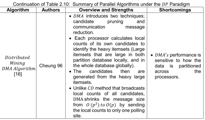
Continuation of Table 2.10: Summary of Parallel Algorithms under the 𝐷𝑃 Paradigm
Algorithm Authors Overview and Strengths Shortcomings
𝐷𝑖𝑠𝑡𝑟𝑖𝑏𝑢𝑡𝑒𝑑 𝑀𝑖𝑛𝑖𝑛𝑔 𝐷𝑀𝐴 𝐴𝑙𝑔𝑜𝑟𝑖𝑡ℎ𝑚
[16]
Cheung 96
𝐷𝑀𝐴 introduces two techniques;
candidate pruning and
communication message
reduction.
Each processor calculates local
counts of its own candidates to identify the heavy itemsets (Large itemsets that are large in both partition database locally, and in the whole database globally).
The candidates then are
generated from the heavy large itemsets.
Unlike 𝐶𝐷 method that broadcasts
local counts of all candidates,
DMA shrinks the message size
from 𝑂 (𝑝2) 𝑡𝑜 𝑂(𝑝) by sending
the local counts to only one polling site.
𝐷𝑀𝐴′𝑠 performance is sensitive to how the data is partitioned
across the
processors.
𝐷𝑎𝑡𝑎 𝐷𝑖𝑠𝑡𝑟𝑖𝑏𝑢𝑡𝑖𝑜𝑛 (𝐷𝐷) algorithm [13] is follows the data parallelism (𝑇𝑃)
paradigm, and follows the same steps of task parallelism algorithm above. Most of the parallel algorithms under 𝑇𝑃 are extended versions of the 𝐷𝐷 algorithm, and they are summarized in table 2.11.
Table 2.11: Summary of Parallel Algorithms under 𝑇𝑃 Paradigm
Algorithm Authors Overview and Strengths Shortcomings
𝐻𝑎𝑠ℎ 𝑏𝑎𝑠𝑒𝑑 𝑃𝑎𝑟𝑎𝑙𝑙𝑒𝑙 𝐴𝑠𝑠𝑜𝑐𝑖𝑎𝑡𝑖𝑜𝑛 𝑚𝑖𝑛𝑖𝑛𝑔 𝑜𝑓 𝐴𝑠𝑠𝑜𝑐𝑖𝑎𝑡𝑖𝑜𝑛 𝑟𝑢𝑙𝑒𝑠 𝐻𝑃𝐴 𝐴𝑙𝑔𝑜𝑟𝑖𝑡ℎ𝑚 [17] Shintani 96
𝐻𝑃𝐴 uses a hash function to
distribute, generate and count
the candidates through
processors.
Instead of allocating the
database partitions in the
processors, 𝐻𝑃𝐴 only sends
subset itemsets of the
transactions.
It also uses skew handling
technique, in order to achieve a load-balance for the candidates in each processor.
It involves the
maintenance of a Hash tree.
16
Continuation of Table 2.11: Summary of Parallel Algorithms under 𝑇𝑃 Paradigm
Algorithm Authors Overview and Strengths Shortcomings
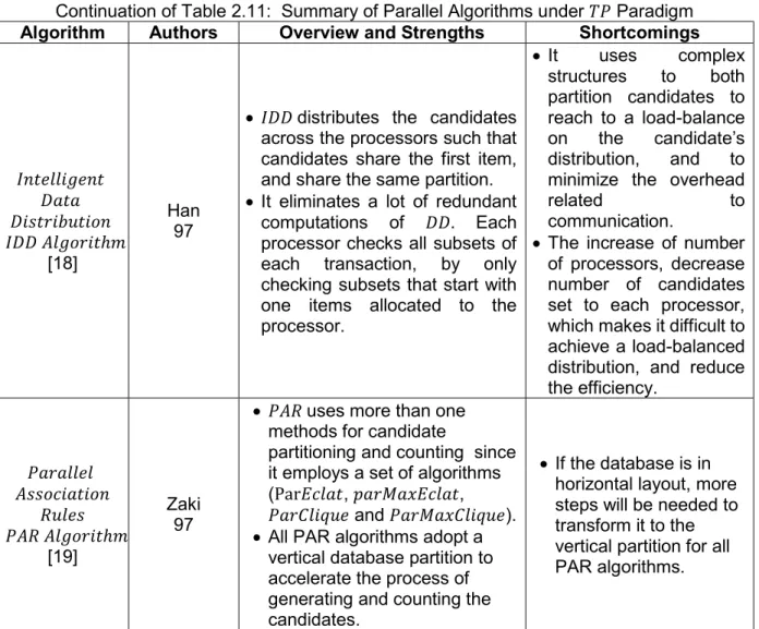
𝐼𝑛𝑡𝑒𝑙𝑙𝑖𝑔𝑒𝑛𝑡 𝐷𝑎𝑡𝑎 𝐷𝑖𝑠𝑡𝑟𝑖𝑏𝑢𝑡𝑖𝑜𝑛 𝐼𝐷𝐷 𝐴𝑙𝑔𝑜𝑟𝑖𝑡ℎ𝑚 [18] Han 97
𝐼𝐷𝐷 distributes the candidates
across the processors such that candidates share the first item, and share the same partition.
It eliminates a lot of redundant
computations of 𝐷𝐷. Each
processor checks all subsets of each transaction, by only checking subsets that start with one items allocated to the processor. It uses complex structures to both partition candidates to reach to a load-balance on the candidate’s distribution, and to
minimize the overhead
related to
communication.
The increase of number
of processors, decrease number of candidates set to each processor, which makes it difficult to achieve a load-balanced distribution, and reduce the efficiency. 𝑃𝑎𝑟𝑎𝑙𝑙𝑒𝑙 𝐴𝑠𝑠𝑜𝑐𝑖𝑎𝑡𝑖𝑜𝑛 𝑅𝑢𝑙𝑒𝑠 𝑃𝐴𝑅 𝐴𝑙𝑔𝑜𝑟𝑖𝑡ℎ𝑚 [19] Zaki 97
𝑃𝐴𝑅 uses more than one
methods for candidate
partitioning and counting since it employs a set of algorithms (Par𝐸𝑐𝑙𝑎𝑡, 𝑝𝑎𝑟𝑀𝑎𝑥𝐸𝑐𝑙𝑎𝑡,
𝑃𝑎𝑟𝐶𝑙𝑖𝑞𝑢𝑒 and 𝑃𝑎𝑟𝑀𝑎𝑥𝐶𝑙𝑖𝑞𝑢𝑒).
All PAR algorithms adopt a
vertical database partition to accelerate the process of generating and counting the candidates.
If the database is in
horizontal layout, more steps will be needed to transform it to the vertical partition for all PAR algorithms.
Most of the existing works are designed under the horizontal layout. A horizontal layout keeps the data in transactions format where each transaction consists of different items (see table 2.12). A vertical layout is another layout for organizing the database [20-23]. A vertical layout views the data as a list of transactions, one for each item (see table 2.13). The list corresponding to any item is the list of transactions in which the item occurs.
Table 2.12: Horizontal Layout
TID Items
𝑇1 milk, egg, diaper
𝑇2 milk, diaper
𝑇3 egg, beer
𝑇4 milk, egg, beer
𝑇5 milk, egg, beer
Table 2.13: Vertical Layout
TID Items
milk 𝑇1, 𝑇2, 𝑇4, 𝑇5
egg 𝑇1, 𝑇3, 𝑇4, 𝑇5
diaper 𝑇1, 𝑇2
17
Since the database can be updated by adding new association rules, and invalidating some existing ones, many efforts have been introduced in the literature to come up with efficient algorithms to update, maintain, and manage the association rules [25-38]. These algorithms are mainly focused on handling the performance issues associated with re-scanning the original database when the database is updated (added or deleted); or when the thresholds are changed. There are four cases to consider when updating a database. Let the old transactional database be 𝐷𝐵, and the new records (transactions) be 𝑑𝑏. Let the updated database then be 𝐷𝐵 ́ = 𝐷𝐵 𝑑𝑏. The four cases for the itemsets are summarized in table 2.14.
Table 2.14: The four cases of itemsets on an updated database
𝑫𝑩 Frequent Itemsets 𝒅𝒃 Infrequent Itemsets
Frequent Itemsets
Case 1:
itemset is large in both 𝐷𝐵 and 𝑑𝑏
Case 2:
itemset is large only in 𝐷𝐵
Infrequent Itemsets
Case 3:
itemset islarge only in 𝑑𝑏
Case 4:
itemset is not large in both 𝐷𝐵 and 𝑑𝑏
Among the four cases, both case 1 and case 4 will change nothing in the existing association rules. However, Case 2 might eliminate existing ones, while case 3 might add new rules [39]. The main concept in incremental mining algorithms is, instead of rescanning the entire database again to discover the frequent itemsets, they reuse the information of frequent itemsets in the old database. So for case 2,the incremental mining algorithms do merge the itemsets’ support of new 𝑑𝑏 within the old counts in 𝐷𝐵. The worst case in these algorithms lies in case 3 since the only solution is to rescan the entire database. To handle case 3, Hong et al. [31] proposed a novel algorithm, and introduced the notion of a pre-large itemset. A pre-large itemset is not a frequent (large) itemset, but it is capable of becoming large in the updated database. For this, they introduced two support thresholds; one stands for identifying the frequent itemsets like the other
18
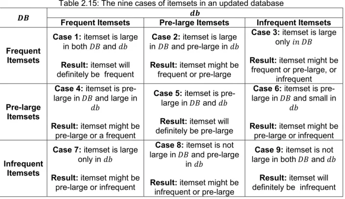
traditional algorithms. The second threshold stands for identifying the pre-large itemsets. Based on this solution, an itemset may have the nine cases summarized in table 2.15.
Table 2.15: The nine cases of itemsets in an updated database
𝑫𝑩 Frequent Itemsets Pre-large Itemsets𝒅𝒃 Infrequent Itemsets
Frequent Itemsets
Case 1: itemset is large
in both 𝐷𝐵 and 𝑑𝑏
Result: itemsetwill definitely be frequent
Case 2: itemset is large
in 𝐷𝐵 and pre-large in 𝑑𝑏
Result: itemsetmight be frequent or pre-large
Case 3: itemset islarge
only 𝑖𝑛 𝐷𝐵
Result: itemsetmight be frequent or pre-large, or
infrequent Pre-large
Itemsets
Case 4: itemset is
pre-large in 𝐷𝐵 and large in
𝑑𝑏
Result: itemsetmight be pre-large or a frequent
Case 5: itemset is pre-
large in 𝐷𝐵 and 𝑑𝑏
Result: itemsetwill definitely be pre-large
Case 6: itemset is pre-
large in 𝐷𝐵 and small in
𝑑𝑏
Result: itemsetmight be pre-large or infrequent Infrequent
Itemsets
Case 7: itemset is large
only in 𝑑𝑏
Result: itemsetmight be pre-large or infrequent
Case 8: itemset is not
large in 𝐷𝐵 and pre-large
in 𝑑𝑏
Result: itemsetmight be infrequent or pre-large
Case 9: itemset is not
large in both 𝐷𝐵 and 𝑑𝑏
Result: itemsetwill definitely be infrequent
Among the nine cases, both case 1 and case 9 will change nothing in the existing association rules. Also, Case 2, Case 3, and Case 4 can be handled effectively, and can be determined by retaining all frequent and pre-large itemsets with their supports in the old database. For case 7, it is unlikely for an itemset to be large in the updated database since the fraction of the number 𝑑𝑏 over the number of 𝐷𝐵 is usually trivial.
2.2 Association Rules Mining on Uncertain Data
Traditional association rules maiming algorithms assume a transactional database where for each transaction we know for sure the items that belong to the transaction. In
19
many real life applications, the database is uncertain, and for any transaction, we only know a probability for each possible item that this item belongs to the transaction [40]. In this case the frequency of an item (or an itemset) is calculated as the expected number of occurrences of the item (itemset) in the transactions [41, 39]. Research has also been conducted to mine rules from uncertain data [40-46] due to the growth of applications that involve uncertain data such as data from social networks, sensor networks [47], protein-protein interaction analysis [48], and inaccurate surveys. Uncertainty could arise from masking of data for privacy concerns as well [49].
Definition 2.4: The problem of mining from uncertain data can be formulated as follows. Let the set of distinct items be 𝐼 = {𝑖1, 𝑖2, … , 𝑖𝑚}. Consider an uncertain database 𝑈𝐷𝐵 which contains a set of 𝑁 transactions, 𝑇 = {𝑡1, 𝑡2, … , 𝑡𝑁}.. Here the transaction 𝑡𝑗is characterized as a probability vector 𝑝𝑗(𝑖1), 𝑝𝑗(𝑖2), ⋯ , 𝑝𝑗(𝑖𝑚) where 𝑝𝑗(𝑥) is the probability
that the transaction 𝑡𝑗 contains the item 𝑥, for any item 𝑥 and 1 ≤ 𝑗 ≤ 𝑁. Let X be any
itemset. We can define the expected support of 𝑋 as follows.
Definition 2.5: Let 𝑈𝐷𝐵 be an uncertain database with 𝑁 transactions, and let 𝑋
be any itemset. Then, the expected support of 𝑋 is given by the following equation:
𝑒𝑠𝑢𝑝(𝑋) =∑𝑁 ∏𝑥∈𝑋 𝑝𝑗(𝑥)
𝑗=1 .
Definition 2.6: An itemset 𝑋 is said to be frequent if and only if its expected support
𝑒𝑠𝑢𝑝(𝑋) is atleast (𝑁 × 𝑚𝑖𝑛𝑠𝑢𝑝) where 𝑁 is the number of transactions and 𝑚𝑖𝑛𝑠𝑢𝑝 is the minimum expected support required and it is specified by the user.
20
Example 2.6: Table 2.16 shows a small 𝑈𝐷𝐵 where each row represents one transaction. If 𝑡 is any transaction, then all the items in this transaction that have a nonzero probability of occurrence are listed in column 2 of the corresponding row. Since the itemset {𝑎, 𝑏} appears only in one transaction 𝑡1, then 𝑒𝑠𝑢𝑝({𝑎, 𝑏}) = [0.1033 × 0.865] = 0.08935. Also, since the itemset {𝑏, 𝑑} appears together in 𝑡1, 𝑡2 and 𝑡3, then
𝑒𝑠𝑢𝑝({𝑏, 𝑑}) = [(0.865 × 0.726) + (0.906 × 0.726 ) + (0.882 × 0.897)] = 2.0769. If
𝑚𝑖𝑛𝑠𝑢𝑝 is given as 0.3, then the itemset {𝑏, 𝑑} qualifies as a frequent itemset (based on the expected support) whereas the itemset {𝑎, 𝑏} does not qualify.
Table 2.16: An uncertain database
TID Transactions
𝒕𝟏 a (0.1033) b (0.865) c (0.919) d (0.726)
𝒕𝟐 c (0.854) b (0.906) d (0.726)
𝒕𝟑 b(0.882) e(0.853) d(0.897)
2.2.1 Frequent patterns Algorithms for Uncertain Data
Most of the frequent patterns algorithms under uncertainty, are extended versions of those traditional rules mining algorithms with certain data. For example, UApriori which extends the traditional Apriori algorithm is first algorithm introduced for finding frequent itemsets based on expected support in uncertain databases. Chui, et al. [45] have introduced the UApriori algorithm that is based on the computation of expected supports. Like the traditional Apriori, it adapts a support-based frequent itemsets recursively. In uncertain databases, downward closure property [8] also is satisfied. So, we still can prune all the supersets of expected support-based infrequent itemsets. Chui, et al. [45] have also proposed decremental pruning methods to improve the efficiency of UApriori. The decremental pruning methods are employed to estimate an upper bound on the
21
expected support of an itemset from the beginning, and the traditional Apriori pruning is used when the upper bound is lower than the minimum expected support. Yet, the traditional Apriori pruning is mainly used in UApriori since the decremental pruning methods depend on the structure of the datasets.
UFP-growth [46] is similar to the certain FP-growth algorithm. It first builds a compact data structure called the UFP-tree using only two passes over the uncertain database. Then, it constructs conditional sub-trees and finds expected support-based frequent itemsets from the UFP-tree. Unlike FP-growth, where the compact FP-tree shrinks different transactions that share common subsets/prefixes in only one path, UFP-tree is substantially reduced. Thus, items may share only one node when both their ids and probabilities are common. Otherwise, even common subsets/prefixes that don’t share the same probabilities will be represented in two different nodes/paths. Due to fewer shared nodes and paths, an uncertain database can be viewed as a sparse database. A lot of redundant computations take place while processing a UFP-tree since the number of conditional sub-trees could be very large. In fact, the performance of the deterministic FP-growth cannot be achieved using UFP-growth.
Leung, et al. [47] have suggested a straightforward solution by considering each distinct probability as a different item. This solution can be effective only when many items have the same probability which is not the typical case in the domain of uncertain databases [41]. Agarwal, et al. [41] suggested another solution by creating clustered ranges of probabilities and for each clustered range the relevant nodes are linked. Followed by this, FP-Tree algorithm is used to generate a close superset of the frequent
22
itemsets. They also suggested another solution by using an extended H-Mine, namely, U H-Mine [41].
Unlike the traditional Apriori algorithm in deterministic databases, the performance of UApriori is better than the other mining algorithms in the domain of uncertain data. It is considered as one of the fastest for dense uncertain datasets in general [41].
23
Chapter 3
Frequent Itemsets Mining From Weighted
Uncertain Data
3.1 Introduction
Mining frequent itemsets from datasets is a well-studied problem. Traditional approaches to mining frequent patterns have suffered from the fact that all the items are treated as equally important. In real applications, each item has a different level of importance. For example, in retail applications some products may be much more expensive than the others, and these expensive items may not be present in a large number of transactions. The importance of weight-based pattern mining approach can be felt in many domains such as, biomedical data analysis where the causes of most diseases are not only one gene but a combination of genes; web traversal pattern mining where the impact of each web page is different; and so on. Several variations of this problem have also been investigated in the literature [50-54]. On the other hand, there are many applications where the data are both weighted and uncertain. To the best of our knowledge, mining from such datasets has not been studied before. In this research work
24
we initiate the study of frequent itemsets mining from weighted uncertain data. In particular, we propose two algorithms called 𝐻𝑊𝑈𝐴𝑃𝑅𝐼𝑂𝑅𝐼 and 𝑉𝑊𝑈𝐹𝐼𝑀 for mining frequent itemsets from weighted uncertain data [55]. We evaluate the performance of the proposed algorithms on various datasets.
Definition 3.1: Let 𝑤(𝐼) be a positive real number that stands for the weight of an item. It represents the importance of the item in the transaction database. Then, the weight of an itemset 𝑋 is the average weight of items, and is defend as:
𝑊(𝑋) = ∑𝑙𝑒𝑛𝑔𝑡ℎ (𝑋)1 𝑤𝑋 𝑙𝑒𝑛𝑔𝑡ℎ (𝑋) .
Definition 3.2: Weighted support of an itemset is defined as:
𝑊𝑠𝑢𝑝𝑝𝑜𝑟𝑡(𝑋) = 𝑊(𝑋) × 𝑆𝑢𝑝𝑝𝑜𝑟𝑡 (𝑋).
Definition 3.3: An itemset 𝑋 is said to be a weighted frequent pattern if
𝑊𝑠𝑢𝑝𝑝𝑜𝑟𝑡(𝑋) ≥ 𝑚𝑖𝑛𝑠𝑢𝑝.
Many algorithms have been proposed for weighting items based on their significance. Unfortunately, the 𝑑𝑜𝑤𝑛𝑤𝑎𝑟𝑑 𝑐𝑙𝑜𝑠𝑢𝑟𝑒 𝑝𝑟𝑜𝑝𝑒𝑟𝑡𝑦 does not hold for weighted data making it a challenge to develop mining algorithms [1].
Example 3.1: Table 3.1 shows a small certain data, where each transaction has a subset of items, and each item is assigned with weight in table 3.2. Assume that the minimum threshold, 𝑚𝑖𝑛𝑠𝑢𝑝 = 0.5. Weighted support for pattern diaper is
25
𝑊𝑠𝑢𝑝𝑝𝑜𝑟𝑡(diaper) = 0.6 ×34 = 0.45 < 𝑚𝑖𝑛𝑠𝑢𝑝, while weighted support for each pattern
(𝑒𝑔𝑔,diaper) is 𝑊𝑠𝑢𝑝𝑝𝑜𝑟𝑡(𝑒𝑔𝑔,diaper) =(0.5 + 0.6)2 ×44 = 0.55 > 𝑚𝑖𝑛𝑠𝑢𝑝. However, if we follow the rule of 𝑑𝑜𝑤𝑛𝑤𝑎𝑟𝑑 𝑐𝑙𝑜𝑠𝑢𝑟𝑒 𝑝𝑟𝑜𝑝𝑒𝑟𝑡𝑦 we will delete item (𝑑𝑖𝑎𝑝𝑒𝑟) in the early stage, and we will lose the itemset (𝑒𝑔𝑔,𝑑𝑖𝑎𝑝𝑒𝑟) that has a weighted support greater than
the 𝑚𝑖𝑛𝑠𝑢𝑝. As we can see using weights violates the well-known
𝑑𝑜𝑤𝑛𝑤𝑎𝑟𝑑 𝑐𝑙𝑜𝑠𝑢𝑟𝑒 𝑝𝑟𝑜𝑝𝑒𝑟𝑡𝑦 that has a great impact on reducing search space, and time.
Table 3.1: Certain data for example 3.1
TID Transactions
𝑇1 milk, egg, diaper, beer
𝑇2 egg, diaper, beer
𝑇3 egg, diaper, beer, chees
𝑇4 egg, diaper
Table 3.2: Items’ weights for example 3.1
Items Weight milk 0.6 egg 0.5 diaper 0.6 beer 0.5 chees 0.1
3.2 Weighted frequent pattern mining algorithms on
certain database
Both WARM [51], and WAR [52] were proposed based on the Apriori algorithm which is a level-wise approach to generate weighted association rules. The authors of WARM [51] introduced two varieties of weight; a weight assigned for each individual item, and an itemset weight. The itemset weight is the average weight of the items. An interesting rule has to satisfy the support and confidence thresholds, and the weighted support has to be at least a user-defined threshold weighted minimum support called 𝑤𝑚𝑖𝑛𝑠𝑢𝑝. The
26
weighted support is the fraction of the transactions’ weight (that contains itemset) relative to the total transactions’ weight.
Example 3.2: using items’ weight in table 3.2 each individual item is assigned with weight. Table 3.3 shows a small certain data, where the weight for each transaction is calculated in the column 𝑇𝑊𝑒𝑖𝑔ℎ𝑡, (i.e. weight of transaction 𝑇1= 0.6+0.5+0.6+0.5+0.15 = 0.46).
Assume that both minimum threshold 𝑚𝑖𝑛𝑠𝑢𝑝 = 0.5, and weighted minimum threshold
𝑤𝑚𝑖𝑛𝑠𝑢𝑝 = 0.5. Support for pattern (𝑒𝑔𝑔,diaper) is 𝑠𝑢𝑝(𝑒𝑔𝑔,diaper) =3
4 = 0.75 > 𝑚𝑖𝑛𝑠𝑢𝑝, and weighted support for pattern (𝑒𝑔𝑔,diaper) is 𝑊𝑠𝑢𝑝𝑝𝑜𝑟𝑡(𝑒𝑔𝑔,diaper) = 0.46+ 0.53+ 0.425
2.015 = 0.70 > 𝑤𝑚𝑖𝑛𝑠𝑢𝑝
Table 3.3: Weighed transactional certain data for example 3.2
TID Transactions TWeight
𝑇1 milk, egg, diaper, beer, chees 0.46
𝑇2 egg, diaper, beer 0.53
𝑇3 egg, diaper, beer, chees 0.425
𝑇4 diaper 0.6
Total transaction weight 2.015
Giving a weight range for each individual item, WAR [52] starts by generating the frequent itemsets using the traditional Apriori algorithm without considering item/itemset weight. It then, generates the weighted association rules under three conditions; weighted association rule has to satisfy both support and confidence thresholds, and new measurement called density threshold using space partition. Yun, et al. [53] have proposed
𝑊𝐹𝐼𝑀 as the first algorithm based on FP-tree growth algorithm for frequent itemset mining from weighted data. Similar to FP-tree growth algorithm, 𝑊𝐹𝐼𝑀 scans the database twice. In order to ensure the 𝑑𝑜𝑤𝑛𝑤𝑎𝑟𝑑 𝑐𝑙𝑜𝑠𝑢𝑟𝑒 𝑝𝑟𝑜𝑝𝑒𝑟𝑡𝑦, a minimum weight and a weight range
27
are used, where each item has a random fixed weight 𝑊 in a weight range: 𝑊𝑚𝑖𝑛≤ 𝑊 ≤ 𝑊𝑚𝑎𝑥. An itemset X is a weighted infrequent itemset if, following pruning, condition 1 or
condition 2 below is satisfied:
1. Pruning condition 1: 𝑠𝑢𝑝(𝑋) < 𝑚𝑖𝑛𝑠𝑢𝑝 && 𝑊(𝑋) < 𝑊𝑚𝑖𝑛
2. Pruning condition 2: 𝑊𝑠𝑢𝑝(𝑋) < 𝑚𝑖𝑛𝑠𝑢𝑝, where 𝑊𝑠𝑢𝑝(𝑋) = 𝑠𝑢𝑝(𝑋) × 𝑊𝑚𝑖𝑛
Here 𝑠𝑢𝑝(𝑋) stands for the support of 𝑋, 𝑚𝑖𝑛𝑠𝑢𝑝 is the minimum support threshold, 𝑊(𝑋)is the average weight of the items in 𝑋, 𝑊𝑚𝑖𝑛is the minimum weight, and𝑊𝑠𝑢𝑝(𝑋) is weighted support.
Yun [54] has proposed an algorithm called 𝑊𝐼𝑃 based on the FP-tree growth algorithm. He has also defined the concept of a weighted ℎ𝑦𝑝𝑒𝑟𝑐𝑙𝑖𝑞𝑢𝑒. This is a new measure of weight-confidence that measures the weight affinity of a pattern and prevents the generation of patterns that have significantly different weight levels. Weight confidence of a pattern 𝑋 = {𝐼1, 𝐼2, 𝐼3, … , 𝐼𝑚} is defined as the ratio of the minimum weight of items to the maximum weight of items:
𝑊𝑐𝑜𝑛𝑓(𝑋) = 𝑀𝑖𝑛 1≤𝑖≤𝑚 {weight({Ii})} 𝑀𝑎𝑥 1≤𝑗≤𝑚 {weight({Ij})}.
If the weight confidence of a pattern is greater than or equal to a minimum weight confidence, then the pattern is called a weighted ℎ𝑦𝑝𝑒𝑟𝑐𝑙𝑖𝑞𝑢𝑒 pattern. An itemset 𝑋 is a weighted infrequent itemset if, following pruning, condition 1 or condition 2 or condition 3 below is satisfied:
1. Pruning condition 1: 𝑠𝑢𝑝(𝑋) × 𝑊𝑚𝑖𝑛 < 𝑚𝑖𝑛𝑠𝑢𝑝
28
3. Pruning condition 3: ℎ𝑐𝑜𝑛𝑓𝑖𝑑𝑒𝑛𝑐𝑒 < 𝑚𝑖𝑛ℎ𝑐𝑜𝑛𝑓, where, the ℎ − 𝑐𝑜𝑛𝑓𝑖𝑑𝑒𝑛𝑐𝑒 of a pattern 𝑋 = {𝐼1, 𝐼2, 𝐼3, … , 𝐼𝑚} is defined as: 𝑀𝑎𝑥 support ({𝐼1,𝐼2,𝐼3,…,𝐼𝑚})
1≤𝑗≤𝑚 {𝑠𝑢𝑝𝑝𝑜𝑟𝑡 ({Ij})}.
3.3 Proposed Algorithms of Weighted frequent pattern
mining algorithms on uncertain data
In this section we present elegant algorithms for mining weighted frequent itemsets from uncertain databases. In the 𝑊𝐹𝐼𝑀 algorithm [53], for the case of certain data, an itemset
𝑋 is a weighted infrequent itemset if, following pruning, condition 1 or condition 2 below is satisfied:
1. Pruning condition 1: 𝑠𝑢𝑝(𝑋) < 𝑚𝑖𝑛𝑠𝑢𝑝 && 𝑊(𝑋) < 𝑊𝑚𝑖𝑛
2. Pruning condition 2: 𝑊𝑠𝑢𝑝(𝑋) < 𝑚𝑖𝑛𝑠𝑢𝑝, where 𝑊𝑠𝑢𝑝(𝑋) = 𝑠𝑢𝑝(𝑋) × 𝑊𝑚𝑖𝑛
Therefore, in uncertain data, we can say, an itemset is frequent if both following pruning conditions are not satisfied:
1. Pruning condition 1: 𝑒𝑠𝑢𝑝(𝑋) < 𝑚𝑖𝑛1𝑒𝑠𝑢𝑝 && 𝑊(𝑋) < 𝑊𝑚𝑖𝑛
2. Pruning condition 2: 𝑊𝑒𝑠𝑢𝑝(𝑝) [= 𝑒𝑠𝑢𝑝(𝑋) × 𝑊(𝑋)] < 𝑚𝑖𝑛2𝑒𝑠𝑢𝑝
Where 𝑒𝑠𝑢𝑝 is the expected support, and 𝑊𝑒𝑠𝑢𝑝 is the weighted expected support. We introduce two support parameters 𝑚𝑖𝑛1𝑒𝑠𝑢𝑝 and 𝑚𝑖𝑛2𝑒𝑠𝑢𝑝, where𝑚𝑖𝑛1𝑒𝑠𝑢𝑝 stands for the first pruning condition, and 𝑚𝑖𝑛2𝑒𝑠𝑢𝑝stands for the second pruning condition. Also, 𝑚𝑖𝑛2𝑒𝑠𝑢𝑝 should be less than 𝑚𝑖𝑛1𝑒𝑠𝑢𝑝. Our algorithms for weighted uncertain frequent
itemset mining are designed using two layouts namely ℎ𝑜𝑟𝑖𝑧𝑜𝑛𝑡𝑎𝑙 and 𝑣𝑒𝑟𝑡𝑖𝑐𝑎𝑙.
𝐻𝑜𝑟𝑖𝑧𝑜𝑛𝑡𝑎𝑙 𝐿𝑎𝑦𝑜𝑢𝑡 of any dataset keeps the data as transactions where each transaction is an itemset. On the other hand, the 𝑣𝑒𝑟𝑡𝑖𝑐𝑎𝑙 𝑙𝑎𝑦𝑜𝑢𝑡 keeps the data as a list of
29
transactions for each item. The list associated with any item is the list of transactions in which the item is present. Below we present the horizontal weighted uncertain Apriori algorithm.
Example 3.3: Consider the uncertain transaction database UDB shown in Table 3.4. Table 3.5 shows each individual item is assigned with weight. Note just for testing, we give some item that has low support, high weight and via versa. Let 𝑚𝑖𝑛𝑠𝑢𝑝1 = 0.5 , 𝑊𝑚𝑖𝑛 = 0.1, andnumber of tranactions 𝑁 = 3.
Table 3.4: uncertain transaction database for example 3.3
TID Transactions
𝑇1 1 0.933 2 0.865 3 0.919 4 0.726
𝑇2 2 0.854 3 0.906 4 0.726
𝑇3 3 0.933 4 0.865 5 0.919
Table 3.5: Item’s weight for example 3.3
Items Weight 1 0.9 2 0.6 3 0.2 4 0.5 5 0.1 𝑚𝑖𝑛1𝑒𝑠𝑢𝑝= 𝑁 × 𝑚𝑖𝑛𝑠𝑢𝑝1= (3 × 0.5) = 1.5, and 𝑚𝑖𝑛2𝑒𝑠𝑢𝑝= 𝑚𝑖𝑛1𝑁𝑒𝑠𝑢𝑝 = (1.53) = 0.5 𝑒𝑠𝑢𝑝 (1) = 0.9 < 𝑚𝑖𝑛1𝑒𝑠𝑢𝑝 𝑒𝑠𝑢𝑝 (2) = 0.865 + 0.854 = 1.7 > 𝑚𝑖𝑛1𝑒𝑠𝑢𝑝 𝑒𝑠𝑢𝑝 (3) = 0.919 + 0.906 + 0.933 = 2.758 > 𝑚𝑖𝑛1𝑒𝑠𝑢𝑝 𝑒𝑠𝑢𝑝 (4) = 0.726 + 0.726 + 0.865 = 2.317 > 𝑚𝑖𝑛1𝑒𝑠𝑢𝑝 𝑒𝑠𝑢𝑝 (5) = 0.919 < 𝑚𝑖𝑛1𝑒𝑠𝑢𝑝
According to Pruning condition 1, 𝑒𝑠𝑢𝑝 (5) = 0.919 < 𝑚𝑖𝑛1𝑒𝑠𝑢𝑝 && 𝑊(5) < 𝑊𝑚𝑖𝑛.
30 According to Pruning condition 2,
𝑊𝑠𝑒𝑢𝑝(1) = 0.9 × 0.933 = 0.8 > 𝑚𝑖𝑛2𝑒𝑠𝑢𝑝
𝑊𝑠𝑒𝑢𝑝(2) = 0.6 × (0.865 + 0.854) = 0.6 × 1.719 = 1.03 > 𝑚𝑖𝑛2𝑒𝑠𝑢𝑝
𝑊𝑠𝑒𝑢𝑝(3) = 0.2 × (0.919 + 0.906 + 0.933) = 0.2 × 2.758 = 0.5516 > 𝑚𝑖𝑛2𝑒𝑠𝑢𝑝
𝑊𝑠𝑒𝑢𝑝(4) = 0.5 × (0.726 + 0.726 + 0.865) = 0.5 × 2.317 = 1.1585> 𝑚𝑖𝑛2𝑒𝑠𝑢𝑝
Let return item (5) to test the downward closure property: 𝑊(1,2) = [0.9 + 0.62 ] = 0.75 > 𝑊𝑚𝑖𝑛 𝑊(1,3) = [0.9 + 0.22 ] = 0.5> 𝑊𝑚𝑖𝑛 𝑊(1,4) = [0.9 + 0.52 ] = 0.7 > 𝑊𝑚𝑖𝑛 𝑊(2,3) = [0.6 + 0.32 ] = 0.45 > 𝑊𝑚𝑖𝑛 𝑊(2,4) = [0.6 + 0.52 ] = 0.55 > 𝑊𝑚𝑖𝑛 𝑊(3,4) = [0.2 + 0.52 ] = 0.35 > 𝑊𝑚𝑖𝑛 𝑊(3,5) = [0.2 + 0.12 ] = 0.15 > 𝑊𝑚𝑖𝑛 𝑊(4,5) = [0.5 + 0.12 ] = 0.3 > 𝑊𝑚𝑖𝑛 And: 𝑒𝑠𝑢𝑝 (1,2) = 0.8 < 𝑚𝑖𝑛1𝑒𝑠𝑢𝑝 But, 𝑊(1,2) > 𝑊𝑚𝑖𝑛 𝑒𝑠𝑢𝑝 (1,2) 𝑓𝑟𝑒𝑞𝑢𝑛𝑡 𝑒𝑠𝑢𝑝 (1,3) = 0.9 < 𝑚𝑖𝑛1𝑒𝑠𝑢𝑝 But, 𝑊(1,3) > 𝑊𝑚𝑖𝑛 𝑒𝑠𝑢𝑝 (1,3) 𝑓𝑟𝑒𝑞𝑢𝑛𝑡 𝑒𝑠𝑢𝑝 (1,4) = 0.7 < 𝑚𝑖𝑛1𝑒𝑠𝑢𝑝 But, 𝑊(1,4) > 𝑊𝑚𝑖𝑛 𝑒𝑠𝑢𝑝 (1,4) 𝑓𝑟𝑒𝑞𝑢𝑛𝑡 𝑒𝑠𝑢𝑝 (2,3) = 1.6 > 𝑚𝑖𝑛1𝑒𝑠𝑢𝑝 And, 𝑊(2,3) > 𝑊𝑚𝑖𝑛 𝑒𝑠𝑢𝑝 (2,3) 𝑓𝑟𝑒𝑞𝑢𝑛𝑡 𝑒𝑠𝑢𝑝 (2,4) = 1.2 < 𝑚𝑖𝑛1𝑒𝑠𝑢𝑝But, 𝑊(2,4) >𝑊𝑚𝑖𝑛 𝑒𝑠𝑢𝑝 (2,3) 𝑓𝑟𝑒𝑞𝑢𝑛𝑡 𝑒𝑠𝑢𝑝 (3,4) = 2.1 > 𝑚𝑖𝑛1𝑒𝑠𝑢𝑝And, 𝑊(3,4) > 𝑊𝑚𝑖𝑛 𝑒𝑠𝑢𝑝 (3,4) 𝑓𝑟𝑒𝑞𝑢𝑛𝑡 𝑒𝑠𝑢𝑝 (3,5) = 0.9 < 𝑚𝑖𝑛1𝑒𝑠𝑢𝑝And 𝑊(3,5) > 𝑊𝑚𝑖𝑛 𝑒𝑠𝑢𝑝 (3,5) 𝑓𝑟𝑒𝑞𝑢𝑛𝑡