Institute of Parallel and Distributed Systems University of Stuttgart
Universitätsstraße 38 D–70569 Stuttgart
Masterarbeit Nr. 63
Predicting the GPU Execution Time
of 3D Rendering Commands using
Machine Learning Concepts
Robin KellerCourse of Study: Informatik
Examiner: Prof. Dr. Kurt Rothermel
Supervisor: Dipl.-Inf. Stephan Schnitzer
Commenced: November 2, 2015
Abstract
3D rendering gets more and more important in embedded environments like automotive industry. To reduce hardware costs, power consumptions, and installation space for Electronic Control Units (ECUs), the ECUs including their GPU are consolidated. Thus, multiple applications with diverse requirements use the same GPU. For example, the speedometer has safety-critical requirements, whereby third party application does not. To execute multiple applications on the GPU a GPU scheduler is necessary. So far, GPUs do not support preemption and thus, a non preemptive real-time GPU scheduling is required. Such a real-time GPU scheduler needs the execution time of GPU commands beforehand. Predicting the GPU execution time is complex and hence, we tackle this problem by using machine learning concepts to predict the execution time of GPUs. In this thesis, influence factors for the execution time of 3D rendering commands on the GPU are analyzed and how these factors are processed to use them as features for the online machine learning algorithm. This leads to a linear regression problem that is tackled by using stochastic gradient descent with online normalization of the input data and an adaptive learning rate calculation. Furthermore, the shaders are analyzed during runtime and the feature vector contains the GPU instructions. This allows the algorithm to gain knowledge about the execution time for so far unseen shaders. To validate the concept, it is implemented and evaluated on a workstation computer and on an embedded board. We show for the workstation computer that the newly developed concept has higher accuracy in glmark2-es2 benchmarks than the previous approach. For the embedded board is shown that the execution times for GPU instructions can be learned accurately. However, the developed concept provides room for improvement at constant scenes, where only the execution time changes.
3D-Rendering wird in eingebetteten Umgebungen, wie zum Beispiel der Automobilin-dustrie, zunehmend wichtiger. Um die Hardwarekosten, den Energieverbrauch und den Einbauraum von Steuergeräten zu reduzieren, sollen die Steuergeräte einschließlich ihrer GPU konsolidiert werden. So verwenden mehrere Anwendungen mit unterschiedlichen Anforderungen dieselbe GPU. Zum Beispiel weist der Tachometer sicherheitskritische Anforderungen auf, wobei Drittanbieter-Anwendungen diese nicht besitzen. Zur Aus-führung mehrerer Anwendungen auf der GPU ist ein GPU-Scheduler notwendig. Bisher unterstützen GPUs keine Preemption, sodass ein preemptiver GPU-Scheduler, welcher Echtzeitanforderungen erfüllt, erforderlich ist. Ein solcher Echtzeit-GPU-Scheduler benötigt im Voraus die Ausführungszeit der GPU-Befehle. Um die GPU-Ausführungszeit vorherzusagen, wird in dieser Arbeit ein Vorhersage-Framework entworfen, welches maschinelles Lernen verwendet.
In dieser Arbeit werden Einflussfaktoren auf die Ausführungszeit von 3D-Rendering-Befehlen auf der GPU analysiert. In diesem Zusammenhang wird aufgezeigt, wie diese Faktoren verarbeitet werden, um sie als Features für den Algorithmus zu verwenden, der zur Laufzeit maschinelles Lernen einsetzt. Dieses führt zu einer linearen Regressions-analyse, welche durch die Verwendung des Gradientenverfahrens mit Normalisierung der Eingabedaten zur Laufzeit und adaptiver Lernratenberechnung angegangen wird. Außerdem werden die verwendeten Shader zur Laufzeit analysiert und die ermittelten GPU-Instruktionen in den Feature Vektor aufgenommen. Das erlaubt dem Algorithmus, Wissen über die Ausführungszeit von bisher unbekannten Shadern zu erlangen. Um das Konzept zu validieren, wurde es auf einer Workstation und einem eingebetteten Board implementiert und evaluiert. In der Evaluation wird dargestellt, dass für die Workstation das neu entwickelte Konzept eine höhere Genauigkeit in glmark2-es2 Benchmark-Tests besitzt als in dem bisherigen Ansatz. Für das eingebettete Board wird gezeigt, dass die Ausführungszeiten für GPU-Instruktionen präzise gelernt werden können. Jedoch bietet das entwickelte Konzept Raum für Verbesserungen bei konstanten Szenen, in denen sich nur die Ausführungszeiten verändern.
Contents
1 Introduction 1 1.1 Motivation . . . 1 1.2 Contribution . . . 2 1.3 Outline . . . 3 2 Related Work 5 2.1 GPU Scheduling and Execution Time Prediction . . . 52.2 Online Learning: Stochastic Gradient Descent . . . 6
3 Background 9 3.1 OpenGL ES 2.0 . . . 9
3.2 Machine Learning . . . 14
4 Concept 21 4.1 Selection of Features . . . 21
4.2 Learning on GPU Instruction Level . . . 23
4.3 Linear Model . . . 25
4.4 Prediction Framework . . . 27
4.5 Online Learning . . . 30
4.6 Store the Model Parameters . . . 36
5 Implementation 39 5.1 Setup . . . 39 5.2 Interception Layer . . . 40 5.3 Machine Learning . . . 44 5.4 Shader Analyzer . . . 47 5.5 Linear Regression . . . 48 6 Evaluation 53 6.1 Setup . . . 53
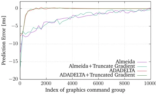
6.2 Choice of Stochastic Gradient Descent Setup . . . 53
7.2 Future Work . . . 68
A Appendix 69
A.1 Vivante Opcodes . . . 69 A.2 Tesla Instruction Set Architecture . . . 69
List of Figures
3.1 OpenGL ES 2.0 Processing Pipeline [8, p. 13] . . . 10 4.1 Architecture of the Prediction Framework . . . 27 4.2 Execution Time Prediction using Machine Learning . . . 29 6.1 Convergence of machine learning algorithms using the application
"shadergen" on the Nvidia GPU. . . 55 6.2 Convergence of machine learning algorithms using the application
"shadergen" on the Vivante GPU. . . 56 6.3 Nvidia: Comparing accuracy of machine learning algorithms using the
program "shadergen". . . 57 6.4 Vivante: Comparing accuracy of machine learning algorithms using the
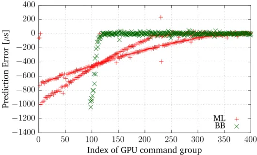
program "shadergen". . . 57 6.5 Adaptivity of the bounding box and machine learning algorithm using
glmark2-es2 "buffer" on the Nvidia graphics card. . . 61 6.6 Adaptivity of the bounding box and machine learning algorithm using
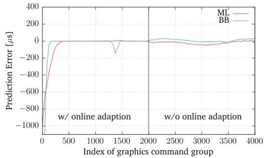
glmark2-es2 "buffer" on the Vivante graphics card. . . 62 6.7 Vivante: Learning the model parameters using glmark2-es2 "buffer". . . 63 6.8 Cumulative distribution function of the error of machine learning and
bounding box algorithm for the Nvidia graphics card. . . 65 6.9 Cumulative distribution function of the error of machine learning and
4.1 Tesla ISA instruction type [24] . . . 24
6.1 Estimated Execution Time of Nvidia GPU Instructions . . . 58
6.2 Estimated Execution Time of Vivante GPU Instructions . . . 58
A.1 Tesla opcode map part 1/2 adapted from [24]. . . 70
List of Algorithms
4.1 Stochastic gradient descent . . . 31
4.2 Normalization used by stochastic gradient descent . . . 32
4.3 Learning rate calculation based on Almeida et al. . . 33
4.4 Learning rate calculation based on ADADELTA . . . 34
4.5 Weight update for online learning . . . 36
5.1 General interception of OpenGL calls . . . 40
5.2 Interception of eglCreateContext . . . 41
5.3 Interception of glDrawArrays . . . 41
5.4 Predicting the execution time at the end of each command group . . . . 42
5.5 Interception of glClear . . . 43
5.6 Predicting the execution time for one command group . . . 44
5.7 Add new samples to the machine learning module . . . 45
5.8 Transformation of the state into the feature vector . . . 46
5.9 Predicting the execution time . . . 46
5.10 Using the measured execution time to learn the model parameters . . . . 47
5.11 Creating the distribution of GPU instruction for a program . . . 47
5.12 Predicting the execution time . . . 48
5.13 Learning the model parameters using stochastic gradient descent . . . . 49
5.14 Implementation of the learning rate calculation based on Almeida et al. . 50
5.15 Implementation of the learning rate calculation based on ADADELTA . . 51
1 Introduction
In this chapter, the work at this topic is motivated, the contribution in this research area and the organization of this thesis is presented.
1.1 Motivation
Nowadays, graphics processing units (GPU) are integrated into embedded systems to use high resolution 3D rendering. The number of displays in embedded systems increases, which leads to a greater demand of GPUs, that are required to control the displays. In embedded systems, usually, each electronic control unit (ECU) contains one GPU. Therefore, with a higher number of display, the number of ECUs increases as well. In the automotive industry, the cars are using more and more displays to show high resolution 3D graphics.
To reduce cost, energy and space requirements in a setup with multiple ECUs, the ECUs can be consolidated. However, that means, that multiple 3D rendering tasks need to run on one ECU in parallel. That leads to the fact, that multiple 3D rendering tasks must run on one GPU. To run multiple 3D rendering tasks on one GPU, a GPU scheduler is necessary.
Another aspect that needs to be considered for consolidating ECUs is that, 3D rendering tasks can have real-time requirements. For example, in the case of the automotive domain, in high class cars the instrument cluster containing the tachometer is displayed with 3D rendering commands and has real-time requirements. Other 3D graphics applications, which run on the same GPU, can be infotainment or third party applications. If there is at least one 3D rendering task with real-time requirements running on the GPU, the system needs to handle real-time requirements.
This leads to a setup, in which a real-time GPU scheduler is required. Because of the fact that the GPU is not a preemptive system, a started 3D rendering job on the GPU cannot be interrupted and needs to be finished before another 3D rendering job can be started. Therefore, such a real-time GPU scheduler needs the execution time of each
task beforehand. Existing real-time GPU schedulers such as [22] depend on accurate execution time prediction.
However, prediction of the execution time of 3D rendering commands is complex. To determine the execution time of 3D rendering commands, the rendering can be emulated on the central processor unit (CPU). The predicted execution time is accurate, but the calculation of the execution time takes much more time than executing the 3D rendering job on the GPU. On the other hand, the execution time can be estimated by only using the raw input data of the 3D rendering command. Thus, the time to estimate the execution time is reasonable, but the accuracy of the prediction is insufficient. Thus, a trade-off between calculating some parts of the 3D rendering command and estimating other parts needs to be find.
Kato et al. [3] and Yu et al. [26] proposed history based approaches to predict the execution time of GPU command groups. If the GPU command group data varies, the results of the history based approach are insufficient accurate. Schnitzer et al. [21] use the tracked OpenGL context to predict the execution time of GPU command groups. A downside for this approach is, that for each shader a calibration is needed. A prediction cannot be performed during the calibration, because the calibrated values are uncertain and the predicted execution time would be inaccurate.
This motivates us to propose a concept which improves the previous approaches. This can be done by getting rid of the calibration for new shaders and being adaptive to varying environments using a self-tuning machine learning. Thus, our machine learning algorithm leads to higher flexibility and faster adaption of the real world. However, OpenGL is a complex state based graphics rendering environment, which does not provide all necessary information for machine learning. Another challenge is the embedded system setting, in which less computation power is provided. Therefore, stochastic gradient descent is applied which leads to more challenges.
1.2 Contribution
In this section, an overview of the main contributions of this work is presented. In general, to predict the execution time, the influence factors need to be analyzed. Using the measured execution time and the influence factors of past 3D rendering commands, machine learning is applied to learn the underlying model parameters.
1. Using the influence factors of the execution time of 3D rendering commands using OpenGL, the features for machine learning are determined and presented. Furthermore, a linear function which describes the execution time is presented.
1.3 Outline
2. Learning on GPU instruction level is introduced. Therefore, a linear model, which is independent on the shader, is presented.
3. The stochastic gradient descent method is applied on a data set collected from the state based OpenGL context. To this end, online learning with feature normaliza-tion and adapnormaliza-tion of the learning rate is utilized.
4. To evaluate the concept, two platforms are used. On the one hand, a workstation graphics card, on the other hand, an embedded graphics card.
1.3 Outline
This section comprises an outline of the thesis.
Chapter 2 – Related Work: In this chapter, the previous publications in the area of GPU execution time prediction of 3D rendering commands using machine learning concepts are listed.
Chapter 3 – Background: This chapter introduces the background of the following work. The two majors are the OpenGL rendering pipeline and machine learning using online learning with gradient descent.
Chapter 4 – Concept: In this chapter, the concept using machine learning is presented. That contains beyond others, a detailed analysis of the OpenGL rendering pipeline and the derived linear model. Furthermore, the learning on GPU instruction level is explained in detail and the resulting stochastic gradient descent algorithm is presented.
Chapter 5 – Implementation:In this chapter, the platform independent implementation of the concept is introduced.
Chapter 6 – Evaluation: The evaluation compares the existing bounding box solution for predicting the execution time and the concept of this work. In addition, the execution time of each GPU instruction is presented.
Chapter 7 – Summary and Future Work: In this chapter, the summary and the future work are presented.
2 Related Work
The related work of this thesis is split into two scopes. First, this work is part of real-time GPU scheduling and thus, execution time prediction of 3D rending commands. In order that the real-time GPU scheduler can schedule the GPU task with respect to the deadlines, the execution time prediction has to be precise. The second, the prediction is made using online machine learning concepts, in particular stochastic gradient descent.
2.1 GPU Scheduling and Execution Time Prediction
So far tasks on GPUs are not preemptive. Microsoft designed a GPU preemption model, which needs at minimum WDDM version 1.2 and is available since Windows 8. However, although all WDDM 1.2 display miniport drivers must support this feature, they might reject it [14].
To set up fine-grained sharing of GPUs, a GPU command scheduler can be implemented in the device driver. One approach from Kato et al. [9] is called TimeGraph, which is a GPU scheduler for real-time multi-tasking environments. The TimeGraph scheduler supports the posterior and apriori enforcement policy. The posterior enforcement submits a task to the GPU and calculates afterwards an overrun penalty, if the task occupied the GPU for more time than expected. This has advantages for throughput, but not performable with real-time requirements. The apriori enforcement policy only allows to submit GPU command groups if the prediction cost is smaller or equal the budget. Kato et al. [9] propose a history-based prediction approach for the execution time, where only the graphics card method and the size of data are considered. The information to predict the execution time are gained out of the GPU command profiler. If no previous execution time for the exact same method and size of data exist, the worst-case execution time over all entries is taken into account. With this approach it is not possible to predict complex scenes, in which GPU commands change.
Yu et al. [26] propose for one of their scheduling policies a similar history-based approach like Kato et al. [9]. Instead of taking the entire history into account, the average execution time of the last twenty executions are considered. In this work, the
OpenGL context as well as the actual execution time of previous commands are included to calculate the predicted execution time.
Bautin et al. [3] describe a GPU scheduler based on Deficit Round Robin scheduling. Irrespective of the demand of a process, it distributes the share of the GPU identical. The efficient utilization of the GPU is the goal of the scheduler called GERM, which does not fulfill real-time requirements.
Schnitzer et al. [22] propose a real-time GPU scheduler for 3D GPU rendering. The scheduler handles different priorities and a desired number of frames per second per application. Thus, the GPU utilization is optimized. The observing of the real-time requirements of the GPU scheduler highly depends on the predicted execution time for each application.
A method to predict the execution time of GPU command groups considering the OpenGL context is proposed by Schnitzer et al. as well [21]. A prediction model for the main OpenGL ES 2.0 GPU commands flush, clear, and draw is designed. The presented framework uses the OpenGL context and the semantic of the OpenGL commands to predict the execution time. Therefore, the OpenGL API calls are intercepted and the context is tracked. Additionally, a heuristic to calculate the number of fragments is presented. The number of fragments is calculated using the 3D bounding box of the rendered model and the vertex shader projection. This leads to better results than in history-based prediction. However, the approach needs to calibrate the underlying model parameters at the beginning of each new shader.
This thesis uses the framework presented by Schnitzer et al. [21] as basis, adding history-based information and adaption using online machine learning.
2.2 Online Learning: Stochastic Gradient Descent
The previous work in the area of GPU execution time prediction of 3D rendering commands uses manual model driven approaches so far [21]. To get a more adaptive setup, online machine learning is used. This arises challenges that are explained in the following.
One of the challenges is the scale of the feature data. It is unknown and can change depending on the OpenGL ES 2.0 application. Thus, per-feature scaling needs to be applied to the data. Ross et al. [20] proposed normalized online learning to be independent of features scales. Therefore, no pre-normalization of the input data is required.
2.2 Online Learning: Stochastic Gradient Descent
Another challenge that we are facing is that, the optimal parameter of unknown input data cannot be calculated, but have strong impacts on the convergence speed of the algorithm. Thus, online parameter adaptation is appropriate to achieve reasonable parameters for the stochastic gradient descent algorithm. The learning rate is one of the parameters which can be adapted. Almeida et al. [1] proposed parameter adaption in scenarios with stochastic optimization. A per-feature learning rate is suggested. The adaption of the learning rate leads to an optimization of the gradient length. In [1] the learning rate mainly depends on the last two gradients, but does not cover solutions for sparse data. Another approach called ADAGRAD [5] leads to a more robust gradient length calculation. However, in this approach the learning rate needs to be set manually. An extension of the ADAGRAD algorithm is proposed by Zeiler et al. [27]. It is called ADADELTA and calculates the learning rate on its own. Another advantage is that the monotonically decreasing learning rate term of ADAGRAD is replaced by a decaying average. Thus, the learning rate will not end up being infinitesimal small.
To obtain sparse model parameters, the update rule for the model weights contains a regularization term. Langford et al. [10] proposed a method to implement the regular-ization term in online stochastic gradient descent. The main approach is to truncate the gradient, if it points close to zero. Therefore, it is more likely that unimportant weights close to zero end up in zero weights.
3 Background
In this chapter, the background of this thesis is explained. On the one hand, background information about OpenGL is required. In order to find impacts for the execution time of OpenGL rendering commands, the OpenGL ES 2.0 Pipeline is explained. On the other hand, to figure out which machine learning algorithm is suitable for the obtained influence factors, machine learning approaches are presented.
3.1 OpenGL ES 2.0
Open Graphics Library for Embedded Systems 2.0 (OpenGL ES 2.0) is an Application Programmable Interface (API) in the second version to interact with graphics hardware. OpenGL ES 2.0 is based on OpenGL 2.0, but is designed primarily for graphics hardware running on embedded and mobile devices. Substantially, the user first opens a window with a framebuffer, in which the program will draw later. The framebuffer will be displayed on a function call. Then, to operate with OpenGL, a context must be created. Subsequently, the user can specify two- or three-dimensional geometric objects that are drawn into the framebuffer. Geometric objects are mainly points, line segments, and polygons. The objects can be modified though additional calls, e.g. lighting, color or mapping in either two- or three-dimensional space [8, pp. 1, 2].
In the following, the dominating factors with respect to execution time are presented. Therefore, the OpenGL rendering pipeline is introduced.
3.1.1 Primitives
Primitives in OpenGL ES 2.0 are represented in a generic way using vertex arrays. With this representation seven geometric objects can be drawn: points, connected line segments, line segment loops, separate line segments, triangle strips, triangle fans, and separated triangles. Each of these primitives is defined via one or more vertices. Each vertex can have attributes, e.g. color, normal, texture coordinates, etc., which are used in further steps. [8, pp. 4, 15]
Figure 3.1: OpenGL ES 2.0 Processing Pipeline [8, p. 13]
3.1.2 Rendering Pipeline
Figure 3.1 shows the graphics pipeline implemented by OpenGL ES 2.0. Each command is passed from left to right through the pipeline and the result is written to the framebuffer. Some commands are used for creating geometric objects, others are used for changing the state of the respective stages. Using pixel operations, either the texture memory can be written or the framebuffer can be read or written [8, p. 11].
The three operations, shown in Figure 3.1, are the main functions and they will be discussed in the following.
3.1.3 Vertex Processing and Primitive Assembly
This first stage consists of four fine-grained stages, that are processed in the following sequence. In general, each vertex is processed on its own. In case of clipping, new vertices might be created and obtain modified values, which is described below [8, 15].
Vertex Shader. Each vertex, which is specified in the API calls DrawArrays or
DrawElements, is processed by the vertex shader. After running the vertex shader, the vertices are passed on to primitive assembly [8, p. 26].
Primitive Assembly. In this stage, the vertices are assembled into primitives, e.g., line strip, triangle fan.
3.1 OpenGL ES 2.0
Coordinate Transformations. OpenGL ES 2.0 has different coordinate systems. In the first place, the vertices are in clip coordinates, i.e., are four-dimensional homogeneous vectors. After processing this fine-grained stage, each vertex needs to be in viewport coordinates. The viewport coordinates are three-dimensional, where the first two coordinates define the two-dimensional position on the framebuffer and the third coordinate defines the depth information. To transform the position of the vertices from clip to viewport coordinates, one intermediate coordinate system is used: normalized device coordinates, which do not contain the homogeneous component of the clip coordinates [8, pp. 44, 45].
Primitive Clipping. When the vertices are in the viewport coordinate system, the prim-itives can be clipped. Therefore, a clip volume is created. Only primprim-itives inside the clip volume end up in the framebuffer. However, primitives can be completely inside, completely outside, or partly inside the volume. In the first two cases, it is obvious that the vertices can either be further considered or dropped. In the case that the primitive is partly inside the clip volume, the primitive needs to be shrunken to the edges of the clip volume [8, p. 46].
After the first stage is finished, all primitives are inside the clip volume in viewport coordinates.
3.1.4 Rasterization
The inputs of this stage are primitives in viewport coordinates which are transformed into a two-dimensional image. The result of this second stage is the color and depth information of each point of the image. The primitive rasterization determines if a point of the image is occupied by a primitive, the texturing obtains the color of a fragment by sampling the texture image and the fragment shader calculates the color and depth information [8, pp. 28, 65, 66].
Primitive Rasterization. This fine-grained stage creates fragments for each point in the image, which is covered by a primitive. The rasterization can be split into three parts: point, line, and triangle rasterization. To determine the affected fragments of a point or a line, the radius or line width is considered respectively. However, the detection of the area of polygons is more challenging. Polygons are three dimensional objects and have a direction to which they are facing. OpenGL offers the possibility to render only the front or back face. The other face is not rendered respectively, which is called culling [8, pp. 48, 49, 57].
Texturing. Texturing is not a stage of its own. It is used by the fragment. The texturing maps an image onto a fragment, which is realized by the fragment shader. The
fragment shader samples the texture image to obtain the color for the fragment. This is the typical use case, but the texture can also be filled with other information, which is supposed to be passed to the fragment shader [8, pp. 65, 66].
Fragment Shader. The fragment shader is a program, which runs for each fragment. The fragments were created by the rasterization from primitives like points, lines, and polygons. These fragments are passed to this stage. The fragment shader computes the color of the fragment [8, pp. 86, 87].
The result of the rasterization stage are fragments with color information.
3.1.5 Per-Fragment Operations
The per-fragment operations perform tests and modifications for each window coordi-nate. Therefore, the fragments at each window coordinate are considered. The tests are executed in the order listed below. The result is a filled framebuffer, which is affected by the fragments processed in this stage.
1. Pixel Ownership Test. The pixel ownership test verifies if the pixel at location
(xw, yw) in the framebuffer is currently owned by the current GL context. If
the pixel is not owned by the current GL context, the fragment is discarded [8, p. 91].
2. Scissor Test. The scissor test determines if the pixel location is within a rectangle defined byvoidScissor(intleft,intbottom,intwidth,intheight). If the pixel is inside this rectangle,lef t≤xw < lef t+widthandbottom≤yw < bottom+height,
the fragment passes the test, otherwise, the fragment is discarded. The scissor test is optional and can be either enabled or disabled [8, p. 93].
3. Multisample Fragment Operations. Each pixel has an alpha and a coverage value. These values can be modified by the Multisample Fragment Operations. Multisam-ple Fragment Operations is an antialiasing technique that works on a subfragment level. Therefore, every pixel is divided into several samples, which are used for rendering. Thus, there exists a higher resolution for rendering. Afterwards, the samples are resolved to achieve the original number of pixels [8, p. 93] [15, pp. 234,249].
4. Stencil Test The stencil test determines if a fragment gets discarded or not. The first step is to initialize the stencil buffer with a per-pixel mask by drawing primitives and the second step is to use the stencil operations (e.g., GL_KEEP, GL_REPLACE
etc.), the stencil function (e.g.,GL_EQUAL, GL_LESSetc.) and a compare value to determine if a fragment update is processed. The stencil test is optional and can be either enabled or disabled [15, p. 240] [8, p. 95].
3.1 OpenGL ES 2.0
5. Depth Buffer Test Basically, the depth buffer test avoids drawing fragments that are in the background and covered by other fragments. Therefore, for each fragment, the actual depth buffer value is compared to the fragment’s depth value. Possible comparison operators are for exampleALWAYS, LESS, EQUAL, etc. If the fragment passes the test, the depth buffer is updated. Otherwise, the fragment is discarded. The depth buffer test is optional and can be either enabled or disabled [8, p. 96].
6. Blending Blending modifies the R, G, B and A values of the framebuffer. Therefore, an incoming fragment at position (xw, yw) is combined with the framebuffer at the
same position. How the values are combined is defined by a blend equation [8, pp. 96, 97].
7. Dithering Dithering modifies the color in the framebuffer using a dithering algorithm. The aim of the algorithm is to simulate greater color depth, when only a limited color depth is available. However, OpenGL ES 2.0 does not specify an algorithm. Thus, it is implementation-dependent. The dithering test is optional and can be either enabled or disabled [15, p. 249].
After this last stage, all the fragments are processed and the framebuffer is filled with the generated scene.
3.1.6 Special Functions
OpenGL ES 2.0 uses a command stream for all commands. For synchronization purpose the Flush and Finish commands are used. The clear command is a framebuffer manipulation and provides the functionality to reset the framebuffer to a particular color [8, pp. 103,122].
Flush The command void Flush(void); indicates that all previously sent commands must be completed in finite time.
Finish The commandvoidFinish(void); forces that all previously sent commands have to be complete. This command is blocking and only returns when all commands are fully propagated.
Clear The command void Clear(bitfield buf); sets every pixel to the same value. The parameter buf determines which values are set. Possible bits, that can be set, areCOLOR_BUFFER_BIT, DEPTH_BUFFER_BIT,andSTENCIL_BUFFER_BIT. Re-spectively to the bits, the buffer values are set to the predefined values.
3.2 Machine Learning
Machine learning is composed out of machine and learning. In Oxford Dictionary, “to learn” is defined by “to gain knowledge or skill by studying, from experience, from being taught, etc.” [17, p. 886], which means in the case of machine learning that we transfer experience into knowledge. Experience is input data which is processed by the machine and, as a result, we gain knowledge out of it. Knowledge is data which can be interpreted in a certain way by the machine.
The machine in our case is an algorithm, which uses the input data to learn from it and change its internal state respectively. Every time the machine gets new input data it will take the data into account and learn from it. Thus, the machine gains experience gradually, can improve, and will perform better in the future.
It is often possible to find a software solution for problems without machine learning. Anyhow, there exist machine learning algorithms to get better results. For this thesis, the important reasons to use machine learning algorithms are listed in the following [16].
• A function cannot be described, because the underlying model is unknown. The only information are input and output data. The machine learning method can identify the unknown model by matching input and output data and therefore, adjust its internal state and hence, predict output data for so far unseen input data. • Structure and correlations in data are not known. This information can often be
identified by machine learning methods.
• For a changing environment, it is more convenient to have a program which can adapt itself. Machine learning methods provide this possibility.
3.2.1 Classification of Machine Learning Algorithms
In this subsection, a brief overview about different machine learning methods is given. Thus, the approach which suits best to our problem statement can be determined.
Supervised versus Unsupervised Learning
First we want to distinguish between Supervised and Unsupervised Learning [23]. While supervised learning uses an expert to gain information, unsupervised learning does not. The expert or supervisor provides the correct output information of the function that should be learned. In unsupervised learning this information is not provided and
3.2 Machine Learning
in unsupervised learning algorithms, this functionality is obtained by examining the structure of the data.
For example, a function which marks an email dependent on the content as spam or not. In supervised learning, the supervisor provides for each email the label spam or not-spam. Therefore, the function can correlate the email content with the provided label. In case of unsupervised learning, the unsupervised algorithm needs to figure out similar structures in emails and separate the emails in two sets: spam and not-spam [23].
In our problem we have a so-called supervisor. That means that we get labeled input data with corresponding output data to learn the function to predict the execution time of a 3D GPU rendering command.
Active versus Passive Learning
Another distinction is the type of learning which can be active or passive. This aspect is considering at which situation a supervisor is providing the correct output data. An active learning algorithm can ask the learner for the correct output data anytime, whether a passive learning algorithm can only get the information by observing the environment [23].
In the scope of this work, we only can observe the environment and use the provided information. Thus, we consider the use of passive learning further.
Statistical Classification versus Regression Analysis
There are multiple machine learning algorithms, which have the property of supervisors and passive learning. The two major categories are statistical classification and regression analysis.
Classification is to categorize input data into groups. For instance, optical character recognition uses an image as input and classifies the image into a character. Thus, each character is a group. This can be extended to character strings by running the program consecutively for each character [2].
Regression is a method to create a mapping from input variables to an output variable. For example, in automotive market used cars have different attributes, e.g. mileage. If we want to predict the prices of newly offered cars on the second hand market and we already got the data from previous sales, a regression analysis can be made. A linear function can be used to fit as best as possible for the given data. Then, the
price for the car can be predicted using the function which is gained through the regression analysis [2].
Because of our problem statement, where we get a continuous output value provided, the regression analysis is our choice as algorithm class.
3.2.2 Linear Regression
Linear regression is a regression analysis with a function that is linear with respect to the input parameters. That means that the output variable depends linear on each input parameter. A set of pairs of input and output variables are necessary to learn the model. The input variables are also called predictors, independent variables or features. By contrast, the output variables are called responses or dependent variables [7, pp. 9,10].
Input variables are denoted asXand output variables either asY, if they are quantitative, orG, if they are qualitative. We only consider quantitative outputs, because our aim is to determine a function which has a quantitative output variable. Thus, we are usingY
for the output variables. The jth component of a vector X is denotedXj. The observed
values, also called samples, are written in lowercase: xi for the ith sample of X [7,
p. 10].
To learn the function which leads to our prediction of the outputYˆ, we use training data to build prediction rules. Training data is a set of tuples, which are measurements (xi, yi),i= 1, . . . , N. A simple approach to construct the prediction rules is the linear model
fit by least squares. The linear model has been used for the last 30 years and is still one of the most important tools [7, p. 11].
The linear model uses a given vector of input valuesXT = (X1, X2, . . . , Xp)to predict
the outputY using the model
ˆ Y =w0+ p X j=1 Xjwj. (3.1)
Valuesware coefficients of the linear model. w0 is a constant summand which is called
bias in machine learning. In terms of math, w0 specifies the point (0, w0)at which the
Y-axis is cut. For convenience, it is common to setX0 to 1 and includew0 into the vector
w. Therefore, one can come up with a more general model and denote the prediction with the inner product
ˆ Y =XTw= p X j=0 Xjwj withX0 = 1. (3.2)
3.2 Machine Learning
In general, X can be a vector or a matrix and thereforeYˆ can be a scalar or a vector. In our case,X is a vector and hence,Yˆ is a scalar [7, p. 12].
The prediction can be viewed as a linear functionf(X) =XTw. To obtain the gradient
of f, we derive f, which leads tof′(X) = w. This gradient points to the direction of ascent and can be used to improve the weights w of the linear model to get a better approximation of the real world. The most popular approach of fitting the linear model is the method of least squares [7, p. 12].
The main idea of the method of least squares is to find the coefficientswto minimize the residual sum of squares
RSS(w) = N X i=1 (yi−xTi w)2. (3.3)
For the minimum of RSS(w) exists exactly one solution, because it is a quadratic function. To get the parameterwfor which RSS(w) is minimal, Equation (3.3) has to be differentiated and solved for w. It is simpler to describe the solution in matrix notation [7, p. 12]. Thus, the matrix notation is
RSS(w) = (y−Xw)T(y−Xw),
(3.4)
whereyis the vector of output values andXis a matrix containing one sample in each row. To minimize Equation (3.4), it needs to be differentiated w.r.t. wwhich leads to
XT(y−Xw) = 0.
(3.5)
Hence, there exists a unique solution forw, ifXTX is nonsingular: w= (XTX)−1XTy.
(3.6)
If all the input and output data is given in advance, this can be solved by matrix inversion and multiplication. If the equation can be solved, then it is optimal for the given training data. However, in the case of this work, the data is not given in advance but continuously in a stream. For this reason, online machine learning instead of batch learning for the linear regression will be further considered.
3.2.3 Online Learning with Stochastic Gradient Descent
In general, online machine learning is to learn a functionf :X →Y, whereX are input values andY are output values. Because of the problem we are facing, we are using a linear map from multiple input values to one output value. Thus, the input valuexis a
vector and the output valueyis a scalar. This leads us to linear regression using online learning, in particular, stochastic gradient descent. Stochastic gradient descent is to improve the coefficientswof the linear model step by step using a loss function. The loss function uses an approximate gradient that points in the direction of improvement. In batch learning, as described in Section 3.2.2, the loss function is a sum over the entire training data set and hence, the optimal global solution can be calculated. The loss function is an error function, which returns the error between the current and actual solution. In online learning, only one sample per time is considered to improve the weights of the linear model, which leads to a more adaptive algorithm.
The most commonly employed update rule to sequentially update the weights of the linear modelf(x) =xTwis
wt+1 =wt−ηt∇L(y, x),
(3.7)
where η is the so-called learning rate and ∇L(y, x) denotes the gradient of the loss function with its parameters yand x. t is the current and t+ 1the next time step. To obtain the improved weights, the previous weights are required. This method is called stochastic gradient descent [2, p. 219].
In general, the gradient descent method calculates the optimal gradient with respect to the entire trainings set. In stochastic gradient descent, the gradient is calculated only considering the error of the current sample, not the entire trainings set [4].
Next, the parameter learning rate and loss function are discussed further. The learning rate and loss function are essential to establish a fast convergence and robust update rule. The learning rate scales the gradient of the loss function, whereby the gradient points towards the direction of the minimum at point of the derivation.
Loss Function
A widely used loss function is the sum of least squares
L(y, x) = 1 2(y−x
T w)2,
(3.8)
whereyis the actual desired value,xthe training input data andwthe weights of the linear model. The gradient of the loss function
∇L(y, x) = ∂L(y, x)
∂w = (y−x Tw)x
(3.9)
3.2 Machine Learning
Learning Rate
The learning rate η is a factor to scale the gradient of the loss function. For higherη, a faster convergence is gained, but overshooting is more likely as well. Overshooting means that the update of the weights wwas too strong and the optimal goal is passed. If the learning rateηis chosen too high, it is also possible that the overshooting leads to divergence.
A common simple approach is to setη in respect to the time. Usually, ηt decays over
time, which is called annealing, e.g.
ηt = 1
t,
(3.10)
where t is the time step or current number of iteration. Robbins and Monro [19] showed that a convergence is ensured, whenη→0,P
tηt=∞, andPtηt2 <∞. These
requirements are satisfied for Equation 3.10.
3.2.4 Assumptions of Linear Regression
The linear regression model has several assumptions on the input data set. The key assumptions are listed in the following [18].
No Measurement Error. The observation (x, y) must be measured without an error. This can be partially relaxed. Then onlyx must be measured without an error. Thus,w0 includes the measurement error ofy.
Linear Relationship. The output variable y must be linear dependent on each input variable xi. This does not mean, that a nonlinear data set cannot be used by
the linear model. It is satisfying if there exists a function which transforms the nonlinear data set to a linear. Thus, x2iwi is a valid term for the linear model.
Independence. The input variables xi must be independent of each other. Otherwise
multicollinearity is present.
Homoscedasticity. All input variables must have the same constant variance of the error.
Normally Distributed. The error of each input variablexi must be normally distributed.
However, all these assumptions can be further relaxed, with the drawback that the learned parameters of the linear model are inaccurate or the learning process takes longer.
4 Concept
In this chapter, a concept to predict the execution time of 3D rendering commands using machine learning is presented. At first, the selection of the features and how to obtain them is discussed. Further, the required linear model and their persistent storage is presented. This is followed by the learning on GPU instruction level, online machine learning and their problems.
4.1 Selection of Features
The selection of the features is one important aspect, because the duration for the learning progress and the representation of the real world depend on the features. Thus, the given information need to be analyzed with respect to the execution time. To determine the impacts on the execution time, we are looking on influence factors in the OpenGL ES 2.0 processing pipeline. The pipeline was presented in Chapter 3. To predict the execution time a linear model is applied. The selection of the features will lead to the parameter of the linear model.
In OpenGL, there are two different type of commands. On the one hand, commands that are using the GPU and on the other hand, commands that only change the internal state of OpenGL. Only OpenGL commands which are using the GPU are considered for the execution time prediction.
Draw Command (glDrawArrays and glDrawElements)
The draw commands are processed by the OpenGL pipeline, which passes several steps. 1. Per-Vertex Operations. This stage processes each vertex using the vertex shader
on its own. Therefore, the execution time of this step depends on the number of vertices and the execution time of the vertex shader.
2. Rasterization. The primitives are transformed to fragments and processed by the fragment Shader. The execution time of this step depends on the number of fragments and the execution time of the fragment shader.
3. Per-Fragment Operations. At this stage, each fragment is processed in order to obtain the color for the framebuffer. The tests can be enabled or disabled. Therefore, the execution time depends, on the one hand, on the number of fragments and on the other hand, the execution time for each test.
Modern graphics cards support unified shaders. That means, that the graphics card provides several threads to which the shader can be assigned. Thus, the number of parallel executions of shaders can vary [11].
The following equation shows the execution time of the draw command considering the OpenGL pipeline. t denotes the execution time, andN the number of shader instances. The indexvsdenotes the vertex shader and the index f sthe fragment shader. testsare the tests, which are processed for each fragment. Inttest, the execution times of all tests
are accumulated.
tdraw =tvs ·Nvs+tf s·Nf s+ttests·Nf s
(4.1)
Clear Command (glClear)
The clear command sets all pixels in the framebuffer to an initial configured value. The execution time of this command depends on the number of written pixels in the framebuffer. The framebuffer contains the color, depth, and stencil information. This information can be cleared either on its own, in combinations or all at once. Therefore, it is a difference, if first the color and then the depth information is cleared, because clearing color and depth information at the same time requires less execution time.
tclear = (tc+td+ts+tcd+tcs +tds +tcds)·Npixels
(4.2)
Where the sum is the execution time to clear one pixel andNpixels is the number of
pixels, that are effected by the clear command. The indexes c, d, and s denote color, depth, and stencil respectively. For example, the color and depth information is cleared, thus, the variabletcdis taken into account.
Flush Command (glFlush)
The flush command states that all previously sent commands must be completed. This is an operation which is propagated to the graphics card and takes a constant execution timecf lush.
tf lush =cf lush
4.2 Learning on GPU Instruction Level
Swap Buffer Command (eglSwapBuffer)
The swap buffer command is not part of the OpenGL specification and is an improvement in performance. Instead of rendering directly to the device buffer, at first, the object is rendered to a renderbuffer that will be linked to the device with the swap buffer command. The swap buffer command is swapping the two buffers and copies the memory from the renderbuffer into the framebuffer. A swap buffer commands implies a flush command on the context before copying the renderbuffer into the framebuffer. The execution time of the swap buffer command depends on the number of pixels and the duration to copy one pixel.
tswap =tpixel·Npixels
(4.4)
In this context,tpixelis the execution time to copy one pixel andNpixels the total number
of pixels that are swapped.
4.2 Learning on GPU Instruction Level
In this section, the use of GPU instructions for machine learning is discussed. When using a shader identifier as feature, the learning process is only done for this particular shader. When the online learning runs with a program, to which a so far unknown shader is linked, the learning process starts without knowledge and needs to learn the weights from scratch for the new shader. Thus, the prediction of the execution time for new shader leads to high prediction errors in the beginning. Another disadvantage is, that each shader needs a new weight, which leads first to a higher memory usage and second, the feature vector gets more entries and therefore, the execution time for online learning increases.
However, when learning on GPU instruction level is applied, the learning process is done for each GPU instruction. The number of GPU instructions has in comparison to the number of possible shaders a smaller upper bound. The amount of instructions depends on the GPU. The number of required features for shaders is reduced by the use of GPU instructions.
Another advantage for learning on GPU instruction level is, that jump commands in the shader can be detected. Because of jumps, the number of instructions cannot be predicted anymore. Jumps are generated by if-clauses or loops. In the case of loops, it is possible that the optimizer unrolls the loops. If the number of iterations is unknown or the internal memory has an insufficient size to unroll the loop, the GPU instructions contain a jump. In this case, the number of actual GPU instructions cannot be determined and hence, no worst case execution time can be predicted. Without
knowing the worst case execution time, the real-time GPU scheduler cannot hold the deadlines of all tasks.
In the following the GPU instruction code of the used graphics cards is presented.
4.2.1 Nvidia Instruction Set Architecture
As graphics card the Nvidia Quadro 400 (GT216GL) is used. This graphics card belongs to the NV50 family, which has the Nvidia 3D object codename Tesla. The NV50 family has subcategories where the Quadro 400 is part of. The subcategory is NVA5 and is also called GT216 [12] .
The Tesla family uses the Tesla CUDA ISA, which stands for Completely Unified Device Architecture Instruction Set Architecture. All types of shaders use nearly the same ISA and therefore, it is possible to execute the shaders on the same streaming multiprocessors [24].
Tesla ISA is stored in 32-bit little-endian words. Each instruction can be either short (1 word) or long (2 words). To distinguish which instruction is a short and which is a long one, the bit 0 of the first word is either set or not. In Table 4.1, it can be seen, that there are two short and five long instruction types.
Table 4.1:Tesla ISA instruction type [24]
Word 0 Bits 0-1 Word 1 Bits 0-1 Instruction Type
0 - short normal
1 0 long normal
1 1 long normal with join
1 2 long normal with exit
1 3 long immediate
2 - short control
3 any long control
In word 0, the first word, the bits 28-31 define the primary opcode field. If the instruction is a long instruction, the secondary opcode field is in word 1, the second word, bits 29-31. Respectively this information, an opcode can be disassembled in its instruction. A map
4.3 Linear Model
from the opcode to instruction name can be seen in the Appendix A.2. To determine the instruction of a given opcode, the instruction type, the primary opcode and depending on the instruction type, the secondary opcode is necessary [24].
In the following, it will be shown, how the instruction of the given opcode 0xe0850605 0x00204780is obtained. At first, the instruction type is determined. Therefore, bits 0-1 of word 0 are checked. In the case that word 0 is0xe0850605, the bit 0 is set and thus, this is a long instruction. To specify the long instruction bits 0-1 of word 1 are checked. These are 0 and thus, the instruction type is long normal. The primary opcode is given by the four highest bits of word 0 0xe0850605and because we are facing a long instruction, the secondary opcode is given by the three highest bits of word 1 0x00204780. This leads to a primary opcode of0xeand a secondary opcode of0x0, which finish up in the instructionfmul+fadd. This instruction name can be taken from Table A.1 out of row 15 column long normal, secondary 0.
4.2.2 Vivante GC2000
As graphics card on the embedded board i.MX6Quad manufactured by Freescale, a Vivante GC2000 GPU is integrated. For this GPU we are using the opcode, which is used by the proprietary driver. An enumeration of the opcodes is depicted in Section A.1.
4.3 Linear Model
In this section, the linear model using the obtained features is explained. First, the linearity of the features needs to be checked. That means, that each feature has a linear dependency on the execution time. In Section 4.1, the execution time model of the important commands draw, clear, flush, and swap is listed. This model does not consider different shaders and is improved by the concept which is explained in Section 4.2, where the level of learning is transferred from shader level to GPU instruction level. In the following, the figured out features are denoted in the form, that can be used be machine learning.
Our basic linear model without naming the features is ET(x) = N X i=0 xi·wi withx0 = 1, (4.5)
where the ET (Execution Time) can be obtained by the model parameters wand the independent variables x. Which independent variables are picked is discussed in the following for each command separate.
Draw Command
The draw command gets, because of the more fine-grained learning level from the previ-ous section, more complex. The number of variables increased through the improvement explained in Section 4.2. Therefore, the part of the linear model, which implies from the draw command is the following.
ETdraw(vs, f s, t) = N X i=1 (Nvs·vsi+Nf s·f si)·wi+ N+M X j=N+1 (Nf s·tj)·wj (4.6)
N is the number of GPU instructions, Nvs is the number of vertex shader instances, Nf s is the number of fragment shader instances andf s andvs are the distribution of
commands of the current vertex shader and fragment shader. Thus, vsi is the number of
GPU instructioniin the used vertex shader. For example, vs0 = 5 means, that5GPU
instructions of type 0, e.g. MOV, per vertex shader exist. The second sum models the execution time for the per-fragment operations, whereM is the number of per-fragment tests andti is set0or1, respectively if the is activated or not.
Clear Command
The execution time of the clear command depends on the combination of buffers that are cleared and the number of pixels that are effected. In this case each combination gets one weight assigned, which leads to the equation
ETclear(Npixels, c) = (Npixels·ci)·wi
(4.7)
Where Npixels is the number of pixels, which are effected by combination i. If the
combinationiis activated,ci is1, otherwise0.
Flush and Swap Buffer Command
The flush command has a constant execution time, which yields to a factorf, which is either 0or1. The swap buffer command depends on the number of pixelsNpixels, that
are swapped. Thus, the following two equations for the flush and swap buffer command are denoted.
ETf lush(f) = f·w
(4.8)
ETswap(Npixels) = Npixels·w
4.4 Prediction Framework
OpenGL ES 2.0 Application
Interception Layer
ET Prediction using ML
GPU Driver and Scheduler Execution Time Monitor
Graphics Processing Unit User Space
Kernel Space
Figure 4.1:Architecture of the Prediction Framework
Summarize
To get the entire linear model, the single commands need to be summed up to accomplish the entire model, which leads to the following equation. Thus, for each occurrence of one of the commands explained before, the execution time model sums up all the input variables to predict the execution time.
ETcg =
X
c∈cg
ETc
(4.10)
Where the sum is adding up all execution times of commandcfrom the command group
cg. To obtain all the needed parameters, the OpenGL state needs to be tracked. This is explained in Section 4.4.
4.4 Prediction Framework
In this section, the prediction framework is presented. Therefore, the architecture of the prediction framework, how the required parameters for the linear model are obtained, the measuring of the execution time of command groups, and the communication between the single tasks are introduced.
4.4.1 Architecture
The architecture of the prediction framework can be seen in Figure 4.1. The framework bases on the work from Schnitzer et al. [21] and is extended by the functionality of the prediction using machine learning. The two boxes, which are marked with an orange background, are untouched by the architecture and are the boundaries of the prediction
framework. The boxes with blue background are modified or inserted for the sake of the prediction framework.
The architecture, see Figure 4.1, contains out of three main areas. First, the user space, where the OpenGL ES 2.0 application and the execution time prediction is running. Second, the kernel space, in which the GPU driver and scheduler, and the execution time monitor is running. Third, the hardware, which is the graphics processing unit itself.
Flow of Action
In this subsection, the general procedure of the prediction framework is explained. The OpenGL ES 2.0 application, which is programmed by a user, is using OpenGL API calls to render a scene. The application itself stays how it is and does not need to be modified for the framework. The API calls from the application are intercepted by the Interception Layer. The Interception Layer is the first stage of the framework. It parses the parameter of the OpenGL ES 2.0 API calls and build up its own OpenGL state. Therefore, at any time, the local OpenGL state can be requested and used for prediction.
At the time of interception, the prediction library is called and uses the current parameter of the API call and the local collected OpenGL state to predict the execution time for the intercepted GPU command. The predicted execution time is stored, thus, the GPU scheduler can use it to schedule the GPU command groups, so that the task can comply its requirements and no deadlines are violated.
After intercepting the API call, the original OpenGL API is called to do not manipulate the conventional execution of the API call. Thus, the call is forwarded to the GPU Driver and Scheduler.
When using machine learning, the real execution time is required. Therefore, the Execution Time Monitor measures the execution time for the GPU commands. GPU commands are grouped into GPU command groups. A GPU command group is written into the GPU command buffer and will be executed not preemptively by the GPU. Reverse, the measured execution time can contain several GPU commands.
4.4.2 Execution Time Prediction using Machine Learning
The execution time prediction using machine learning estimates the execution time of 3D rendering commands. The internal structure can be seen in Figure 4.2. The outer box Execution Time Prediction using Machine Learning is the main component, which contains three smaller components: Linear Regression, Shader Analyzer and Number of Fragments Estimator.
4.4 Prediction Framework
Execution Time Prediction using Machine Learning
Linear Regression
Shader Analyzer Number of Fragments Estimator
Figure 4.2:Execution Time Prediction using Machine Learning
To improve the weights of the linear model, the real execution time needs to be ac-quired. Because the GPU buffer holds usually a bunch of GPU commands, the measured execution time is the execution time for the entire GPU command group. Therefore, for learning the linear model, a mapping of multiple single GPU commands to a GPU command group has to be created.
The Execution Time Prediction using Machine Learning stage contains of four sub-stages.
Machine Learning. This is the interface to the boundaries. It communications with the Interception Layer to collect all necessary information for predicting, contacts the Execution Time Monitor to obtain the real execution time and is organizing the mapping of single GPU commands to GPU command groups.
Linear Regression. This module contains the mathematical solution for the linear regression problem. An improved version of the stochastic gradient descent algorithm is applied. This algorithm is explained in Section 4.5.
Shader Analyzer. The Shader Analyzer examines the shader and creates on the one hand a distribution of the GPU instruction types the shader is using and on the other hand, a jump detection is done. This concept is explained in Section 4.2.
Number of Fragments Estimator. One unknown parameter in this system is the num-ber of fragments. The numnum-ber of fragments is necessary to determine the execution time for draw calls. To estimate the number of fragments using the vertex data and the vertex shader, Schnitzer et al. [21] proposed the method bounding box. This method to calculate the number of fragments is also used in this work.
4.5 Online Learning
When using online learning, there are requirements for the trainings data set to have a convergence of the algorithm. In the following, problems which need to be solved are listed.
Normalization. Each feature can be scaled differently. In machine learning each scale should be in the same range. In batch learning all data is known beforehand and therefore, the scaling of the trainings data for each feature can be done in advance. However, in online learning no trainings data is given in the beginning and hence, no scaling can be done beforehand [20].
Adaption of Learning Rate. In the simple approach, listed above, the learning rate depends only on the time. To boost the convergence of the error function to zero, the learning rate can be adapted with respect to the gradient [1].
Regularization. To avoid overfitting, regularization can be applied. Overfitting means, that the model fits perfect for the trained samples, but has poor generalization power. This can be avoided using regularization. In this work, regularization is done with the truncated gradient approach [10] and explained in Section 4.5.4;
Sparsity. A data set is sparse, if the most elements are zero. Linear regression is used for applications, where the number of independent variables are larger than the number of dependent variables. In this work, we have several independent variables and only one dependent variable. Often, not all independent variables are influencing the depend variable. Thus, the goal is to get sparse weights, where only the relevant weights are set. The truncated gradient approach [10] is combining regularization and sparsity of the weights.
How these problems are tackled is discussed in the following.
4.5.1 Conceptional Algorithm
In this subsection, the conceptional algorithm is introduced. The parts of this algorithm are explained in the following subsections. The algorithm can be seen in the listing Algorithm 4.1. The main loop starting in line 2 is processing all observed samples, wherex are the independent variables,y are the dependent variables, and tthe time step. In this problem statement, one observed sample is one GPU command group with the feature valuesxand the real execution timey. In lines 3 and 4 the predicted execution timeyˆand the gradientg is calculated. The gradient represents the error of
4.5 Online Learning
the prediction. After that, in line 5 the normalization of the observed feature values xis performed.
The loop over all feature starting in line 6 calculates a reasonable learning rateηi and
updates the weightwi for each feature. The functions NORMALIZATION, LEARNINGRATE
and WEIGHTUPDATE are explained in the following sections. The rescale of the learning rateηi is applied, because it shifts the influence of the input parameterxon the update
to the learning rateη.
Algorithm 4.1Stochastic gradient descent 1: wi ←0
2: for alltime stepstobserve sample(x, y)do
3: yˆ←P
iwixi
4: g ← ∂L∂w(ˆy,y)
5: (w, g, N)←NORMALIZATION(w, g, x) 6: for allfeatureido
7: ηi ←
LEARNINGRATEALMEIDA(ηi, gi, t), foractiveAlg =ALM EIDA
LEARNINGRATEADADELTA(ηi, gi, t), foractiveAlg =ADADELT A
8: ηi ←ηiNt
9: wi ← WEIGHTUPDATE(wi, ηi, gi)
10: end for
11: end for
4.5.2 Normalization of Features
In this section, it is discussed how normalization is applied in our stochastic gradient descent setting. Like written before, normalization is crucial to converge to the optimum. Without normalization the feature scale would dominate the importance of a feature. Ideally, the learning rate ηis the only impact on the importance of the current sample. To put this into effect, the normalization is necessary. The data set we are using is generated at run time. Therefore, the samples need to be normalized at runtime as well.
Ross et al. [20] proposed the Normalized Gradient Descent (NG) algorithm, which has scale invariance in every feature for online learning. The normalization part of the NG algorithm can be seen in the listing Algorithm 4.2. In the first line, the global variables are initialized. The maximum value for each feature valuesi. In plain gradient descent,
the influence of the update of the model weightswdepend on the input variable x. To shift this influence of xto the learning rateηt, the variableN is used. The main idea, to
is calculated. With this maximum magnitude, the input value for the respective feature is rescaled and a normalized update can be applied.
Algorithm 4.2Normalization used by stochastic gradient descent 1: si ←0, N ←0
2: function NORMALIZATION(w, g, x) 3: for allfeaturesido
4: if|xi|> si then 5: wi ← wis2i |xi|2 6: si ← |xi| 7: end if 8: gi ← sg2i i 9: end for 10: N ←N +P i x2 i s2 i 11: return(w, g, N) 12: end function
The main loop in line 3 of Algorithm 4.2 is executed for all features. As first step from line 4 to 7 the maximum magnitude s is calculated and the weights w are adapted respectively. Second, in line 8, the rescaling of the gradient g is performed. Third, in line 10, the change in predictionN is calculated. Using the calculated N, the gradient will be rescaled and the influence of the input variablexis shifted to the learning rateη. At last step, the adjusted weightwand gradientg are returned.
4.5.3 Adaption of Learning Rate
In this section, we discuss how the learning rate is determined. The learning rate specifies how strong the current weight update is taken into account. As simplest, the learning rate is decreasing over time, like shown in Subsection 3.2.3. The effect of this annealing learning rate is, that the ability of adaptation after numerous iterations is reduced. If the trainings data set is randomly distributed, no problem comes up. However, our trainings data set is not random distributed and it can happen that one of the features show up very late. To still have the opportunity to react on the new seen feature and be adaptive, each feature can get its own learning rate.
Almeida
Almeida et al. [1] proposed a general method of parameter adaption in stochastic optimization, which is applicable to stochastic gradient descent. The main idea is to
![Figure 3.1: OpenGL ES 2.0 Processing Pipeline [8, p. 13]](https://thumb-us.123doks.com/thumbv2/123dok_us/10222703.2926158/20.892.201.753.153.458/figure-opengl-es-processing-pipeline-p.webp)
![Table 4.1: Tesla ISA instruction type [24]](https://thumb-us.123doks.com/thumbv2/123dok_us/10222703.2926158/34.892.133.615.726.929/table-tesla-isa-instruction-type.webp)


![Table 6.1: Estimated Execution Time of Nvidia GPU Instructions Instruction Execution Time [µs] Instruction Execution Time [µs]](https://thumb-us.123doks.com/thumbv2/123dok_us/10222703.2926158/68.892.134.748.441.650/estimated-execution-nvidia-instructions-instruction-execution-instruction-execution.webp)