Towards a formally verified functional quantum programming language

(1)

Green, Alexander S. (2010) Towards a formally verified

functional quantum programming language. PhD thesis,

University of Nottingham.

Access from the University of Nottingham repository: http://eprints.nottingham.ac.uk/11457/1/thesis.pdf

Copyright and reuse:

The Nottingham ePrints service makes this work by researchers of the University of Nottingham available open access under the following conditions.

· Copyright and all moral rights to the version of the paper presented here belong to the individual author(s) and/or other copyright owners.

· To the extent reasonable and practicable the material made available in Nottingham ePrints has been checked for eligibility before being made available.

· Copies of full items can be used for personal research or study, educational, or not-for-profit purposes without prior permission or charge provided that the authors, title and full bibliographic details are credited, a hyperlink and/or URL is given for the original metadata page and the content is not changed in any way.

· Quotations or similar reproductions must be sufficiently acknowledged.

Please see our full end user licence at:

http://eprints.nottingham.ac.uk/end_user_agreement.pdf A note on versions:

The version presented here may differ from the published version or from the version of record. If you wish to cite this item you are advised to consult the publisher’s version. Please see the repository url above for details on accessing the published version and note that access may require a subscription.

(2)

Towards a formally verified functional quantum

programming language

Alexander S. Green, BSc.

A Thesis submitted for the degree of Doctor of Philosophy

School of Computer Science

University of Nottingham

(3)

Abstract

This thesis looks at the development of a framework for a functional quantum programming language. The framework is first developed in Haskell, looking at how a monadic structure can be used to explicitly deal with the side-effects in-herent in the measurement of quantum systems, and goes on to look at how a dependently-typed reimplementation in Agda gives us the basis for a formally verified quantum programming language. The two implementations are not in themselves fully developed quantum programming languages, as they are embed-ded in their respective parent languages, but are a major step towards the de-velopment of a full formally verified, functional quantum programming language. Dubbed the “Quantum IO Monad”, this framework is designed following a struc-tural approach as given by a categorical model of quantum computation.

(4)

Acknowledgements

I would firstly like to thank my supervisor, Thorsten Altenkirch, for all his insights that have proved to be invaluable for keeping my research on track, and headed in the right direction. I would also like to thank the rest of the FP lab at the University of Nottingham who, over the last four years, have been my first point of call for any research related advice. A special mention should go to Jonathan Grattage, whose advice and feedback was always greatly received.

I have been privileged enough to receive funding from both the EPSRC Net-work on Semantics of Quantum Computation, and the Foundational Structures in Quantum Information and Computation STREP grant, for trips to conferences where I have met many interesting people working in related subject areas.

The use of Agda in this thesis has been helped greatly by Ulf Norell’s continuing work on the language, and I make extensive use of Ralf Hinze’s and Andres L¨oh’s implementation oflhs2TeX to typeset the Haskell and Agda code. I would like to thank them for their ongoing work, especially the recent addition of Agda support inlhs2TeX.

I would also like to thank my examiners, Ian Mackie and Henrik Nilsson, for the extensive discussion and feedback that made my viva such a pleasurable experience.

As always, I would like to thank my family, especially my Mother, whose support and patience over the years has given me the taste for knowledge necessary for researching this thesis.

(5)

List of Figures

2.1 The Toffoli gate . . . 16

2.2 The and function (_∧) embedded into the Toffoli gate . . . 16

2.3 The Bloch sphere . . . 19

2.4 A universal set of quantum gates . . . 26

2.5 The Deutsch-Jozsa Algorithm . . . 30

2.6 A circuit for the Quantum Fourier transform . . . 32

2.7 Shor’s algorithm . . . 33

4.1 “Hello World” written in Haskell . . . 70

5.1 The QIO API . . . 80

6.1 A reversible circuit for addition (taken from [VBE95]) . . . 104

(10)

Chapter 1 Introduction

1.1 Introduction

In this thesis I present my research into the field of quantum programming lan-guages, from the perspective of a functional programmer. Quantum programming languages are implemented to give us control over machines that use the quantum mechanical aspects of superposition and entanglement in a computational manner. It has been shown that suchquantum computers are able to perform certain tasks faster than their classical counterparts. For example, the most famous quantum algorithm is Shor’s algorithm ([Sho94]) that can be used to find the factors of large numbers, a task that is infeasible on todays classical computers because of the complexity (exponential in the size of the number to be factored) of the best known classical solutions. Shor’s algorithm, if run on a suitably sized quantum computer, only has a complexity that is polynomial in the size of the number to be factored (We cover Shor’s algorithm in more detail in section 6.5).

Although there are many other algorithms for quantum computers (E.g. see section 2.6), their design has mainly arisen from a calculational approach, that is, using the underlying mathematical structure of quantum mechanics to derive these algorithms in quite a low-level manner. In computer science, it is common place to use higher-level structures to simplify the design of algorithms, and abstract away

(11)

from all the low-level details. For example, computers run at the lowest level on bits, but computer programmers use high-level languages to abstract away from simple logic gates acting on these individual bits. As a computer scientist, it is therefore natural to think of a quantum computer in terms of how to model the low-level quantum mechanical system in terms of a higher-level language, or in terms of higher level constructs within a quantum programming language.

When looking at quantum computation, there is one key aspect that is dif-ferent than in the classical paradigm. Namely, quantum computation relies upon measurements, or observations in the underlying quantum mechanical system, that are modelled by a wave-function collapse. This gives rise to the fact that measurements can cause side-effects in the entire quantum state of a system, as when part of a quantum state is measured, the overall state collapses into a state where this measurement outcome is now the only possible measurement outcome for that given part of the overall quantum state. We shall look in more detail at quantum states in Chapter 2, and go into more detail as to how measurements can have side-effects in the rest of the quantum system (2.3.3). Many of the current languages designed for quantum computation have no explicit way of dealing with these side-effects, they merely happen implicitly whenever a measurement oper-ation occurs and lead to a programming paradigm in which reasoning about the behaviour of the programs becomes disjoint from the actual programs themselves. That is, programs written for a quantum computer are by their nature impure, and these languages in which side-effects occur implicitly have no defined structure that explains what side-effects are occurring.

In functional programming, we strive to make our programs pure. We are able to use the categorical notion of a monad to give a pure model of effect-ful programs. This gives rise to a programming paradigm in which side-effects must be dealt with explicitly, within the language and the programs themselves. Haskell, as the functional programming language of choice for much of this thesis, uses monads to model any form of effectful computation, and indeed even uses a

(12)

monadic structure, known as the IO Monad, to model any form of I/O in a pure manner. Recent work ([Swi08, SA07]) has shown that a monadic approach can be used to give a sound basis for reasoning about the behaviour of effectful programs, as the monadic structure can be used to describe exactly the side-effects that are able to occur. It is from this background that the idea for designing a monadic interface to quantum computation first occurred. In this thesis I present my work on such a monadic interface to quantum computation, which has been dubbed the Quantum IO Monad in honour of the IO Monad. It is the monadic structure of the Quantum IO Monad, and how this leads towards a language in which the side-effects of measurement must occur explicitly that makes this work different from any of the other quantum programming languages that are being developed. The following section looks in more detail into the background of quantum pro-gramming languages, and section 1.2.1 looks at work related to the work in this thesis. Much of the work on the development of theQuantum IO Monad has been published as joint work with my supervisor Thorsten Altenkirch ([AG10]), and section 1.4 goes over this and other joint work presented in this thesis.

The design of a quantum programming language also depends on the constructs that are to be available within the language. The operations available in the

Quantum IO Monad follow in no small part from a categorical model of quantum circuits that is also presented in this thesis (see chapter 3). Category theory has given rise to many ideas in functional programming (such as monads as noted previously) as it provides a sound mathematical basis for the structures that can be defined. In fact, there is even a category of Haskell programs, where Haskell’s types form the objects of the category, functions definable in Haskell form the morphisms, and functional composition denotes the composition of arrows. The related work section (1.2.1) looks at more work that has been done using category theory to model the structures available in quantum computation.

In computer science, it is often very important to prove that programs have exactly the behaviour given in their specification. With the non-deterministic

(13)

be-haviour of quantum computation, this will become especially important for pro-grams written for quantum machines. Currently, in many main stream languages, these proofs must be written separately from the very programs which they are

verifying. Indeed, although there are many tools to help with such verification of computer code, it is often thought to be a hard job to derive these proofs, indeed a lot of code is only verified if it is to be used in areas where security and/or safety become important. Recent work on dependent types gives rise to languages in which the programs themselves can be thought of as proofs of their own specification. This programs as proofs paradigm gives rise to a redevelop-ment of the Quantum IO Monad in the dependently-typed language Agda. The approach is still able to use a monadic structure to deal with side-effects, but now the constructs available are also able to contain proofs that the unitary opera-tions we define are unitary by their definition. The work given in this thesis on a dependently-typed implementation of the Quantum IO Monad gives a proof of concept, that such an approach may lead to a formally verified quantum program-ming language. The verification process now becomes part of the coding process, and the verifications are checked at compile time leading to compiled code that would be certifiably correct with respect to its original specifications.

As it stands, there are currently no physical realisations of a scalable quantum computer. However, research into the area is ongoing, and the number of qubits that can be realised is growing slowly. For example, a recent experimental reali-sation of a quantum computer was able to run Shor’s algorithm over 7 qubits, to calculate the factors of 15 [VSB+_{01]. One field that has shown big advances is}

that of quantum cryptography, with implementations able to distribute provably secure keys over fibre optic networks up to 150km in length [HRP+_06].

(14)

1.2 Background

The idea of quantum programming languages has been around for almost as long as the idea of having a quantum computational system. Much work focuses on how we can interface with such a device from a classical starting point. E.g. hav-ing the quantum device as an auxiliary device controllable from some classical hardware. This has lead to many languages being based on extensions to current pre-existing languages, specifically common languages such as C++. Recently, work has started to focus more on the behaviour of such a device, or more impor-tantly the meaning of quantum programs. Keeping with the proper terminology, recent work has started to think more about the semantics of quantum computa-tion, and how this can best be modelled in quantum programming languages.

The work presented in this thesis follows this idea, that quantum programming languages should be used to model the semantics of quantum computation, and not just as an interface to a quantum device. As such, only work related to this area is covered, and no time is spent looking at languages that don’t follow such an approach.

1.2.1 Related Work

There has been much related work to that which is presented in this thesis, so this section shall just cover some of the most recent related work in some of the more specific subject areas. Firstly, there has been previous work on modelling quantum computation in a functional setting. [MB01] proposes the idea of using a “monadic style” for modelling quantum programming in a functional setting, however, their implementation doesn’t quite give rise to a truly monadic structure in the Haskell sense. Haskell is also the language of choice in [Kar03], which shows how to model the underlying mathematical structures of quantum mechanics, developing a framework that focuses more on this mathematical interpretation than a programming language based approach. [Sab03] goes on to give a model of

(15)

quantum computing in Haskell that is designed to give programmers an intuitive approach to quantum computation. Although this is a similar approach as taken in the design of the Quantum IO Monad, the model proposed isn’t monadic.

More recent work, [VAS06], has looked at how quantum effects can be modelled in Haskell using the idea ofarrows. Arrows are a generalisation of monads, and this approach allows the density matrix formulation of quantum state, along with the idea of super-operators (operations mapping density matrices to density matrices) to be modelled in a pure manner. This approach works very well, as measurement can be thought of as a specific type of super-operator, allowing computations to be defined that mix measurements with unitary operators. However, the paper shows that in general, super-operators cannot be modelled simply as monads. The approach taken in designing theQuantum IO Monad also follows this idea that to model quantum computation, the languages must somehow allow measurements to be part of the computations, and although we don’t model super-operators explicitly, we are able to model measurements using a monadic structure. The paper finishes off by discussing that the Haskell implementation is limited, in that it is possible to define arrows that would not be physically realisable. The suggestion to overcome this problem is by using a carrier language that explicitly deals with weakening and decoherence, which can be compiled into super-operators that are realisable in the Haskell implementation.

One such language, that explicitly deals with weakening and decoherence, is QML [AG05, Gra06]. QML is presented as a language that doesn’t just allow the classical control of quantum data, but introduces a form of quantum control, whereby an arbitrary quantum state can be used in a control structure. This comes in the form of a quantum “if” structure, whereby both branches of the if statement can contribute to the overall computation depending on the state of the control qubit. The work on this language gave a large input into the design of the

Quantum IO Monad, as the same approach is followed in that we have quantum data, as well as quantum control available in our implementations. QML was

(16)

presented along with a compiler written in Haskell, allowing QML programs to be compiled into quantum circuits. It has also be shown that QML programs can be directly interpreted in terms of super-operators, and as such give the language a constructive denotational semantics in terms of the arrows presented in [VAS06]. Another language of note is presented in [Sel04]. QPL introduces some of the major ideas used in designing quantum programming languages that give a more structural approach to quantum programming. QPL is a functional quantum pro-gramming language, with features that include high-level propro-gramming structures that include recursive procedures, and quantum data-types. The underlying se-mantics is given in the form of a categorical model of superoperators. Work on this categorical model has inspired much work on other structural models of quantum computation, and we shall look at a few of these later on in this section. The work on QPL and quantum lambda calculi has been followed up extensively in [Val08, SV09].

There are many other quantum programming languages that can be related to the work in this thesis, and the two language surveys [Gay06, Rud07] are both good starting points for looking into the what is currently available.

Quantum programming languages rely heavily on their underlying semantics, with lots of languages using quantum circuits as their target semantics. However, using such a low-level structure as the basis for a language, means a large amount of abstraction is necessary during language design. Much work has been devoted to modelling the structures in quantum computation in a categorical manner, and as such, the categorical notions arising from this work can lead to a nicer semantics from which to design quantum programming languages. Work on a cat-egorical model of quantum circuits is presented in this thesis, which is also used to influence the design of the constructs available in the Quantum IO Monad. In [AC03, AC04] a categorical model is developed that can be used as a semantics for certain quantum protocols. This categorical model is also used in [Coe05] to give a diagrammatic model of quantum computation, whereby computations can

(17)

be defined in terms of certain diagrams, and the underlying categorical structure gives rise to rules that can be used to simplify the given diagrams. A nice example is how a diagram that represents the teleportation protocol can be simplified to an identity “channel” between the sending and receiving parties. A different account is given in [Sel07], that extracts a dagger structure from the strongly compact closed categories presented in [AC04]. The paper shows how such categories with a dagger structure can be given another diagrammatic interpretation, but also sketches a proof that shows how such categories can be used in equational reason-ing. Indeed, it has been remarked that the category FQC presented later in this thesis could be alternatively given as an instance of a dagger-complete category.

In designing theQuantum IO Monad, we have taken the approach that the side-effects inherent in the measurement operations of quantum computation can be modelled using a monadic structure. This work is heavily based on [SA07, Swi08], which introduce ideas on how to reason about classical effects in functional pro-gramming languages. They go on to extend those ideas using a dependently typed setting to give “meaning” to the effects that can occur. Knowing the behaviour of effects gives rise to a sound framework for reasoning about effectful programs. As such, following a similar approach for quantum programming, should lead to a sound framework for reasoning about quantum programs.

1.3 Overview of thesis

This thesis presents in chapter 2 an introductory overview of quantum computa-tion. Section 2.2 begins by introducing reversible computacomputa-tion. Reversible com-putation is an excellent starting point for looking at quantum comcom-putation, as the definition of reversible computations is directly related to the definition of unitary operators in quantum computation. Indeed, we use the classical analogue of reversible computation in many examples throughout the thesis, such as the classical subset of QIO, and a toy language of reversible circuits implemented in

(18)

Haskell and Agda. The chapter goes on to give an introduction and overview of quantum computation. This includes superposition, measurement,and entangle-ment in section 2.3, and goes on to look at the quantum gate model (2.5), and an overview of some of the most famous quantum algorithms (2.6).

Chapter 3 introduces a categorical model of reversible circuits, with specific instances of the category that model both classical reversible circuits, and quantum circuits. The chapter goes on to describe a category of irreversible computations, that can be embedded into the given category of reversible circuits by introducing a notion of Heap inputs, and Garbage outputs. Much of the work in this chapter inspires the choice of operators used later in the definition of the Quantum IO Monad.

Chapter 4 gives an introduction to functional programming, and the functional language Haskell. The chapter focuses on the aspects of Haskell that are used extensively in the definition of the Quantum IO Monad, such as effects, type-classes, monads and Haskell’s do notation. The chapter also introduces a toy language of reversible circuits, with an evaluator function used for running the circuits.

The following chapters look at the design of the Quantum IO Monad, and its implementation in Haskell. An implementation of a few of the most famous quantum algorithms written inQIO are also given. Chapter 7 finishes off with an explanation of some of the pitfalls of the Haskell implementation of the Quantum IO Monad and describes how a dependently-typed implementation could be used to iron out these pitfalls.

Chapter 8 gives an introduction to dependent types, and more specifically the dependently-typed language Agda. It looks in depth at how programs can be thought of as proofs of their own specification, and gives a reimplementation of the toy language of reversible circuits, in which the evaluator function doesn’t just enable the circuits to be run, but also gives a formally verified proof that the circuits are indeed reversible.

(19)

Having introduced Agda, chapter 9 goes on to look at the redevelopment of the Quantum IO Monad in Agda, looking in detail at an implementation of the classical subset ofQIOwhereby proofs of reversibility are encoded in the semantics of the programs. The following section looks at how this is extended to the full quantum implementation ofQIO, whereby the unitarity of our monoidal operators is encoded in the semantics of the computation. This section also introduces a library ofpostulated complex number operations, with proofs of the field properties of the complex numbers. CompiledQIO programs can be run using the underlying floating-point representation of numbers as an estimation to the complex numbers, giving code that can actually be run despite their being no current implementation of the complex numbers in Agda.

It is this Agda implementation of theQuantum IO Monad that gives rise to the choice of title for this thesis. HavingQIO embedded within Agda means that it is not yet a stand-alone quantum programming language, but more of a library for quantum computation within Agda. However, using Agda as a parent language does have the added benefit that we can think ofQIO as being a formally verified language in two different senses:

1. The semantics of the “unitary operators” available in QIO ensure that only truly unitary operations can be defined. That is, every member of theUSem

data-type contains a formal proof of its own unitarity.

2. The dependent-type system of Agda means that computations written using

QIO can be formally verified, in the sense that their types can ensure certain properties of their specification. This second type of formal verification in

QIO follows directly from the use of a parent language with dependent types.

The final chapter (chapter 12) gives a comparison of the two implementations of theQuantum IO Monad, and goes on to give some final conclusions and remarks on the work presented in this thesis.

(20)

1.4 Joint Work

Some of the work in this thesis has been published previously as joint work with my supervisor Thorsten Altenkirch. Firstly, much of the work in chapter 3 was published in the proceedings of QPL 2006, [GA08]. Secondly, much of the work in chapters 5, 6 and 7 is published as a chapter in the book “Semantic Techniques in Quantum Computation” [AG10].

This thesis gives an introduction to many of the individual subject areas that have been used heavily in my research. The introductory topics are all well known within their respective communities, but are included herein to complement the presentation of my own work. The following list is to clarify which parts of this thesis present my own contributions to the subject area:

• Chapter 3 introduces a categorical model of circuits. This work was origi-nally published as joint work with Thorsten Altenkirch in the proceedings of QPL 2006 [GA08].

• Section 4.6 introduces a toy language of reversible circuits as an example of reversible computation in Haskell. This toy language was implemented by me for use in this thesis.

• Chapter 5 introduces the Quantum IO Monad in Haskell. The original work onQIO in Haskell was joint work with Thorsten Altenkirch, which has ma-tured into the current implementation as described in this thesis. Although a lot of the original design decisions were joint work, the latest implemen-tation, and corresponding code, has all been put together by me. Some of the later developments include the unitary let operation, the instances of quantum data for integers, and allowing any arbitrary single qubit rotation, instead of just providing a universal set. Much of this work has also been published in [AG10].

• Chapter 6 introduces a few of the more famous quantum algorithms imple-mented as computations inQIO. These algorithms are all well known in the

(21)

field of quantum computation, but their implementations inQIO were done by me, and have been published as part of the chapter in [AG10].

• Chapter 7 goes over the implementation of the Quantum IO Monad in Haskell, mainly covering the implementation of the simulation functions. The original implementation followed directly from the design of the oper-ations in QIO which was joint work with Thorsten Altenkirch. Again, the latest implementation, and corresponding code, has been put together by me, including the use of restricted monads to model the equality requirements. This work has also been published as part of [AG10].

• Section 8.4 re-implements the toy language of reversible circuits, from section 4.6, in Agda. This new implementation adds to the semantics of the circuits a formal proof of their reversibility. This implementation of the toy language was also defined by me for use in this thesis.

• Chapter 9 introduces all my work on an extension of the classical subset of

QIO to Agda.

• Chapter 10 introduces all my work on extending the full set of quantum operations in QIO to Agda, and includes work on a library of Complex numbers for Agda that contains sufficient proofs on the field properties of complex numbers for adding some ability to reason about programs that use the complex numbers. The actual type of complex numbers introduced is a postulated type that compiles down to an underlying floating point representation.

The main scientific contributions of this thesis are the use of a monadic struc-ture to explicitly model the effectful parts of quantum computation; namely mea-surements, and the move into a dependent type system to give a formal verification of the unitary structures.

(22)

Chapter 2 Quantum Computation

2.1 The history of quantum computation

Quantum computation is a relatively new research area, even within the realms of computer science. It’s roots lie in the ways in which we can exploit the strange aspects of Quantum Mechanics in a computational manner. The idea of Quantum Computation itself didn’t really appear until the 1970’s, and the first description of how such a quantum computer could be modelled didn’t surface until Richard Feynman’s presentation in 1981 [Fey82].

There have been many advances in the area, most importantly in the types of quantum algorithm that could be designed to take advantage of this quantumness. The most famous of all is Shor’s algorithm, which he first presented in 1994 [Sho94]. It offers an exponential speed up over the best known classical solution to the factorisation problem (see section 2.6.6). Other algorithms have also surfaced that are actually provably faster than their classical counterparts. We shall look at some of these algorithms in more detail later in this chapter (section 2.6).

Currently much research by physicists revolves around actually being able to implement a scalable quantum computer, which could be used to run these algo-rithms over more than a handful of qubits. However, in computer science, we have given ourselves the task of coming up with new languages for these hypothetical

(23)

large scale quantum computers that will enable a more natural approach to the design of quantum software that can take advantage of the quantumness available. This certainly involves coming up with languages that enable quantum algorithms to be designed within them. This means that we want high-level constructs that help in the design of algorithms, such as proof structures that are able to verify the correctness of the programs being developed.

Before jumping into an introduction of quantum computation, it is good to look at the area of classical reversible computation. Classical reversible computation is closely related to quantum computation as the reversible nature corresponds very well to the unitary nature of quantum computations.

2.2 Reversible Computation

2.2.1 The history of reversible computation

Reversible computation is any form of computation that can be reversed. This means that for any change of state within the computation, enough information is kept so that the state can be returned to its previous state without any extra input. However, even at a very low level we come across functions that are irreversible. An example of an irreversible function is the logical and function acting on two boolean values (or equivalently bits). The and function returns true if and only if both the input values are true, and returns false otherwise. This operation is irreversible because, although we can deduce what the inputs were if the output is true, we have no way of knowing which of the three other input states were used if the output is false (false and false, false and true, or true and false). An example of a reversible operation on boolean values would be thenegation operation which returns the logical negation of the input value. In fact, the negation operation is it’s own inverse; as if we negate a boolean value twice we are back with the value we started with.

(24)

Lan-x0 • x0

x1 • x1

x2 X x2⊕(x0 ∧ x1)

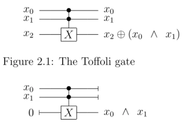
Figure 2.1: The Toffoli gate

x0 •

x1 •

0 _X _x₀ _∧ _x₁

Figure 2.2: Theand function (∧) embedded into the Toffoli gate

dauer’s principle [Lan00] which states that “any logically irreversible manipula-tion of informamanipula-tion, such as the erasure of a bit or the merging of two compu-tation paths, must be accompanied by a corresponding entropy increase in non-information bearing degrees of freedom of the non-information processing apparatus or its environment”. In practical terms, this means that reversible computation pro-vides us with a way of improving the energy efficiency of computers beyond the von Neumann-Landauer limit. This limit, given by the formulakT ln2, wherek is the Boltzmann constant and T is the temperature of the system, corresponds to the amount of energy that must be released per bit of lost information.

Any function can be thought of as reversible if it is of a one-to-one nature, but it is also possible to embed irreversible functions into a (larger) reversible func-tion. So that it isn’t the job of the programmer to ensure that the computations they produce are reversible, it is useful to look at a way of building up reversible computations from a small (universal) set of reversible functions, along with ways of combining these to build up arbitrary functions, which in themselves are re-versible, but may contain or define a function that is in itself irreversible. In the next section I shall introduce the notion of reversible circuits, and how they can be used to build up arbitrary reversible computations.

2.2.2 An introduction to reversible computation

Reversible computations in the sense that we are looking at here, can be thought of in terms of reversible circuits. The Toffoli gate (Figure 2.1) is an example of a

(25)

reversible circuit that is also universal. This means that any boolean function can be constructed purely from Toffoli gates, along with a notion of static inputs (input values set to a constant of either 0 or 1), and garbage (outputs that don’t form part of the required output of the boolean function, but that are required so that the computation is reversible). As an example, we can construct a reversible and

operation using only a single Toffoli gate, setting one of the inputs as a constant 0, and marking 2 of the outputs as garbage (Figure 2.2).

We shall talk more about constructing reversible (and embedding irreversible) computations in Chapter 3, and shall also introduce a category of reversible cir-cuits.

2.2.3 The relation between reversible and quantum

com-putation

Reversible computation is a good starting point to looking at Quantum compu-tation as all Quantum compucompu-tations are inherently unitary, and therefore of a reversible nature. In fact, as we’ll see later in this thesis, the operations available in reversible computation form a subset of the operations available in quantum computation. A result of this relationship is that we are also able to use the classical analogue throughout this thesis to help introduce ideas that can then be extended into the quantum realm.

2.3 An overview of quantum computation

There are many excellent introductory texts on quantum computation, such as [NC00], and other on-line resources such as [Pre04]. In this section, I shall give an overview of the subject. I aim to introduce the concepts in such a way as to complement the rest of this thesis, introducing the topics of qubits, superposition, entanglement, unitary operators and measurement in a similar way as they are used in the Quantum IO monad later (in Chapter 5).

(26)

2.3.1 Qubits

Qubits form the basis of quantum computation, and are the quantum counterpart to bits in classical computation. In fact as computer scientists when we look at qubits we often refer to them as having the base states|0i and |1i corresponding to the two states a classical bit can be in (0 or 1). We’ll see later that it is possible to use any orthogonal states as the basis for qubits, but the computational basis of _|0_i and _|1_i seems the most natural from a computational perspective. The ket

notation (_{| i}) was first devised by Dirac [Dir82], and is now extensively used in quantum mechanics, along with its dual (the bra, _{h |}), for describing quantum states. I shall explain a little more about the use of Dirac notation as we go on.

The main difference between qubits and classical bits is their ability to be in more than one of the base states at the same time, forming what is known as a superposition of states. The next section shall give more details about these superpositions, and go on to define what it is for a superposition to exist of more than a single qubit. Although we shall be describing qubits in terms of the states they can represent, we can also think of qubits in terms of a physical object that has the corresponding quantum mechanical properties, and as such, even qubits in an entangled state can be thought of as physically separated objects.

2.3.2 Superposition

When a qubit is in a superposition of states, it can be thought of as being in both states at the same time. However, there are some restrictions on what superpo-sitions a qubit can be in, which are inherent in the quantum mechanical aspects of their definition. Firstly, each base state that the super-position consists of has a corresponding complex amplitude (inC_{), and we are restricted by the fact that}

the sum of the squares of the absolute values of these amplitudes must be equal to one. So a qubit in an arbitrary super-position (_|ψ_i) can be thought of as being in the state|ψi=α|0i+β|1iwith the restriction that|α|2

+|β|2

= 1 (andα, β ∈C_).

(27)

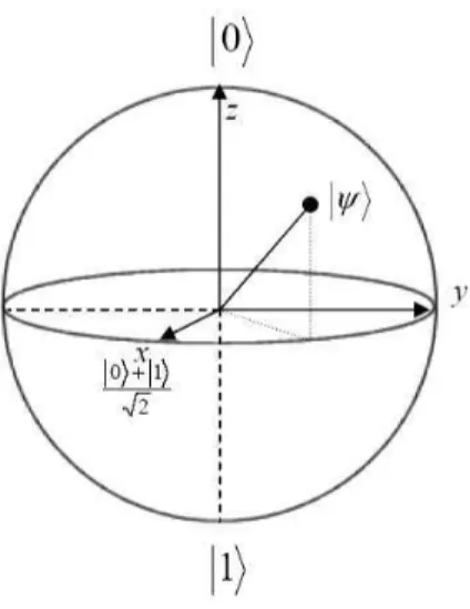
Figure 2.3: The Bloch sphere

lying on the surface of a unit sphere, commonly referred to as the Bloch sphere. Such a representation is able to occur because global phase doesn’t affect physical state, and any single qubit state can be rewritten such that the amplitude of the

|0i base state is real and non-negative. With a single qubit state reformulated in this way, we are able to write it in terms of two angles that represent a point on the unit sphere. That is, we have _|ψ_i=cosθ

2|0i+e

iφ_sinθ

2|1i, with 06θ 6π, and

0 6 φ < 2π. Figure 2.3 shows a representation of the Bloch sphere showing the single qubit states _|0_i, _|1_i, |0i√+|1i

2 and an arbitrary single qubit state |ψi. As an

aside, it is interesting to note that any two points that are opposite each other on the Bloch sphere are by definition orthogonal states, and as we mentioned earlier can be used as the basis for the state of a qubit.

The second, and main restriction that arises from quantum mechanics is the fact that it is impossible to know which current state an arbitrary qubit is in. For us to gain any knowledge of the state we must observe or measure the qubit. In doing so, the quantum mechanical aspects of the qubit are lost, and it will have collapsed into one of the original base states (_|0_i or_|1_i). All is not lost however, and the next section shall go over the details of these measurements, and what information we can actually gain from them.

(28)

2.3.3 Measurement

As we have just seen, measurements on qubits will collapse those qubits into one of their original base states. It is possible to measure a qubit in any orthogonal basis, but we shall once again stick to the computational basis in our examples. We are however able to gain some information about the original super-position of the measured qubit as the probabilities of measuring either base state are determined exactly by their corresponding amplitudes in the original super-position. In fact, the probability of measuring a certain base state is the absolute value squared of the corresponding complex amplitude. If we look at our examples from the Bloch sphere, we can see how this might work in practice. The states |0i, and |1i are quite boring as they always measure to their own value, but if we now look at the state |0i√+|1i

2 , which can also be written as 1

√

2|0i+ 1

√

2|1i, we can see that both

states have the same amplitude (of 1

√

2), which gives a corresponding probability of 1

2 for measuring either of the computational base states. This state is said to be in

an equal super-position of both the base states. More generally, for the arbitrary state_|ψ_i=α_|0_i+β_|1_iwe have that the probability of measuring _|0_ias_|α_|2_{, and}

the probability of measuring |1i as|β|2

.

As an aside, another interesting view of measurement was presented in [Eve57]. From hisRelative State view of quantum mechanics, measurement can be thought of as a process that splits the universe intoparallel universes, with each measure-ment outcome occurring in one of the parallel universes. As such, the reason we only see one outcome from a measurement is because we, as the observer, only continue to exist in the universe in which the corresponding measured state exists. This is slightly beyond the scope of this thesis, but is mentioned as it is one of the views that first interested me about the field of quantum computation.

So far, we have only been looking at the case of a single qubit, the next section shall go on to explain how a quantum system containing multiple qubits can behave, and shall go into detail as to how and what it means for qubits to become entangled.

(29)

2.3.4 Entanglement

Entanglement is a special form of superposition over a multiple qubit state. As such, it is useful to first look at arbitrary multiple qubit states. If we look at what happens in our classical analogue when we have multiple bits, we’ll notice that a system containing n bits can be in any of 2n _{base states, namely any of} the bit strings of length n. In fact, if we move back into the quantum realm, a system of n qubits can be in an arbitrary super-position over any of these bit strings of length n. That is, the state of an n qubit system can be defined by the sum over all the complex amplitudes of each of the 2n _{bit strings. We have a} similar restriction as for the single qubit case that the sum of the squares of the absolute values of all the complex amplitudes must be equal to 1. For example, the state of an arbitrary three-qubit system can be defined exactly by the sum

|ψ_i = α_|000_i+β_|001_i+γ_|010_i+δ_|011_i+ǫ_|100_i+ζ_|101_i+η_|110_i+θ_|111_i, with the restriction that_|α_|2₊

|β_|2₊ |γ_|2₊ |δ_|2₊ |ǫ_|2₊ |ζ_|2₊ |η_|2₊ |θ_|2 _{= 1. (again} with α, β, γ, δ, ǫ, ζ, η, θ _∈C₎

This exponential growth in the size of the available state space starts to hint at what gives quantum computers their increase in power over classical computers, but we have to keep in mind how these quantum states behave upon measurement. As we have previously seen, a single qubit will collapse into one of its base states upon measurement, and this behaviour generalises to multiple-qubit states. Upon measurement of all the qubits in a multiple qubit state, the whole system will be in one of the bit string base states, again with each base state having the probability of being measured equal to the square of the absolute value of its corresponding complex amplitude. However, it is also possible to only measure a subset of all the qubits in a multiple qubit state. Each time a qubit is measured, it will be in one of it’s base states (|0i or|1i), and in doing the measurement, every base state in the multiple-qubit super-position in which the qubit was in the opposite state is removed from the overall state of the system. That is, the measurement of a single qubit has a side-effect that can affect future measurements of other qubits

(30)

in the system. This dependency between qubits is known as entanglement. As an example we’ll look at some two qubit super-positions.

The state 1

2(|00i +|01i +|10i+ |11i) is in an equal super-position of two

qubits, that is, the probability of measuring any of the two-qubit base states is equal, namely 1

4. This is a valid two-qubit state, but is not an entangled state

as the measurement of either of the qubits doesn’t effect the state of the other qubit. The probability of measuring the first qubit as |0i is calculated by adding the probabilities of all the two-qubit base states in which the first qubit is a 0, namely _|00_i and _|01_i. Similarly, we can calculate the probability of measuring the first qubit as _|1_i by summing the probabilities of all the two-qubit states in which the first qubit is a 1, namely _|10_i and _|11_i. In each case here we get the probability of 1

2. Upon measurement, all the base-states which contain the first

qubit in the state it wasn’t measured in are removed from the overall state, and the amplitudes are re-normalised to reflect this. So, in this example, measuring a

|0i or a |1i leaves the rest of the system in the same state, namely 1

√

2(|0i+|1i),

meaning that our original state wasn’t an entangled state. It is also possible to see that our original state wasn’t an entangled state as we could have re-written it straight away as the tensor product ( 1

√

2(|0i+|1i))⊗( 1

√

2(|0i+|1i)). The tensor

product _⊗ is a useful operator to define the combination of quantum systems. In fact, in using | i notation it is used implicitly a lot of the time, with for example

|0i ⊗ |0i being given as simply |00i. If we now look at the two-qubit state 1

√

2(|00i+|11i), which is a bell state([Bel64])

and an example of a maximally entangled two-qubit state, we can see how entan-glement can effect measurements. This is a valid two-qubit state, as it is customary to leave out base states whose amplitudes are 0 when describing super-positions. In this example, if we were to measure the first qubit, we would as before work out the probabilities for measuring|0i or|1i by summing the probabilities for the corresponding two-qubit base states whose first qubit is in either state. Doing this, we again see a probability of 1

(31)

states. However, after measurement, when we look to see what state the rest of the system will be in, we’ll notice that there is only one state the second qubit can be in, namely exactly the same state as in which we have measured the first qubit. In other words, measuring the first qubit has had the side-effect of collapsing the second qubit into one of its base states.

It is this type of entanglement that lead to the EPR paradox [EPR35], which is often cited today as showing that quantum mechanics violates classical intuition. For example, classical intuition cannot explain the non-locality of measurements that is used when defining quantum teleportation. We shall look at quantum teleportation in some detail in section 2.6.7, and more information on the EPR paradox can be found in [Bel64] and [Mer85].

We have talked about quantum states, which can involve super-positions, and entanglement, but not really mentioned how these quantum states can be used for computation. We shall now introduce the concept of unitary transformations, and how they can be used to define quantum computations.

2.4 Unitary transformations

Unitary transformations describe the changes in state of the qubits involved in a computation. We have seen that we can define a quantum state of n qubits in terms of the complex amplitudes of the corresponding 2n _{bit strings of length} _n_. In fact, it is useful to be able to think of the state space of a quantum system in terms of the state spaces of the smaller systems it is comprised of. In quantum mechanical terminology, the state space of a single qubit is the two-dimensional Hilbert space, which we denoteH2. A Hilbert space is defined as a complex vector

space with an inner product, that is complete with respect to the inner product. Members of such a Hilbert space are defined by complex valued vectors of the same dimension as the Hilbert space, so the members of _H2, are complex valued

(32)

gives us Dirac’s bra-ket notation ([Dir82]) that we have already been using. That is, that the inner product of abra (_hψ_|) and aket (_|φ_i) can be given by thebra-ket

construction _hψ _|φ_i. |0i=    1 0   and |1i=    0 1   

More generally, from an arbitrary one qubit state_|ψ_i, we can derive

|ψ_i=α_|0_i+β_|1_i=α    1 0   +β    0 1   =    α 0   +    0 β   =    α β    We can now generalise this quantum mechanical view to quantum states of more than a single qubit. The state space of an n qubit system is the tensor product of the corresponding n two-dimensional Hilbert spaces. In other words, the state space of ann qubit system is the Hilbert space of dimension 2n_{, denoted} by H2n, and as such, members of this state space can be denoted by a complex

valued vector of dimension 2n _{whereby each element of the vector represents the} complex amplitude of the corresponding base state. For example, the two-qubit bell state we introduced in the measurement section can be given by

1 √ 2(|00i+|11i) = 1 √ 2          1 0 0 1         

If we were to use this terminology, unitary transforms for an n qubit system would relate to a unitary complex valued matrix of dimension 2n _× ₂n_{. That} is, a matrix that when multiplied by its conjugate transpose, gives the identity matrix. For a small number of qubits, this representation of unitary operators is quite straight forward, but the exponential growth in the dimensions of the matrix needed to represent a unitary means that for more than a few qubits this approach isn’t such a useful one. The next section looks at how we can look at unitary operators in terms of quantum gates, and circuits. These operators acting on a

(33)

small number of qubits, are often given in terms of their matrix representation, and the rules governing how circuits can be constructed from these gates are also defined in terms of the mathematical operations in the corresponding matrix representation. Chapter 3 goes on to look at a categorical model of these quantum gates and circuits.

2.5 The quantum gate model

The quantum gate model gives us a way of modelling unitary transformations over more than a few qubits in a simple way. Quantum circuits are defined by a universal set of quantum gates, and rules that govern how these gates can be combined. The gates themselves are usually given in terms of their corresponding matrix representation, and the combinators are given in terms of the underlying functions on matrices that they represent. There is more than one set of universal quantum gates, but the combinators usually boil down to parallel composition be-ing defined in terms of the tensor product of matrices, and sequential composition relating to matrix multiplication. In chapter 3, we present a categorical model of circuits, and our choice of quantum gates in this model leads on to the choice of unitary operators in our implementation of QIO (chapter 5). The quantum gate model also relates very nicely to the classical reversible circuits we used in section 2.2.

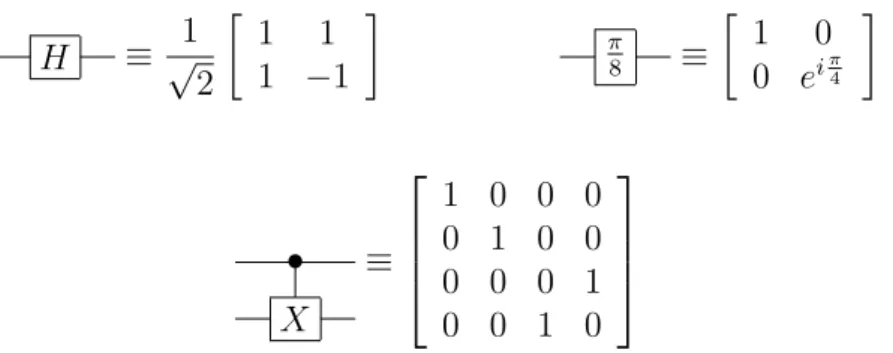
We now look at one specific example of a universal set of gates, although other universal sets of quantum gate do exist. We introduce here the universal family of gates introduced in [NC00], which also includes proofs of their universality (pages 188 to 198), in the sense that any unitary operator can be approximated up to an arbitrary accuracy. The family consists of theHadamard gate, the π₈ gate, and the

CNOT gate. Figure 2.4 gives the diagrams that we shall use to represent these gates, along with the corresponding matrix representations of the unitaries (We omit the phase gate here as it can be defined in terms of two π

(34)

H ≡ √1 2 1 1 1 ₋1 π 8 ≡ 1 0 0 eiπ 4 • X ≡     1 0 0 0 0 1 0 0 0 0 0 1 0 0 1 0    

Figure 2.4: A universal set of quantum gates, consisting of the Hadamard gate, the π

8 gate, and the CNOT gate.

Arbitrary unitary operations can now be defined as quantum circuits using these gates along with the operations of sequential composition and parallel com-position. Sequential composition joins circuits of the same arity (number of qubits) in sequence, and corresponds to matrix pre-multiplication of the first unitary by the second unitary. Parallel composition joins circuits so that they run in parallel over different qubits (giving rise to a circuit whose arity is the sum of the underly-ing arities). Parallel composition corresponds to the tensor product of the matrix representations.

As an example, we can use sequential composition to show that the Hadamard gate is its own inverse,

H H ≡ √1 2    1 1 1 ₋1   · √1 2    1 1 1 ₋1   ≡    1 0 0 1   ≡

Another example that uses both parallel and sequential composition is to show that following circuits are equivalent.

H • H H X H _ _ _ _ _ _ _ _ _ _ _ _ _ _ _ _ _ _ _ _ ≡ X •  _≡   1 0 0 0 0 0 0 1 0 0 1 0 0 1 0 0    

The groupings in the diagram represent the order in which we shall perform the steps of the matrix calculations (Although in practise the order in which we do the two matrix multiplications doesn’t matter as the operation is associative). The first step is to define the matrix representation of the unitary that performs

(35)

two Hadamard gates in parallel. H H _ _ _ _ ≡ √1 2    1 1 1 ₋1   ⊗ √1 2    1 1 1 ₋1   ≡ 1 2          1 1 1 1 1 ₋1 1 ₋1 1 1 ₋1 ₋1 1 −1 −1 1         

Next, we calculate the unitary that is obtained by running this in sequence with the CNOT gate.

H • H X _ _ _ _ _ _ _ _ _ _ _ _ _ _ _ _ ≡          1 0 0 0 0 1 0 0 0 0 0 1 0 0 1 0          ·1₂          1 1 1 1 1 −1 1 −1 1 1 −1 −1 1 ₋1 ₋1 1          ≡ 1₂          1 1 1 1 1 −1 1 −1 1 −1 −1 1 1 1 ₋1 ₋1         

Finally, we calculate the unitary that we obtain from running the previous unitary in sequence again with the two parallel Hadamard gates.

H • H H X H _ _ _ _ _ _ _ _ _ _ _ _ _ _ _ _ _ _ ≡ 1 2        1 1 1 1 1 ₋1 1 ₋1 1 1 ₋1 ₋1 1 ₋1 ₋1 1        ·1 2        1 1 1 1 1 ₋1 1 ₋1 1 ₋1 ₋1 1 1 1 ₋1 ₋1        ≡        1 0 0 0 0 0 0 1 0 0 1 0 0 1 0 0        Although we have given this universal family of circuits, in the rest of this section we shall use gates that represent arbitrary single qubit rotations, which are given along with their corresponding matrix representation. We also use controlled versions of larger unitaries, for ease of notation, although these too could be derived from this universal family of gates we have given above.

Having introduced the concept of quantum computation, we shall now go on to look at some famous quantum algorithms and how they use quantum states, along with entanglement to achieve classically infeasible tasks. In many cases, we also include the corresponding circuit diagram that represents the algorithm as a quantum computation.

(36)

2.6 Quantum Algorithms

2.6.1 Deutsch’s Algorithm

Deutsch’s algorithm [Deu85] is often used as an introduction to quantum algo-rithms as it is in essence the most simple algorithm to have been found that can be proved to give a result faster than the classical solution to the same problem. It involves being given an unknown function that takes a single boolean value as input, and returns a single boolean value as its output. You are then asked to find out whether the function you have been given is balanced or constant whilst only applying the function as few times as possible. Classically, it is easy to show that you must apply the function twice to get a certain result (once for each possible input value), but using Deutsch’s algorithm, it is possible to apply the function only once (albeit over a quantum state), and gain enough information from the result to determine the solution to the original problem. It is a simple algorithm to introduce first as it only uses two qubits, and as such is small enough so that we can go through all the mathematical detail without filling too much space.

• We start with the top qubit in the state _|0_i and the bottom qubit in state

|1i.

|0i H x x H

Uf

|1_i H y y_⊕f(x)

• After the First Hadamard gates we are left with the top qubit in the _|+_i state (_|0_i+_|1_i), and the bottom qubit in the state _|−i (_|0_{i − |}1_i).

|0i+|1i x x H

Uf

|0_{i − |}1_i y y_⊕f(x)

(37)

– f(x) = 0, has no overall effect on either qubit so we are left in the state (_|0_i+_|1_i)(_|0_{i − |}1_i) as before.

– f(x) = 1, adds 1 onto the value of the bottom qubit for both parts of the value of the top qubit, so we are left with the state (|0i+|1i)(|1i − |0i), which is equivalent to the state ₋(_|0_i+_|1_i)(_|0_{i − |}1_i).

– f(x) =x, adds 1 onto the value of the bottom qubit for the |1i part of the top qubit, so we are left with the state|0i(|0i−|1i) +|1i(|1i−|0i), which is equivalent to the state _|0_i(_|0_{i − |}1_i)_{− |}1_i(_|0_{i − |}1_i) and can be simplified to (_|0_{i − |}1_i)(_|0_{i − |}1_i).

– f(x) =¬x, adds 1 onto the value of the bottom qubit for the|0ipart of the top qubit, so we are left with the state|0i(|1i−|0i) +|1i(|0i−|1i), which is equivalent to the state _|0_i(_|1_{i − |}0_i)_{− |}1_i(_|1_{i − |}0_i) and can be simplified to (_|0_{i − |}1_i)(_|1_{i − |}0_i) or ₋(_|0_{i − |}1_i)(_|0_{i − |}1_i).

• We can see that for the constant cases (f(x) = 0 and f(x) = 1) we have the states_±(_|0_i+_|1_i)(_|0_{i − |}1_i), and for the balanced cases (f(x) = x and

f(x) = ¬x) we have the states±(|0i − |1i)(|0i − |1i). We can now apply the final Hadamard in both cases.

± |0_i+_|1_i H ± |0_i

|0_{i − |}1_i _|0_{i − |}1_i

± |0_{i − |}1_i H ± |1_i

|0_{i − |}1_i _|0_{i − |}1_i

• As global phase (the ±) is not observable under measurement, we can now measure the top qubit and ascertain exactly whether the original function was one of the balanced or one of the constant functions, measuring a_|1_ior a _|0_i respectively.

2.6.2 Deutsch-Jozsa Algorithm

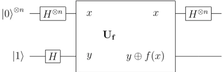
The Deutsch-Jozsa algorithm [DJ92] is an extension to, and generalisation of, Deutsch’s algorithm to determine whether a boolean function of an arbitrary num-ber of inputs, but still only one output, is balanced or constant (and it is guaran-teed to be one of these). For a given function which takesn input booleans, there

(38)

|0_i⊗n H⊗n _x _x _H⊗n

Uf

|1_i H y y_⊕f(x)

Figure 2.5: The Deutsch-Jozsa Algorithm

is now an input domain of size 2n_{, and classically it can be seen that in the worst} case the function will have to be applied to one more than half of these possible inputs (2n₋1

+ 1) to see if the function is balanced or constant. However, just as before for Deutsch’s algorithm, we can use the Deutsch-Josza algorithm to attain a solution having only had to apply the given function once (again, over a quantum state). The algorithm works in a very similar way to Deutsch’s algorithm, requir-ing one more qubit than the number of inputs to the boolean function. Figure 2.5 shows us the circuit for the Deutsch-Jozsa algorithm, where a measurement of the top n qubits after the application of the circuit will reveal whether the input function f was constant or balanced.

2.6.3 Simon’s Algorithm

Simon’s algorithm [Sim94] is another quantum algorithm that was shown to give a solution faster than the best possible classical solution. It gives the solution to a very specific (somewhat contrived) problem, in a time exponentially faster than the best known classical solution. We mention it briefly here as it is often cited as the inspiration behind Shor’s factorisation algorithm which we look at below.

The problem involves being given a function f : 0,1n

→ 0,1m _with _m _> _n_. The function is guaranteed to be either one-to one, or there exists a bit string of length n (s), such that for any pair of different inputs to the function (x,y),

f(x) = f(y) if and only if x⊕s = y (and y = x⊕s). Simon’s algorithm is then able to determine which of the cases the function falls into, and in the second case is able to return the value ofs. Simon described this algorithm as being a solution to the problem Is a function invariant under some xor-mask?.

(39)

2.6.4 Grover’s Algorithm

Grover’s algorithm [Gro96], otherwise known as Grover’s database search algo-rithm, was discovered by Lov Grover in 1996. It is a quantum algorithm for searching an unsorted database. It gives a quadratic speed-up over the fastest classical solution, which is a linear search. For a database of size N, we must encode a quantum state over N distinct base-states, and define a unitary that is able to add a negative phase only to the base state that represents the element we are searching for. Grover showed that such a unitary is able to be defined, and used in a probabilistic quantum algorithm to return the state being searched for.

2.6.5 Quantum Fourier Transform

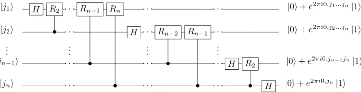
Although not necessarily thought of as a quantum algorithm in its own right, the quantum Fourier transform is used in many other quantum algorithms to extract certain information we want from a quantum super-position of states. More precisely, the quantum Fourier transform is used to increase the amplitudes of certain states in a super-position that represent the states that are “useful” for gaining the result of certain quantum algorithms. This is a very over-simplified view of what the quantum Fourier transform does, but this view of it is the basis for how Shor defined his factorisation algorithm. His algorithm uses the quantum Fourier transform to extract the period of a modular exponentiation function, from a super-position of the results of the modular exponentiation function applied to an equal superposition of its possible input states. The quantum Fourier transform can basically be thought of as the fast discrete Fourier transform applied to a quantum register. The discrete Fourier transform can be thought of as mapping functions in the time domain into functions in the frequency domain. In other words, decomposing a function into a series of sinusoidal functions of different frequencies. An excellent derivation of the quantum Fourier transform is given in [NC00] on pages 216 to 221. The circuit they derive is given here in figure 2.6 for reference.

(40)

Figure 2.6: A circuit for the Quantum Fourier transform, where Rk is given by the unitary 1 0 0 e22πik

2.6.6 Shor’s Algorithm

Shor’s algorithm is possibly the most famous of all the quantum algorithms as it provides an exponential speed up over the fastest known classical solution to what is thought to be a classically infeasible operation (requiring a process that runs for an exponential amount of time compared to the input). Shor showed [Sho94] that finding the prime factors of a large integer could be restated as the problem of finding the period of a specifically constructed modular exponentia-tion funcexponentia-tion, and he went on to give a quantum algorithm that could solve this task in polynomial time. This polynomial time solution does however require a suitably sized quantum computer with enough qubits to encode both the input and output integers, which is many more than the handful available in current implementations (such as [VSB+

01]).

Shor’s algorithm is sometimes referred to as the “Killer Application” for quan-tum computers. This nomenclature came about because factorising large numbers was thought to be so computationally infeasible that it forms the basis of the RSA encryption protocol ([RSA77]). The RSA encryption protocol is a very widely used public-key protocol for sending secure information over public channels such as the Internet. It works on the principle that multiplying 2 large prime numbers (p and

q) is computationally easy, and a public and private key can be computed from the result (n=p∗q). However, if it is possible for an eavesdropper to computep

Towards a formally verified functional quantum programming language

Green, Alexander S. (2010) Towards a formally verified

functional quantum programming language. PhD thesis,

University of Nottingham.

Towards a formally verified functional quantum

programming language

Alexander S. Green, BSc.

Acknowledgements

Contents

List of Figures

Chapter 1

Introduction

1.1

Introduction

1.2

Background

1.2.1

Related Work

1.3

Overview of thesis

1.4

Joint Work

Chapter 2

Quantum Computation

2.1

The history of quantum computation

2.2

Reversible Computation

2.2.1

The history of reversible computation

2.2.2

An introduction to reversible computation

2.2.3

The relation between reversible and quantum

com-putation

2.3

An overview of quantum computation

2.3.1

Qubits

2.3.2

Superposition

2.3.3

Measurement

2.3.4

Entanglement

2.4

Unitary transformations

2.5

The quantum gate model

2.6

Quantum Algorithms

2.6.1

Deutsch’s Algorithm

2.6.2

Deutsch-Jozsa Algorithm

2.6.3

Simon’s Algorithm

2.6.4

Grover’s Algorithm

2.6.5

Quantum Fourier Transform

2.6.6

Shor’s Algorithm