Early
bird
Computer Science•21(3) 2020 https://doi.org/10.7494/csci.2020.21.3.3824
Grzegorz Gurgul, Marcin Lo´
s, Maciej Paszy´
nski
Victor Calo
LINEAR COMPUTATIONAL COST IMPLICIT
SOLVER FOR PARABOLIC PROBLEMS
Abstract In this paper, we use the alternating direction method for isogeometric finite elements to simulate transient problems. Namely, we focus on a parabolic problem and use B-spline basis functions in space and an implicit time-marching method to fully discretize the problem. We introduce intermediate time-steps and separate our differential operator into a summation of the blocks that act along a particular coordinate axis in the intermediate time-steps. We show that the resulting stiffness matrix can be represented as a multiplication of two (in 2D) or three (in 3D) multi-diagonal matrices, each one with B-spline basis functions along the particular axis of the spatial system of coordinates. As a result of these algebraic transformations, we get a system of linear equations that can be factorized in a linearO(N)computational cost at every time-step of the implicit method. We use our method to simulate the heat transfer problem. We demonstrate theoretically and verify numerically that our implicit method is unconditionally stable for heat transfer problems (i.e., parabolic). We conclude our presentation with a discussion on the limitations of the method.
Keywords isogeometric analysis, implicit dynamics, linear computational cost, direct solvers
Citation Computer Science 21(3) 2020: 323–339
Copyright ©2020 Author(s). This is an open access publication, which can be used, distributed and reproduced in any medium according to the Creative Commons CC-BY 4.0 License.
Early
bird
1. Introduction
The alternating directions implicit method (ADI) was first introduced in [4, 11, 28, 30] to deal with finite-difference simulations for time-dependent problems. The method is currently used as a solution for a wide class of problems [18, 19]. In the ADI method for finite-difference simulations, the partial differential equations (PDE) are first discretized in space using spatial stencil and then in time using intermediate time-steps. For example, let us consider the heat equation in two dimensions:
du
dt −∆u=f, (1)
with either Dirichlet or Neumann boundary conditions. We now discretize it using central differences with respect to the xandy directions:
du dt − ∂2u ∂x2 − ∂2u ∂y2 =f , (2) du dt − ui−1,j−2ui,j+ui+1,j h2 −
ui,j−1−2ui,j+ui,j+1
h2 =f, (3)
and the ADS method introduces an intermediate time step:
uti,j+0.5−ut i,j τ /2 −
uit−+01.,j5−2ui,jt+0.5+uti+1+0.,j5
h2 =
uti,j−1−2uti,j+uti,j+1
h2 +f
t, uti,j+1−uti,j+0.5
τ /2 −
ui,jt+1−1−2ui,jt+1+uti,j+1+1
h2 =
uit−+01.,j5−2ui,jt+0.5+uti+1+0,j.5
h2 +f
t+0.5,
(4) where τ is the time-step size, andft, ft+0.5 denote the forcing term in time-step t
and in the middle between steps tandt+ 1, respectively. The resulting two systems of linear equations are tridiagonal and can be solved with a linear computational cost. In this paper, we apply the above approach to simulations using isogeometric analysis (IGA) [1,8]. The main idea of IGA is to apply B-splines or NURBS [29] basis functions in finite element simulations. It has multiple applications in time-dependent simulations, including phase-field models [9, 10], phase-separation simulations with an application to cancer growth simulations [16, 17], wind turbine aerodynamics [23], incompressible hyper-elasticity [12], turbulent flow simulations [6], the transport of drugs in cardiovascular applications [22], or blood flow simulations and drug transport in artery simulations [3, 5].
An alternating direction solver (ADS) is a fast linear solver that exploits the Kronecker product structure of the matrix that arises in some finite element simu-lations. It was recently applied [13–15] for a fast solution for the isogeometric L2
orthogonal projection onto the finite element space of B-splines. There, the authors solved a projection problem discretized with a tensor product basis comprised of basis functions of the following form:
Bi1,...,id(x1, . . . , xd) =B
x1
i1(x1)· · ·B xd
Early
bird
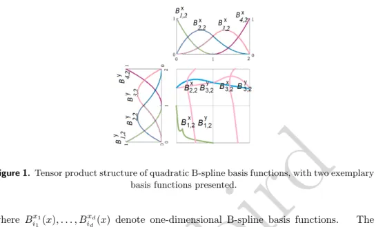
Figure 1. Tensor product structure of quadratic B-spline basis functions, with two exemplary basis functions presented.
where Bx1
i1(x), . . . , B xd
id(x) denote one-dimensional B-spline basis functions. The
direction-splitting schemes deliver a fast inversion method for the spatial discretization that is obtained by grouping the one-dimensional B-splines together along particular spatial axes, assuming that the basis functions have a tensor product structure (as Figure 1 sketches). In this case, we can index tensor product basis functions using pairs (in 2D) of indices of one-dimensional basis functions; e.g.,
Bi,j(x, y) =Bix(x)B y
j(y). (6)
For the purpose of visualizing the matrices and vectors in space that are spanned by this basis, such double indices can be linearized by ordering them lexicographically. The Gram (mass) matrix of B-spline basis on 2D domain Ω = Ωx×Ωycan be expressed
as follows: M(i,j)(k,l)= (Bi,j, Bk,l) = Z Ω Bi,jBk,ldΩ = Z Ω Bxi(x)Bjy(y)Bkx(x)Bly(y) dΩ = Z Ω (BiBk)(x) (BjBl)(y) dΩ = Z Ωx BiBkdx Z Ωy BjBldy ! =MxikM y jl, (7)
where (·,·) = (·,·)L2(Ω). In other words, Gram matrixM=Mx⊗Myis the Kronecker
product of two multi-diagonal matrices with the corresponding structure of a mass matrix build from one-dimensional B-spline basis functions. Such a matrix can be factorized in a linear computational cost (see Appendix B).
This idea can be directly applied to speed up simulations using explicit time dis-cretizations, since the simulation of dynamics using the explicit time-stepping scheme can be expressed as a sequence of isogeometricL2projections in the following manner. Given a time-dependent problem with spatial operator L and Dirichlet or Neumann
Early
bird
boundary conditions
du
dt −Lu=f , (8)
we discretize time using the explicit Euler scheme and obtain
ut+1=ut+τ Lut+τ f , (9)
where τ is the time-step size. Then, we pass to the weak formulation by multiplying the above equation by test functionv, which leads to
(ut+1, v) = (ut+τ Lut+τ f, v), (10)
where ut+1 =Pi,ja t+1
i,j Bix;p(x)B y
j;q(y) and ut =Pi,jati,jBix;p(x)B y
j;q(y). Thus, each
time-step is equivalent to computing an orthogonal L2 projection of the right-hand side of Eq. (9), which can be done in linear computational cost with respect to the number of degrees of freedom in the system.
The method was used for performing fast simulations of dynamics with explicit time discretization [20, 24–26, 31, 32], since the explicit time integration scheme with isogeometric discretization is equivalent to the sequence of isogeometricL2orthogonal
projections, which can be solved using the direction splitting of the later kind. In this paper, we extend this methodology to dynamics simulations with im-plicit time discretization by collecting different terms as a sequence of multi-diagonal inversions.
The structure of the paper is as follows. In Section 2, we start from a description of the direction splitting for the Laplace operator. Next, in Section 3, we present the numerical results for the two-dimensional model heat transfer problem. Section 4 derives the proof of unconditional stability for our direction-splitting method. We conclude the paper in Section 5. We provide two appendices with some Lemmas used for proving the unconditional stability of the scheme and with the general description of the alternating directions solver.
2. Direction splitting for Laplace operator
We express this parabolic system as a sequence of implicit time-steps, which is
du
dt −Lu=f , (11)
where, for the sake of simplifying the discussion, we assume that the coefficients are constant, the domain is the unit is square, and the differential operator is separable; that is,L=Lx+LywhereLαcontains spatial derivatives only with respect toα(e.g.,,
Laplacian, whereL=Lx+Ly =∂ 2u ∂x2 +
∂2u
∂y2). Furthermore, we impose either uniform
Dirichlet or zero Neumann boundary conditions. Thus, to apply the alternating direction implicit scheme, we introduce a sequence of intermediate time-steps, which is
ut+0.5−ut
Early
bird
ut+1−ut+0.5τ /2 −Lxut+0.5−Lyut+1=ft+0.5. (13) We rewrite these equations by collecting the known variables on the right-hand side as follows: ut+0.5− τ 2Lxut+0.5=ut+ τ 2Lyut+ τ 2ft, ut+1− τ 2Lyut+1=ut+0.5+ τ 2Lxut+0.5+ τ 2ft+0.5. (14) Now, we transform the problem into a weak form multiplying by test functions and applying integration by parts to get the following weak forms:
(v, ut+0.5) + τ 2 ∂v ∂x, ∂ut+0.5 ∂x = (v, ut)− τ 2 ∂v ∂y, ∂ut ∂y +τ 2(v, ft), (15) (v, ut+1) + τ 2 ∂v ∂y, ∂ut+1 ∂y = (v, ut+0.5)− τ 2 ∂v ∂x, ∂ut+0.5 ∂x +τ 2(v, ft+0.5), (16) where the resulting boundary terms vanish due to the boundary conditions.
In the sequel, we limit the discussion to the first of the above equations; the other can be treated in a similar fashion.
Definition 1. Let VN
x be the space of functionsf ∈L2(Ω) such that distributional derivative ∂f /∂x is a regular distribution and∂f /∂x∈L2(Ω), which is
VxN = v∈L2(Ω) : ∂v ∂x ∈L 2(Ω) , (17) and letVD
x be its subspace of functions vanishing on the boundary:
VxD=VxN∩H01(Ω). (18)
If we consider a problem with Neumann boundary conditions, letVx=VxN; otherwise, Vx=VxD. Space Vy can be defined analogously.
We end up with the following variational problem: Givenw∈H2(Ω), findu∈V x such as b(v, u) =l(v) ∀v∈Vx, b(v, u) = (v, u) +τ 2 ∂v ∂x, ∂u ∂x , l(v) = (v, w) +τ 2 v,∂ 2w ∂y2 +τ 2(v, f). (19) We have integrated the right-hand-side term back by parts to keep the continuity of the linear form. This is necessary since, due to the definition of Vx, test function v
is not required to possess a weak derivative in the y direction. The assumption that
Early
bird
Definition 2. Let τ >0. Foru, v∈Vx, let
(v, u)Vx = (v, u) + τ 2 ∂v ∂x, ∂u ∂x . (20)
It is a scalar product that induces the following norm:
kuk2V x=kuk 2 L2+ τ 2 ∂u ∂x 2 L2 . (21)
Lemma 1. SpaceVx with normk·kVx is a Hilbert space.
Proof. Let {un} be a Cauchy sequence in Vx. By the definition of the norm of Vx,
{un} and {∂un/∂x} are Cauchy sequences in L2(Ω); so, by its completeness, there
exist L2 functions u,ux such that un →uand∂un/∂x→ux in the sense of theL2
norm. Letφ∈D(Ω) be a test function in the sense of the theory of distributions. We have u,∂φ ∂x = lim n→∞ un, ∂φ ∂x =− lim n→∞ ∂u n ∂x , φ =−(ux, φ) sinceφ∈L2(Ω), sou
xis a distributional derivative ofuand, thus,u∈Vx. Therefore, Vx is complete.
Theorem 1. Bilinear form
b(v, u) = (v, u) +τ 2 ∂v ∂x, ∂u ∂x (22) defined on Vx is coercive. Proof. We have b(u, u) =kuk2L2+ τ 2 ∂u ∂x 2 L2 =kuk2V x. (23)
Theorem 2. Abstract variational problem: for a given continuous linear func-tional l∈Vx0, find u∈Vx such that
b(u, v) =l(v) ∀v∈Vx (24) is well-posed.
Proof. Bilinear formbis obviously continuous and is coercive due to Theorem 1. By the Lax-Milgram theorem, the variational problem is well-posed.
Early
bird
We discretize the above abstract variational problem using a finite element space Vh ⊂ Vx comprised of linear combinations of the tensor product of B-spline
basis functions of order p, which is
Vh= span{Ni,j}i,j Ni,j(x, y) =Bix(x)B y
j(y), (25)
whereBx i andB
y
j are basis B-spline functions in thexandy directions, respectively.
Let us first focus on System (15). We approximate ut+0.5 =
P k,la t+0.5 k,l B x k(x)B y
l(y) and test with v = B x i(x)B
y
j(y). Our previous sub-step
so-lution is also given as linear combination ut=Pk,latk,lBkx(x)B y l(y). X k,l atk,l+0.5 " Bkx(x)Bly(y), Bix(x)Bjy(y)+τ 2 ∂(Bx k(x)B y l(y)) ∂x , ∂(Bxi(x)Bjy(y)) ∂x !# = X k,l atk,l " Bkx(x)Bly(y), Bix(x)Bjy(y) −τ 2 ∂(Bx k(x)B y l(y)) ∂y , ∂(Bx i(x)B y j(y)) ∂y !# + τ 2(ft, B x i(x)B y j(y)).
Using the fact that ∂Bxk(x)
∂y = ∂Byk(y) ∂x = 0, we obtain X k,l atk,l+0.5 Bkx(x)Bly(y), Bxi(x)Bjy(y) +τ 2 ∂Bx k(x) ∂x B y l(y), ∂Bx i(x) ∂x B y j(y) = X k,l atk,l " Bkx(x)Bly(y), Bix(x)Bjy(y)−τ 2 B x k(x) ∂Bly(y) ∂y , B x i(x) ∂Bjy(y) ∂y !# + τ 2(ft, B x i(x)B y j(y)).
We can separate the directions and use the fact that theyterms are identical, which can be expressed as a Kronecker product:
X k,l atk,l+0.5 (Bkx(x), Bxi(x)) +τ 2 ∂Bx k(x) ∂x , ∂Bx i(x) ∂x Bly(y), Bjy(y) = X k,l atk,l " Bkx(x)B y l(y), B x i(x)B y j(y) −τ 2 B x k(x) ∂Bly(y) ∂y , B x i(x) ∂Byj(y) ∂y !# + τ 2(ft, B x i(x)B y j(y)).
Early
bird
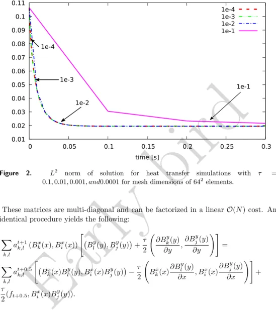
0.01 0.02 0.03 0.04 0.05 0.06 0.07 0.08 0.09 0.1 0.11 0 0.05 0.1 0.15 0.2 0.25 0.3 time [s] 1e-4 1e-3 1e-2 1e-1 1e-4 1e-1 1e-2 1e-3Figure 2. L2 norm of solution for heat transfer simulations with τ = 0.1,0.01,0.001, and0.0001 for mesh dimensions of 642 elements.
These matrices are multi-diagonal and can be factorized in a linearO(N) cost. An identical procedure yields the following:
X k,l atk,l+1(Bkx(x), Bxi(x)) " Bly(y), Byj(y)+τ 2 ∂Bky(y) ∂y , ∂Bjy(y) ∂y !# = X k,l atk,l+0.5 " Bkx(x)Bly(y), Bxi(x)Bjy(y) −τ 2 B x k(x) ∂Byl(y) ∂x , B x i(x) ∂Bjy(y) ∂x !# + τ 2(ft+0.5, B x i(x)B y j(y)).
Thus, we obtain an alternating direction implicit IGA discretization with a solu-tion cost ofO(N).
3. Numerical results for Laplace operator
We test the alternating direction implicit solver that we propose for the heat transfer problem with zero forcing over a two-dimensional mesh of 64×64 elements using quadratic B-spline basis functions. The initial state is a ball of heat concentrated in
Early
bird
the center of the domain given by
u(x,0) =φ(min{1,12kx−(0.5,0.5)k2}), (26)
φ(s) = (1−s)2(1 +s)2, (27) and we employ zero Neumann boundary conditions. Due to the boundary conditions and zero forcing, the steady state solution is a constant function with a value equal to the average of the initial state; i.e.,
lim t→∞u(·, t) = 1 |Ω| Z Ω u(x,0)dx= 1 45 ≈0.02. (28) We use time-step sizes of 10−1, 10−2, 10−3, and 10−4. We plot theL2 norm of
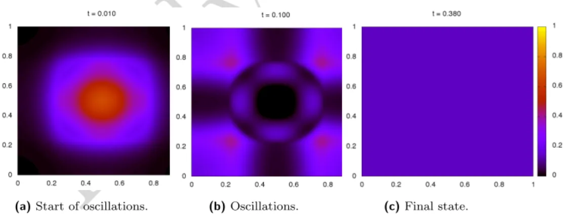
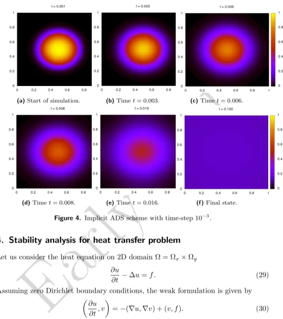
the solution in Figure 2. From the plots, we can conclude that the solutions always converge to the same final solution even if it is oscillating at the beginning for large time-step sizes (like for 10−1). This is illustrated in Figure 3, where we employ the largest time-step (10−1). Although the quality of the intermediate solutions is very poor for such a large time-step (as expected), the equilibrium solution is ultimately approximated fairly well. We will prove the asymptotic stability of the scheme; thus, the transient local growth of the solution is not discarded. However, these local phenomena disappear as time progresses. Snapshots from the simulation with a time-step size of 10−4 without any oscillations are presented in Figure 4. These numerical results are obtained for a time-step size of 10−3.
(a)Start of oscillations. (b)Oscillations. (c)Final state.
Figure 3. Implicit ADS scheme with time-step 10−1.
Alternative approach for direction splitting is discussed in paper [34], where we focus on hyperbolic wave propagation problems; however, the problem matrix is ap-proximated as a Kronecker product of (Mx+αSx)⊗(My+αSY) (with mass and
stiffness matrices) where the higher-order terms with respect toαare neglected. This method also results in an unconditionally stable scheme and a linear computational cost solver. However, the method presented in this paper does not approximate the matrix – it proposes the splitting of the whole system.
Early
bird
(a)Start of simulation. (b)Timet= 0.003. (c)Timet= 0.006.(d)Timet= 0.008. (e)Timet= 0.016. (f)Final state.
Figure 4. Implicit ADS scheme with time-step 10−3.
4. Stability analysis for heat transfer problem
Let us consider the heat equation on 2D domain Ω = Ωx×Ωy ∂u
∂t −∆u=f . (29)
Assuming zero Dirichlet boundary conditions, the weak formulation is given by
∂u ∂t, v =−(∇u,∇v) + (v, f). (30) LetBij(x, y) =Bxi(x)B y
j(y) be the standard tensor product basis. We seek a solution
of form
u(x, t) =Xuij(t)Bij(x).
We will analyze the spectral radius of the step operator for both the explicit Euler method and our implicit method. The method is stable when the spectral radius is less than 1 [21].
Let us denote
M=
Early
bird
and Mx= (Bix,B x k)L2(Ω x) Kx= (∂xBxi, ∂xBxk)L2(Ω x) , (32)and similarly for My, Ky. These matrices are symmetric and positive definite as
Gram matrices of certain sets of linearly independent functions. Under the simple geometrical mapping, we assume that we can express the first two equations of (31) in terms of (32) as
M=Mx⊗My K=Kx⊗My+Mx⊗Ky. (33)
For simplicity, let us consider the case where forcing termf is time-independent, and we can assume f = 0. In the implicit scheme, we have
un+1 2, v +τ 2 ∂u n+1 2 ∂x , ∂v ∂x = (un, v)− τ 2 ∂un ∂y , ∂v ∂y , (un+1, v) + τ 2 ∂u n+1 ∂y , ∂v ∂y =un+1 2, v −τ 2 ∂u n+1 2 ∂x , ∂v ∂x , (34) which results in the following algebraic relationships:
M+τ 2Kx⊗My un+1 2 = M−τ 2Mx⊗Ky un, M+τ 2Mx⊗Ky un+1= M−τ 2Kx⊗My un+1 2. (35) SinceM=Mx⊗My, h Mx+ τ 2Kx ⊗My i un+1 2 = h Mx⊗ My− τ 2Ky i un, h Mx⊗ My+ τ 2Ky i un+1= h Mx− τ 2Kx ⊗My i un+1 2. (36) Let us denote S+x =Mx+ τ 2Kx S − x =Mx− τ 2Kx S+y =My+ τ 2Ky S − y =My− τ 2Ky. (37) Then, we can write
S+x ⊗My un+1 2 = Mx⊗S−y un, Mx⊗S+y un+1=S−x ⊗Myun+1 2. (38) We can finally combine the two steps:
un+1=Mx⊗S+y −1 S−x ⊗My S+x ⊗My −1 Mx⊗S−y un, (39)
which can be simplified by using the properties of the Kronecker product:
Early
bird
•(A⊗B) (C⊗D) = (AC)⊗(BD) whenever the products make sense. Using these, we conclude that
Mx⊗S+y −1 S−x ⊗My S+x ⊗My −1 Mx⊗S−y = h M−x1⊗ S+y−1i S−x ⊗My h S+x−1 ⊗M−y1i Mx⊗S−y = h M−x1⊗ S+y−1i h S−x S+x−1 ⊗Ii Mx⊗S−y = h M−x1⊗ S+y−1i h S−x S+x−1 Mx⊗S−y i = h M−x1S−x S+x−1 Mx i ⊗h S+y−1 S−yi. (40) Since the eigenvalues ofA⊗Bare products of eigenvalues ofAandB, we only seek to determine the eigenvalues of the above two matrices. The first matrix is similar to S−x(S+x)
−1
and, thus, has the same eigenvalues. Furthermore, AB and BA al-ways have the same spectrum, soS−
x(S+x)
−1
has the same eigenvalues as (S+ x)
−1
S−
x.
By Lemma 3 (see Appendix A), the eigenvaluesλof (S+ x) −1 S− x and S+y −1 S− y
sat-isfy |λ|<1, so the full matrix of the single step has a spectral radius of less than 1. Thus, the implicit ADS scheme is unconditionally stable.
5. Conclusion
In this paper, we introduce mixed space-time discretizations based on the alternating direction method for isogeometric discretizations. We introduce intermediate time-steps to use the Kronecker product structure to invert in linear cost of a sequence of semi-implicit discretizations over time. The resulting isogeometric implicit alternating direction method is unconditionally stable for the heat transfer problem in 2D with an arbitrary time-step size. This was verified theoretically and numerically.
Extending the presented method to a more general context poses some challenges. The Kronecker product structure of the matrix required by the alternating directions solver imposes some rather considerable restrictions on the geometry of the domain as well as the problems themselves. Although it is possible to extend our approach to domains that can be parameterized in such a way that the Jacobian of the map is a product of univariate functions, applying it on arbitrarily complicated domains remains an open problem. For similar reasons, the arbitrary variable diffusivity coef-ficient in the heat equation can break the Kronecker product structure. Nevertheless, the proposed method (when applicable) can greatly decrease computational costs while retaining good stability properties.
Acknowledgments
This work is supported by National Science Center, Poland – Grant No. 2017/26/M/ ST1/ 00281.
Early
bird
A. Lemmas
Lemma 2. Let A, B be symmetric and positive-semidefinite. Then, AB has non-negative eigenvalues.
Proof. Exercise 7.2.P21 in [33].
Lemma 3. Let A, B be symmetric and positive-definite. For each eigenvalue λ of (A+B)−1(A−B), we have|λ|<1.
Proof. Letλ6= 0 be such an eigenvalue, and letx be the corresponding eigenvector. Then,
(A+B)−1(A−B)x=λx, (41) and so
(A−B)x=λ(A+B)x,
(1−λ)Ax= (1 +λ)Bx. (42)
Since B is positive-definite, then it is nonsingular; thus, Bx 6= 0. Thus, λ 6= 1. Multiplying by xTon the left gives
xTAx=1 +λ 1−λ x
TBx. (43)
SinceAandB are positive definite, both products are positive; thus,λ∈Rand
1 +λ
1−λ>0 =⇒λ
2<1 ⇐⇒ |λ|<1. (44)
B. Linear computational cost solver
Gram matrixM=Mx⊗ My (7) is the Kronecker product of two Gram matrices of
the one-dimensional B-spline basis functions.
These one-dimensional mass matrices have entries that correspond to the inte-grals of the multiplication of the one-dimensional B-spline basis functions. These B-spline basis functions of an order of p have local support overp+ 1 elements, so one-dimensional mass matrices Mx,My have a banded structure.
Mx ij= 0 ⇐⇒ |i−j|> p (45) Mx 11 Mx12 Mx13 Mx14 0 0 · · · 0 Mx 21 M x 22 M x 23 M x 24 M x 25 0 · · · 0 Mx 31 Mx32 Mx33 M34x Mx35 Mx36 · · · 0 .. . ... ... ... ... ... ... 0 0 . . . Mx n(n−3) M x n(n−2) M x n(n−1) M x nn ,
Early
bird
where Mx ij= B x i, B x j. The same applies forMyij.
The Kronecker product structure of the matrix allows us to perform the following trick. Rather than solving a 2D problem, we can solve two one-dimensional problems with multiple right-hand sides.
Mx 11 M x 12 M x 13 M x 14 0 · · · 0 Mx 21 Mx22 Mx23 Mx24 Mx25 · · · 0 .. . ... ... ... ... ... 0 . . . 0 Mx n(n−3) M x n(n−2) M x n(n−1) M x nn y11 y21 · · · ym1 y12 y22 · · · ym1 .. . ... . .. ... y1n y2n · · · ymn = b11 b21 · · · bm1 b12 b22 · · · bm2 .. . ... . .. ... b1n b2n · · · bmn , My11 My12 My13 My14 0 · · · 0 My21 My22 M23y My24 My25 · · · 0 .. . ... ... ... ... ... 0 . . . 0 Myn(n−3) Myn(n−2) Myn(n−1) My nn x11 · · · x1n x21 · · · x2n .. . . .. ... xm1 · · · xmn = y11 y12 · · · y1n y21 y22 · · · y2n .. . ... . .. ... ym1 ym2 · · · ymn , where Mx ij = Bix, Bjx and Myij = Byi, Byj
. The dimensions of the first problem are n×n, where n is the number of B-spline basis functions along the x-axis, and we havemright-hand sides, where mis the number of B-spline basis functions along the y-axis. The computational complexity of the factorization of such a system is
O(n×m) =O(N) [27]. We have an analogous situation in the second problem; namely, an m×msystem with n right-hand sides. This results in O(m×n) = O(N) linear computational complexity.
This strategy delivers a solution to the isogeometric L2 orthogonal projection
problem with linear O(N) computational cost. This solution’s method improves on the standard direct solver cost estimates for (O(N1.5) in 2D andO(N2) in 3D; see [7])
for the factorization of the global problem.
References
[1] Y. Bazilevs, L. Beirao da Veiga, J.A. Cottrell, T.J.R. Hughes, and G. Sangalli,
Isogeometric analysis: Approximation, stability and error estimates for h-refined meshes, Mathematical Methods and Models in Applied Sciences, 16 (2006) 1,031-1,090.
Early
bird
[2] Y. Bazilevs, V.M. Calo, J.A. Cottrell, T.J.R. Hughes, A. Reali, G. Scovazzi, Vari-ational multiscale residual-based turbulence modeling for large eddy simulation of incompressible flows, Computer Methods in Applied Mechanics and Engineering 197 (2007) 173-201.
[3] Y. Bazilevs, V.M. Calo, Y. Zhang, T.J.R. Hughes: Isogeometric fluid-structure interaction analysis with applications to arterial blood flow, Computational Me-chanics 38 (2006).
[4] G. Birkhoff, R.S. Varga, D. Young, Alternating direction implicit methods, Ad-vanced Computing 3 (1962) 189–273.
[5] V.M. Calo, N. Brasher, Y. Bazilevs, T.J.R. Hughes,Multiphysics Model for Blood Flow and Drug Transport with Application to Patient-Specific Coronary Artery Flow, Computational Mechanics, 43(1) (2008) 161-177.
[6] K. Chang, T.J.R. Hughes, V.M. Calo, Isogeometric variational multiscale large-eddy simulation of fully-developed turbulent flow over a wavy wall, Computers and Fluids, 68 (2012) 94–104.
[7] N. Collier, D. Pardo, L. Dalcin, M. Paszy´nski, and V. Calo, The cost of continuity: A study of the performance of isogeometric finite elements using direct solvers,
Computer Methods in Applied Mechanics and Engineering, (2012), 213, 353-361. [8] J. A. Cottrell, T. J. R. Hughes, Y. Bazilevs, Isogeometric Analysis: Toward
Unification of CAD and FEAJohn Wiley and Sons, (2009)
[9] L. Ded`e,T.J.R. Hughes, S. Lipton, V.M. Calo, Structural topology optimization with isogeometric analysis in a phase field approach, USNCTAM2010, 16th US National Congree of Theoretical and Applied Mechanics.
[10] L. Ded`e, M. J. Borden, T.J.R. Hughes, Isogeometric analysis for topology opti-mization with a phase field model, ICES REPORT 11-29, The Institute for Com-putational Engineering and Sciences, The University of Texas at Austin (2011). [11] J. Douglas, H. Rachford, On the numerical solution of heat conduction problems
in two and three space variables, Transactions of American Mathematical Society 82 (1956) 421-439.
[12] R. Duddu, L. Lavier, T.J.R. Hughes, V.M. Calo,A finite strain Eulerian formu-lation for compressible and nearly incompressible hyper-elasticity using high-order NURBS elements, International Journal of Numerical Methods in Engineering, 89(6) (2012) 762-785.
[13] L. Gao, V.M. Calo, Fast Isogeometric Solvers for Explicit Dynamics, Computer Methods in Applied Mechanics and Engineering, 274 (1) (2014) 19-41.
[14] L. Gao, V.M. Calo, Preconditioners based on the alternating-direction-implicit algorithm for the 2D steady-state diffusion equation with orthotropic heteroge-neous coefficients, Journal of Computational and Applied Mathematics, 273 (1) (2015) 274-295.
Early
bird
[15] L. Gao, Kronecker Products on Preconditioning, PhD. Thesis, King Abdullah University of Science and Technology (2013).
[16] H. G´omez, V.M. Calo, Y. Bazilevs, T.J.R. Hughes,Isogeometric analysis of the Cahn-Hilliard phase-field model, Computer Methods in Applied Mechanics and Engineering 197 (2008) 4,333-4,352.
[17] H. G´omez, T.J.R. Hughes, X. Nogueira, V.M. Calo, Isogeometric analysis of the isothermal Navier-Stokes-Korteweg equations. Computer Methods in Applied Mechanics and Engineering 199 (2010) 1828–1840.
[18] J. L. Guermond, P. Minev, A new class of fractional step techniques for the incompressible Navier-Stokes equations using direction splitting,Comptes Rendus Mathematique 348(9-10) (2010) 581-585.
[19] J. L. Guermond, P. Minev, J. Shen, An overview of projection methods for in-compressible flows, Computer Methods in Applied Mechanics and Engineering, 195 (2006) 6011-6054.
[20] G. Gurgul, M. Wo´zniak, M. Lo´s, D. Szeliga, M. Paszy´nski, Open source JAVA implementation of the parallel multi-thread alternating direction isogeometricL2
projections solver for material science simulations, Computer Methods in Material Science (2017)
[21] E. Hairer, G. Wanner, Solving ordinary differential equations II: Stiff and differential-algebraic problems (second ed.), Berlin: Springer-Verlag, section IV.3 (1996)
[22] S. Hossain, S.F.A. Hossainy, Y. Bazilevs, V.M. Calo, T.J.R. Hughes, Math-ematical modeling of coupled drug and drug-encapsulated nanoparticle trans-port in patient-specific coronary artery walls, Computational Mechanics, doi: 10.1007/s00466-011-0633-2, (2011).
[23] M.-C. Hsu, I. Akkerman, Y. Bazilevs, High-performance computing of wind turbine aerodynamics using isogeometric analysis, Computers and Fluids, 49(1) (2011) 93-100.
[24] M. Lo´s, M. Wo´zniak, M. Paszy´nski, L. Dalcin, V.M. Calo, Dynamics with Ma-trices Possessing Kronecker Product Structure, Procedia Computer Science 51 (2015) 286-295
[25] M. Lo´s, M. Paszy´nski, A. K lusek, W. Dzwinel, Application of fast isogeometric
L2projection solver for tumor growth simulations, Computer Methods in Applied Mechanics and Engineering, 316 (2017) 1,257-1,269.
[26] M. Lo´s, M. Wo´zniak, M. Paszy´nski, A. Lenharth, K. Pingali, IGA-ADS : Isogeo-metric Analysis FEM using ADS solver, Computer & Physics Communications, 217 (2017) 99-116.
[27] M. Paszy´nski, Fast solvers for mesh-based computations, Taylor & Francis, CRC Press (2016)
Early
bird
[28] D.W. Peaceman, H.H. Rachford Jr., The numerical solution of parabolic and elliptic differential equations, Journal of Society of Industrial and Applied Math-ematics 3 (1955) 28-41.
[29] L. Piegl, and W. Tiller, The NURBS Book (Second Edition), Springer-Verlag New York, Inc., (1997).
[30] E.L. Wachspress, G. Habetler, An alternating-direction-implicit iteration tech-nique, Journal of Society of Industrial and Applied Mathematics 8 (1960) 403-423.
[31] M. Wo´zniak, M. Lo´s, M. Paszy´nski, L. Dalcin, V. Calo, Parallel fast isogeometric solvers for explicit dynamics, Computing and Informatics (2017)
[32] M. Lo´s, M. Paszy´nski, Applications of Alternating Direction Solver for simula-tions of time-dependent problems, Computer Science 18(2) (2017) 117-128 [33] R. Horn, C. Johnson.Matrix Analysis, Cambridge University Press (1990) [34] M. Lo´s, P, Behnoudfar, M. Paszy´nski, V. Calo, Fast isogeometric solvers for
hyperbolic wave propagation problems, Computers & Mathematics with Appli-cations, 80 (1) (2020) 109-120.
Affiliations
Grzegorz Gurgul, Marcin Lo´s, Maciej Paszy´nski
AGH University of Science and Technology, Department of Computer Sciences, Krakow, Poland, e-mail: [email protected]
Victor Calo
Curtin University, Perth, Western Australia, e-mail: [email protected]
Received: ??.??.20??
Revised: ??.??.20??