Kent Academic Repository
Full text document (pdf)
Copyright & reuse
Content in the Kent Academic Repository is made available for research purposes. Unless otherwise stated all content is protected by copyright and in the absence of an open licence (eg Creative Commons), permissions for further reuse of content should be sought from the publisher, author or other copyright holder.
Versions of research
The version in the Kent Academic Repository may differ from the final published version.
Users are advised to check http://kar.kent.ac.uk for the status of the paper. Users should always cite the published version of record.
Enquiries
For any further enquiries regarding the licence status of this document, please contact: [email protected]
If you believe this document infringes copyright then please contact the KAR admin team with the take-down information provided at http://kar.kent.ac.uk/contact.html
Citation for published version
Vandercammen, Maarten and Marr, Stefan and De Roover, Coen (2017) A Flexible Framework
for Studying Trace-Based Just-In-Time Compilation. Computer Languages, Systems & Structures,
51 . pp. 22-47. ISSN 1477-8424.
DOI
https://doi.org/10.1016/j.cl.2017.07.005
Link to record in KAR
http://kar.kent.ac.uk/63811/
Document Version
A Flexible Framework for Studying Trace-Based
Just-In-Time Compilation
Maarten Vandercammena , Stefan Marrb , Coen De Roovera aSoftware Languages Lab, Vrije Universiteit Brussel, Belgium b
Institute for System Software, Johannes Kepler University, Austria
Abstract
Just-in-time compilation has proven an effective, though effort-intensive, choice for realizing performant language runtimes. Recently introduced JIT compilation frameworks advocate applying meta-compilation techniques such as partial evaluation or meta-tracing on simple interpreters to reduce the implementation effort.
However, such frameworks are few and far between. Designed and highly optimized for performance, they are difficult to experiment with. We there-fore presentSTRAF, a minimalistic yet flexible Scala framework for studying
trace-based JIT compilation. STRAFis sufficiently general to support a
di-verse set of language interpreters, but also sufficiently extensible to enable ex-periments with trace recording and optimization. We demonstrate the former by plugging two different interpreters into STRAF. We demonstrate the
lat-ter by extending STRAFwith e.g., constant folding and type-specialization
optimizations, which are commonly found in dedicated trace-based JIT com-pilers. The evaluation shows that STRAF is suitable for prototyping new
techniques and formalisms in the domain of trace-based JIT compilation. Keywords: trace-based JIT compilation, optimization, operational semantics
1. Introduction
Constructing a dedicated just-in-time compiler for a language requires significant engineering effort. The Truffle [23] and RPython [4] frameworks
Email addresses: [email protected](Maarten Vandercammen),
[email protected](Stefan Marr),[email protected](Coen De Roover) Preprint submitted to Computer Languages, Systems and Structures July 31, 2017
address this problem by reducing the language-specific engineering that is required by applying partial evaluation and meta-tracing to relatively simple interpreters. It has recently been shown [16] that the technique of meta-tracing is capable of lifting the performance of a meta-traced interpreter to the same order of magnitude of a dedicated just-in-time compiler, while requiring less engineering effort from the developers of this interpreter.
However, several open research questions for (meta-)trace-based compi-lation remain. For example, how can the warm-up time of the compiler be reduced, and how can the problem of trace explosion be addressed to avoid tracing an exponential number of paths. Although RPython has proven itself as a framework for constructing performant language runtimes, its per-formance focus makes it difficult to adapt the framework itself or experiment with various compilation strategies. Addressing the aforementioned research questions by experimenting in RPython is therefore a complex undertaking. We therefore introduceSTRAF, a minimalistic Scala framework with the aim
of facilitating further experiments in trace-based JIT compilation. STRAF
is designed not as a performant competitor to RPython, but as an extensi-ble research vehicle for studying tracing compilation. It enaextensi-bles experiments with dynamic analyses of traces, with strategies for their optimization, and with the various ways in which executions, traces, and optimizations interact.
STRAFcan therefore be used as a testbed for various experimental strategies
in trace-based compilation. Once researchers feel that these strategies have been sufficiently explored, they may be implemented in a mature trace-based compiler to be further developed and evaluated.
As the main priority of STRAFis to achieve an extensible and
minimal-istic tracing framework, we separate the tracing mechanism in STRAFfrom
the actual semantics of the language being executed. This results in a flexible runtime that can be composed with various language interpreters, similar to tracing frameworks like RPython. However, in contrast to these meta-tracers, the traces recorded by STRAF are not generic, but are specific
to the interpreter that is employed. As traces are interpreter-specific, lan-guage implementers wishing to benefit from the advantages of the STRAF
framework must therefore provide a number of hooks in their interpreter, e.g., to enable optimization and de-optimization, that are not required by a meta-tracing framework. The effort required for language implementers to compose their interpreter in STRAF are therefore higher than in
tradi-tional meta-tracing framework, but enables maximal decoupling of tracing and language semantics. The difference between theSTRAFframework and
a general meta-tracing compiler is described in more detail in Section 3.4. To concisely describe the framework, we formalize STRAF and provide
the implementation.1
Our implementation integrates with a Scala frame-work [19] for defining abstract machines through the AAM methodology [20]. This methodology provides a procedure for systematically transforming the concrete semantics of any language, which, when implemented, correspond to a concrete interpreter for the language, to someabstract semantics of this language. The abstract semantics enable finite reasoning over a program’s execution and can therefore be used as the basis for a static analysis of the language. The integration of STRAFwith this analysis framework only adds
to STRAF’s potential for experimentation.
STRAF not only offers a large degree of flexibility in terms of the
lan-guage interpreters it can execute, it is also adaptable in how the framework itself can be extended. In this article, we evaluate both aspects. First, we present two different interpreters and demonstrate how they can be plugged
into STRAF. Second, we show how to extend STRAF with six trace
opti-mizations, with a heuristic for selecting hot loops for which it is effective to start tracing, and with guard tracing to mitigate the performance penalty of aborting the execution of a previously-recorded trace. These extensions are commonly found in trace-based JIT compilers. Concretely, this article makes the following contributions:
• the design, a formal specification, and a reference implementation of the minimalistic, but extensibleSTRAFframework into which interpreters
can be plugged to construct a trace-based JIT compiler,
• an evaluation of STRAF’s generality by composing it with two
lan-guage interpreters,
• an evaluation of STRAF’s extensibility by extending it with six trace
optimizations, with a heuristic for detecting hot loops, and with the ability to start tracing from the point of a guard failure.
2. Trace-Based JIT Compilation
Trace-based JIT compilation is an alternative to the more common method-based JIT compilation. It builds on two basic assumptions: most of the
exe-1
Available athttps://github.com/mvdcamme/scala-am
cution time of a program is spent in loops, and several iterations of the same loop are likely to take the same path through the program [4]. Trace-based JIT compilers therefore do not limit compilation to methods, like method-based ones, but they trace and compile frequently executed, i.e., “hot” loops. Runtimes incorporating a trace-based JIT compiler usually do so through mixed-mode execution. Initially, an interpreter executes the program and profiles loops to identify hot ones. When a hot loop is detected, the runtime startstracingthe execution of this loop: the operations that are performed by the interpreter while in this loop are recorded into a trace. Tracing continues until the interpreter has completed a full iteration of the loop. The recorded trace is then compiled and optimized. Subsequent iterations of this loop will execute the compiled trace.
Because a trace represents a single execution path, it must ensure that the conditions that held while the trace was being recorded still hold when it is executed. These assumptions are checked by inserting guards encoding the corresponding conditions in each trace. When a guard fails, execution of the trace is aborted and the interpreter resumes normal interpretation of the program from that point onward. The point where trace execution is aborted and interpretation restarts is called a side-exit. Side-exits give rise to a performance penalty, because execution of the optimized trace must be aborted and evaluation must proceed through regular interpretation of the program. To mitigate the overhead, most tracing compilers use optimized trace bridges to jump from one trace to another, once a guard has failed [18]. Example. Listing 1a depicts a Scheme program containing a loop. Part of the loop’s corresponding trace is depicted in Listing 1b. As the expres-sion (= n 0) evaluated tofalse during tracing, the tracer inserted a guard ActionGuardFalse that will check whether this condition still evaluates to false during trace execution.
3. Overview of STRAF
A language runtime implemented using STRAF consists of two main
entities: an interpreter, responsible for regular program execution, and a tracing machine ortracer, responsible for trace recording and execution. The tracer is provided by the STRAF framework, while the interpreter is to be
provided by the language developer, in a manner similar, but not identical, to meta-tracing. The tracer controls the interpreter by repeatedly asking it
5 (define (fac n) (if (= n 0) 1 (* n (fac (- n 1))))) (fac 5)
(a) The program to be traced
...
ActionEvalPush("=", FrameFunCallFunction(List("n", 0)))
ActionLookupVar("=")
ActionPushValue ActionPopKont
ActionEvalPush("n", FrameFunCallArgs(List(0)))
ActionLookupVar("n")
ActionPushValue ActionPopKont
ActionEvalPush(0, FrameFunCallArgs(List()))
ActionLiteralValue(0) ...
ActionGuardFalse(...)
ActionEvalTraced((* n (fac (- n 1)))) ...
(b) Part of the trace
TracerState ::=ts(ExecutionPhase,
TracerContext, ProgramState, Null +T raceN ode)
ExecutionPhase ::=NI |TR|TE
tc ∈TracerContext ::=tc(Null +TraceNode, TraceNodeMap)
tn ∈TraceNode ::=tn(Label, Trace, ProgramState)
T ∈TraceNodeMap ::=Label →TraceNode a∈Action ::=InterpreterAction |etrp
t ∈Trace ::=Action∗
ActionReturn ::=actionStep(ProgramState) |guardFailed(RestartPoint) |endTrace(RestartPoint)
TracingSignal ::= startLoop(Label)
|endLoop(Label,RestartPoint) | False
InterpreterStep ::=interpreterStep(Trace,TracingSignal)
Figure 1: The tracing machine.
to execute a step when no trace is being executed, and is itself responsible for determining how execution of the program should proceed in other cases. Section 3.2 details the interface through which the tracer and the interpreter communicate. For instance, the interpreter is to send signals to the tracer when it reaches interesting points in the program, such as the beginning of or exit from a loop iteration.
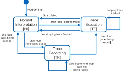
Execution is divided into three distinct execution phases: normal inter-pretation, in which the program is interpreted without the tracer interfering, trace recording, in which the operations of the interpreter are recorded by the tracing machine, andtrace execution, in which a previously recorded trace is executed. The execution phases and their transitions can be modeled as a state diagram, shown in Figure 2.
Normal Interpretation
[NI]
start-loop [no existing trace]
start-loop [existing trace] Guard failed Looping trace Þnished start-loop [label being traced] start-loop or end-loop [label not being traced] Trace Recording [TR] Trace Execution [TE] end-loop [label being traced]
Non-looping trace Þnished Program Start
Figure 2: The three execution phases of a program.
3.1. Tracer State
The tracer is modeled as a state machine transitioning between tracer states. Figure 1 lists the definitions of these states: a TracerState consists of a reference to the aforementioned execution phase, a tracer context, a program state, and a trace node.
During the execution of the program, the tracer switches between the ExecutionPhases: normal interpretation (NI), trace recording (TR) and trace execution (TE) phases. Section 3.3 describes the transitions between the different states of the tracer.
TheTracerContext is a two-tuple used by the tracer. The first component of the tuple stores the trace that is currently being recorded. This is either Null, if no trace is being recorded, or it is a trace node (TraceNode), which is a three-tuple that associates a trace with a unique label and a program state, so that this trace can later be retrieved by referencing its label. The second component, TraceNodeMap, stores all trace nodes, containing the traces that were previously recorded, by mapping the aforementioned labels to the trace nodes. The trace itself is a sequence of actions which are opaque interpreter-specific data structures that represent the operations performed by the interpreter while evaluating the program. When executing the trace, these same actions are again executed one-by-one by the interpreter. As these actions are unique to the interpreter that is used, they are not defined here. An example of some possible actions appeared in Listing 1b and is
shown again in Section 4, when discussing one possible implementation of the interpreter. However, we define one special end-trace actionetrp, whose
semantics are detailed in Section 3.3.
It is assumed that interpreters are modeled as state machines operating on a program state. This requirement enables the tracer to grab the entire, current execution state of the interpreter in the form of some program state which is defined by the interpreter and remains opaque to the tracer. The implementer of the interpreter could for example model the interpreter as a CESK machine. CESK-based interpreters operate on CESK states, consist-ing of a control component (C), an environment (E) (mappconsist-ing variables to addresses), a store (S) (mapping addresses to values) and a continuation stack (K) [12]. These interpreters are guided through the evaluation of a program by checking the state’s control component, which corresponds with either an expression to next be evaluated or a continuation to be followed. The state’s environment maps variables to addresses and its store maps these addresses to values. The continuation stack saves the continuations to be followed upon completing the evaluation of a (sub)expression and reaching a value. Abstracting a program’s execution as a program state facilitates transition-ing between the various phases of execution as both the execution of a trace and normal interpretation of the program operate on the same structure.
During the evaluation of the program, the interpreter operates on these program states and determines the next instruction, which, depending on the current execution phase, may be recorded into a trace by the tracing machine. The tracer obtains new program states from the interpreter during normal interpretation and trace recording, or by executing trace instructions during trace execution.
The last component of the tracer state either equals Null if no trace is currently being executed, or it contains the trace node storing the trace that is being executed.
3.2. Tracing Interface
Interpreter Functions. The tracing machine monitors and controls the ex-ecution of the interpreter through the following interface, which must be
provided by the interpreter:
step:ProgramState →InterpreterStep
applyAction:ProgramState ×Action →ActionReturn restart:RestartPoint ×ProgramState →ProgramState optimize:Trace×ProgramState →Trace
The tracer asks the interpreter to perform a single evaluation step on a program state via a two-step process. The tracer first calls thestepfunction on this state. In thisstepcall, the interpreter checks the state and considers which operations must be completed in this step of the evaluation. It then reifies these operations in the form of actions, i.e., data structures represent-ing the operations to execute, and wraps a list of the computed actions in an InterpreterStep. As the second step in the process, the tracer then makes the interpreter actually execute these reified operations by calling applyAction on them and the state to compute a ActionReturn that contains the new, updated program state. The restart function enables the tracer to restart normal interpretation when a guard failure has occurred at run time. The optimize function takes a trace and a program state and returns a trace that is optimized with respect to the given program state. It is designed such that the tracer can consider the optimization of a trace as a black box, rendering it the responsibility of the language implementer. In Section 4, we demonstrate how an interpreter that satisfies this interface may be built.
Note that although in principle the definitions of program states and actions are specific to one particular interpreter, in practice they might be reused between different interpreters, which in turn would enable language developers to also reuse at least the applyAction and optimize functions, similar to what is done in PyPy. However, creating a set of these common elements might place further constraints on the design of the interpreter, as the interpreter would have to accommodate for these components by adapting itsstepandrestartfunctions so that they employ these actions and states. Additionally, such a common program state should be sufficiently generic that it could be used by any sort of interpreter.
Program States. With the interpreter being a state machine, interpreting a program amounts to continuously executing the state transition rule that is applicable for the current program state; tracing the interpreter becomes recording the transitions performed by the interpreter state machine and
executing a trace corresponds to replaying the recorded transitions starting from the current program state. These transitions thus correspond to the aforementioned actions inSTRAF. Note that our tracer does not depend on
a particular definition for the program state or state transition, but this is left to the interpreter.
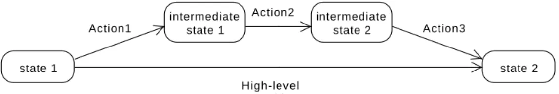
Actions. To enable a more fine-grained optimization of traces, the interpreter can use two sets of state transition rules: high-level and low-level transitions, i.e., actions, both operating on a program state. One high-level transition is composed of several low-level actions. As illustrated by Figure 3, executing the high-level transition is equivalent to applying each of the constituent actions consecutively. The high-level transition itself does not appear in a trace; only the low-level actions are recorded.
InterpreterStep. During the normal interpretation and trace recording phases, the tracing machine repeatedly asks the interpreter to perform a single high-level transition by calling step. This function takes the current program state as input and outputs an InterpreterStep: a two-tuple containing a list of actions to be applied on the given program state that together constitute the high-level transition that has just been performed, and possibly atracing signal. When the interpreter enters a loop, it communicates this to the tracer by including a tracing signal, startLoop, in its response. This enables the tracer to decide whether to start tracing this loop, start executing a previ-ously recorded trace for this loop, or do nothing at all. For this to work, the interpreter should identify each loop in the user program uniquely through a label. When interpreting a loop over multiple iterations, a startLoop is sent at the start of each iteration. If the tracer has started recording a loop after detecting astartLoopsignal at one iteration and subsequently detects anotherstartLoop for the same loop, it knows that one full iteration of the loop has been completed so it can stop recording. Conversely, when the in-terpreter exits a loop instead of continuing with another iteration, it includes the endLoop signal in the InterpreterStep. This enables the tracer to stop tracing in case it had been tracing this loop, so as not to traceoutside of the loop. We will call traces whose recording is stopped via such an endLoop signal non-looping traces in contrast to looping traces which are terminated via a startLoop. The difference between looping and non-looping traces is made more clear in Listing 2. Note that in Scheme, loops are constructed by recursively calling a function. Every function call could therefore loop back
(define (loop n) (loop (+ n 1)))
(a) A looping function; tracing will be
ter-minated via a startLoop.
(define (id x)
x)
(b) A non-looping function; tracing will
be terminated via anendLoop.
Listing 2: A looping versus a non-looping function.
High-level transition Action3 Action2 Action1 intermediate state 2 state 2 state 1 intermediate state 1
Figure 3: A high-level transition and corresponding actions.
to itself, so the interpreter sends anstartLoopat the start ofevery function call. Should the function indeed recursively call itself, as depicted in Listing 3a, a second startLoop will be sent and recording will be terminated. If no recursive call takes place, as is the case for Listing 3b, the interpreter sends a endLoop upon returning from the function call. Upon later execution of a non-looping trace, the tracer will restart normal interpretation when it reaches the end of the trace.
Note that in the basic model of STRAF, a nested loop will be inlined
when tracing the outer loop. However, it would be possible to extendSTRAF
such that this inlining is avoided, e.g., by aborting trace recording of an outer loop when an inner loop is detected.
Applying an Action. An action is applied by the tracer via the interface’s applyAction function. This returns an ActionReturn structure, which can be: an actionStep, a guardFailed or an endTrace. Most actions result in an actionStep, which wraps the new program state that is the result of applying the action on the input state. The purpose of guardFailed and endTracewill become clear over the next sections. Note that, in this model, guards are also a kind of action.
Guard Instructions. As a trace represents a single execution, guards are in-serted to ensure that a trace is only executed when the conditions that lead
to this specific path through the program are valid. Guards being actions themselves, when applied via applyAction, they cause the interpreter to check some condition on this state and then either return some actionStep in case the guard did not fail, or a guardFailed in case it did. The tracer detects this return value and takes action accordingly. As the generation and placement of guards is specific to the interpreted language, they need to be created by the interpreter during its processing of step requests and be included in the list of actions returned to the tracer via aninterpreterStep. Restarting Interpretation. Upon failure of a guard during the execution of a trace, or upon reaching the end of a non-looping trace, the tracer applies restart to the current program state and to a so-called restart point in order to restart normal interpretation. A restart point includes the necessary information to construct the program state from where normal interpretation must resume. Similar to actions and program states, the exact definition of a restart point intentionally depends on the interpreters. For the CESK example, a restart point could correspond to the control field of a state and point to the program expression that must now be evaluated; restart could then take this control and merge it with the other fields of the CESK state. Note that the design of correct restart points may depend on not only the interpreter that is used, but also on the optimizations employed by this interpreter, as the optimizations that are applied on a trace may have an effect on the restart points inside this trace. Similar to the process of optimizing traces, designing correct restart points, as well as ensuring that any interference between the trace optimizations and the restart points is resolved, is hence a responsibility of the interpreter developers.
3.3. Transition Rules
Figure 4 lists the formal semantics of the tracing machine and its in-teraction with the interpreter. We use this formalism to concisely describe the working of STRAF. A reference implementation for these semantics is
available at https://github.com/mvdcamme/scala-am.
These semantics center around how the TracerState of the tracing ma-chine is updated as execution of the program proceeds. For each rule, the first line matches the current configuration of the TracerState, the second line describes the updated TracerState. Subsequent lines describe conditions that must hold for for the original TracerState to transition such that it pro-duces this updated TracerState; specifically, the third line always indicates
what the result of the interpreter’s step function on the current program state must have been for this transition to take place. Note also that we use a helper functionapplyAction*which takes a program state and a sequence of actions as input and consecutively updates the program state with each action in the sequence, assuming the action resulted in an actionStep.
The helper function applyAction*can be recursively defined as follows: t is an empty list
applyAction*(s, t) = s applyActionEmpty applyAction(s, a) = actionStep(s′)
applyAction*(s, a :t) =applyAction*(s′, t) applyActionNonEmpty We also use the underscore character to match any field whose value is irrelevant. We use the notation T[lbl] to look up the label lbl in the map T. If the map does not contain this label, it returns an undefined value. Similarly, we use the notation T[lbl 7→tn] to either extend the map T with tn atlbl, ifT did not yet containlbl, or to replace the previous entry for lbl with the value tn.
Normal Interpretation. The normal interpretation phase (NI) refers to the execution stage in which no trace is being recorded or executed: the tracer only intervenes when the interpreter reaches the start of a loop, signaled by the interpreter via a TracingSignal, at which point the tracer may either decide to start tracing or to start executing a previously recorded trace. Figure 4a depicts the corresponding formalization.
Rule Ni-ContinueInterpreting represents the most common case in
which the interpreter either has not entered any loop, and the interpreter hence returns False instead of an actual signal, or the interpreter has exited a loop and it sends the endLoop tracing signal to indicate this. In both cases, the interpreter also returns the list of actions, t, that must be applied to arrive at the new program state, s′. As no actions are recorded while in the NI phase, the new tracer state is simply a copy of the old one, with the original program state replaced by the new one.
In rules NI-StartTracing and NI-StartExecuting, the interpreter
enters a loop that is identified by the label lbl. The first sequence of ac-tions, that are already part of the loop, consist of a1 : ... : an. In rule
NI-StartTracing, no trace has been recorded yet for this loop, so the tracer
step(s) = interpreterStep(t, signal)
signal equals either False orendLoop(lbl,rp)
ts(NI, tc, s, Null)→
ts(NI, tc, s′, Null)
NI-ContinueInterpreting
Where s’ = applyAction*(s, t)
step(s) = interpreterStep(a1 :...:an, startLoop(lbl)) T[lbl]is undefined ts(NI, tc(_, T), s, Null)→ ts(TR, tc(tn(lbl, a1 :...:an, s), T), s′, Null) NI-StartTracing Where s′ =applyAction*(s, a 1 :...:an)
step(s) = interpreterStep(_, startLoop(lbl))
T[lbl] =tn
ts(NI, tc, s, Null)→
ts(TE, tc, s, tn)
NI-StartExecuting
step(s) =interpreterStep(a1 :...:an, signal)
signal equals either False or startLoop(lbl′)or endLoop(lbl′,_) with lbl 6=lbl′ ts(TR, tc(tn(lbl, t, ss), T), s, Null)→
ts(TR, tc(tn(lbl, t :a1 :...:an, ss), T), s′, Null)
TR-ContinueTracing
Where s′ =applyAction*(s, a
1 :...:an)
step(s) = interpreterStep(t′, startLoop(lbl)) ts(TR, tc(tn(lbl, t, ss), T), s, Null)→ ts(TE, tc(Null, T[lbl 7→tn]), s′, tn) TR-SameStart Where s′ =applyAction*(s, t′) tn=tn(lbl, optimize(t,ss), ss) applyAction(_, etrp) =endTrace(rp) ApplyActionEndTrace
step(s) = interpreterStep(t′, endLoop(lbl,rp)) ts(TR, tc(tn(lbl, t, ss), T), s, Null)→ ts(NI, tc(Null, T[lbl 7→tn]), s′, Null) TR-SameEnd Where s′ =applyAction*(s, t′) tn=tn(lbl, optimize(t :etrp,ss), ss) (b) Trace recording
applyAction(s, a) =actionStep(s′) ts(TE, tc, s, tn(lbl, a :t, _))→ ts(TE, tc, s′, tn(lbl, t, _)) TE-NoSignal applyAction(s, a) =guardFailed(rp) ts(TE, tc, s, tn(lbl, a :t, _))→ ts(NI, tc, s′, Null) TE-GuardFailure Where s′ =restart(rp, s) applyAction(s, a) =endTrace(rp) ts(TE, tc, s, tn(lbl, a :t, _))→ ts(NI, tc, s′, Null) TE-TraceEnd Where s′ =restart(rp, s) T[lbl] =tn ts(TE, tc(tn, T), s, tn(lbl, φ, _))→ ts(TE, tc(tn, T), s, tn) TE-RestartLoop
Where φ represents the empty list
(c) Trace execution
starts tracing it: it changes its execution phase to indicate that it is now tracing, updates its tracer context by replacing the component representing its current trace and, as the sequence of actionsa1 :...:anis part of the loop
to be traced, it immediately records this sequence. The actions a1 : ...: an
are also applied to arrive at the new program state s′. This component now becomes a trace node consisting of the labellbl of the loop that is traced, the actions that were executed by the interpreter and that were carried back in the interpreterStep, as well as the old program states. sis saved so it can later be used as input for the optimizefunction, as described in Section 5.
In ruleNI-StartExecuting, the interpreter also starts a new loop
iter-ation, but the tracer context already contains a trace for this loop: i.e., it has an entry for the loop’s label lbl. The tracer switches its execution phase to TE to indicate it must execute this trace in the following step and the tracer replaces the trace node of the tracer state for the trace node containing the trace for the labellbl. As execution must now switch to the trace, the actions carried back in the interpreterStep are discarded entirely.
Trace Recording. In the trace recording phase (TR), all actions executed by the interpreter are recorded into a trace. Recording stops when the inter-preter sends either a startLoop signal or an endLoop signal carrying the same label as the trace being recorded. Figure 4b lists the corresponding rules.
Rule TR-ContinueTracing describes the situation where the
inter-preter has either not entered or exited a loop, or it has entered or exited a loop different from the one currently being traced, which is indicated by respectively the startLoop or endLoopcarrying a label different from the label of the loop being traced. In any case, the tracer records the interpreter’s actions by appending the list of actions a1 :... :an returned from the
inter-preter to the back of the trace. The program state is also replaced as the tracing process remains otherwise unaffected, the tracer continues tracing.
In rule TR-SameStart, the interpreter reaches the start of a loop, but
this loop has the same label as the one currently being traced. This means, one full iteration of the loop is completed and tracing can stop. The trace is then optimized, making use of the program state that was saved when start-ing the recordstart-ing of this trace, and stored in the tracer context. The actions t′ carried back in the interpreterStep are the same actions as those that were recorded at the beginning of the trace and are hence not recorded in the trace. Execution then continues by executing this optimized trace. Rule
TR-SameEnd describes the interpreter exiting a loop that is being traced,
instead of continuing with its next iteration. The interpreter sends an end-Loopsignal carrying the loop’s label and a restart pointrp. In response, the tracer appends the special end-trace action etrp to the end of the trace. The
semantics of this action are defined in the ApplyActionEndTrace rule:
when this action is executed via the applyAction function, applyAction always returns an endTrace structure carrying the communicated restart point. This restart point can then be used to restart normal interpretation from the point of the end of this loop.
Trace Execution. In the trace execution phase (TE), the tracer is executing a previously recorded trace. Figure 4c lists the corresponding rules. Note that a guard instruction is a normal action.
Rule TE-NoSignal describes the case where a non-guard action is
ap-plied, or a guard action that did not fail: an action from the trace is applied on the current program state, by callingapplyAction, and anactionStepis returned that contains the resulting program state. The tracer then continues by swapping its program state and moving on to the next action. In effect, this means that execution of each consecutive action in the trace happens via the interpreter.
Rule TE-GuardFailure describes a guard failure. Execution switches
back to normal interpretation, restarting from the point that corresponds with the guard failure. This point is determined by applyingrestarton the restart point given by the guard and the current program state, as described in Section 3.2.
In ruleTE-TraceEnd, the end of a non-looping trace has been reached.
The tracer restarts normal interpretation from some program point, deter-mined by calling the restartfunction on the current program state and the restart point associated with the end of the trace.
Rule TE-RestartLoop handles reaching the end of a regular, looping
trace, which means one full iteration of the loop is completed. The trace is restarted by looking up the full trace belonging to the label and replacing the current empty one.
3.4. Difference with Meta-tracing
Meta-tracing compilers, such as the RPython framework, do not directly trace the execution of a user-program, but rather trace the execution of a language interpreter,while this interpreter executes the user-program [4]. By
annotating their interpreters with certainhints [5], e.g., for detection of loops in the user-program, language developers can guide tracing and optimization of traces. The traces are then heavily optimized to produce efficient machine code corresponding to the relevant operations performed by the user pro-gram. This enables the interpreter’s implementers to employ the benefits of trace-based compilation without having to create their own dedicated trac-ing compiler. Furthermore, this makes it possible for developers to rapidly create interpreters with an acceptable performance level [16].
In STRAF, the tracing interface described in Section 3.2 enables
de-velopers to compose STRAF with any interpreter satisfying this interface.
The purpose of the tracing interface is also similar to the purpose of the hints provided in the language interpreters for the RPython framework. In these respects,STRAFresembles meta-tracing compilation frameworks such
as the RPython framework. However, although STRAF’s tracing interface
and RPython’s hints share the same purpose, their implementation and the extent to which both are used are significantly different.
The extent of the tracing interface is far greater than that of the RPython hints: the tracing interface not only enables detection of loops, but is also used to generate all instructions, including guard instructions, that must be recorded into the trace. This implies that, unlike meta-tracing, traces are interpreter-specific: instructions are not generated by the tracer but by the interpreter. As a consequence, the semantics of these instructions are gener-ally opaque to the tracer. Optimization of traces must therefore be performed by the interpreter, as opposed to the tracing compiler in the RPython frame-work, implying that a developer of an interpreter is also responsible for the optimization of traces.
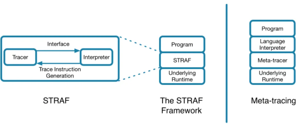
Figure 5 illustrates the difference between the STRAF framework and
a general meta-tracing compiler, such as the RPython framework. Whereas in meta-tracing, the language interpreter is generally described as running on top of the tracing compiler, in STRAF, the interpreter runs on the same
level as the tracer, with the tracer delegating regular program execution to the interpreter whenever required. Note also that the traces generated by
STRAF are not machine code, but that they are optimized sequences of
instructions to be executed by the interpreter.
Underlying Runtime Meta-tracer Language Interpreter Program Underlying Runtime STRAF Program Interface Tracer Interpreter Trace Instruction Generation The STRAF Framework Meta-tracing STRAF
Figure 5: The difference between the STRAFframework and a meta-tracing framework
4. Evaluating STRAF’s Generality
The strength of STRAFis its flexibility: it isgeneral with respect to the
set of interpreters that can be used, and it isextensible, i.e., the framework it-self can be extended with new features. Our evaluation of STRAFtherefore
focuses on evaluating these two aspects instead of, e.g., performance. Sec-tions 5 and 6 evaluateSTRAF’s extensibility. This section demonstrates the
generality of STRAF by constructing interpreters for two different
Scheme-like languages and integrating them intoSTRAF. This indicates that a
vari-ety of interpreters can be built that are in correspondence with the interface specified in Section 3.2 and, therefore, that STRAFdoes indeed accept
mul-tiple interpreters. At the same time, the presentation of these interpreters serves as a guide for how other suitable interpreters may be built.
4.1. Simple Scheme Interpreter
The first interpreter implements a non-trivial subset of the Scheme lan-guage. The interpreter is modeled after a variant of a CESK-machine [12] and hence satisfies the first requirement of our framework to model the in-terpreter as a state machine operating on some program state. Concretely, the program state consists of the standard control (C), environment (E), store (S), and continuation stack (K) components, as well as a value stack and value register. These last two components simplify implementing various transitions: the value register is used to store the value of the last evaluated subexpression, while the value stack is used to temporarily save the current environment as well as already evaluated arguments in a function call.
4.1.1. Evaluating Expressions
The interpreter determines how it should transition based on the content of its control component, which can either be an expression to be evaluated or a continuation to be followed. Thestepfunction of the interpreter checks the control and either calls stepEval with the expression to be evaluated or it calls stepKont with the corresponding continuation frame and the last value v that was evaluated. Both functions return an interpreterStep, as specified in the declaration of step in Section 3.2. Listing 3 exemplifies how an expression of the form (set! variable exp) is evaluated via the, partially elided, stepEvalfunction.
1 def stepEval(e: SchemeExp): InterpreterStep = e match {
2 ...
3 case SchemeSet(variable, exp) =>
4 val actions = ActionSaveEnv() ::
5 ActionEvalPush(exp, FrameSet(variable)) ::
6 Nil
7 InterpreterStep(actions, SignalFalse()) 8 }
9
10 def applyAction(state: ProgramState,
11 action: Action): ActionReturn = action match {
12 ...
13 case ActionEvalPush(exp, frame) =>
14 ActionStep(state.copy(control = ControlExp(exp),
15 kstack = state.kstack.push(frame)))
16 }
Listing 3: Evaluating aset!-expression.
In the case of aset! expression, the returnedinterpreterStep includes anActionSaveEnv(), for saving the current environment on the value stack, and an ActionEvalPush(exp, FrameSet(variable))), for simultaneously replacing the control component by the expression exp, as its value will have to be computed next, and pushing the continuation FrameSet on the continuation stack. Finally, the SignalFalse component indicates that the evaluation of a set! expression cannot trigger the beginning nor the end of a loop directly.
The returned actions are consecutively applied via theapplyAction func-tion. In the case of the Scheme interpreter, the actions are data structures to be interpreted. For example, an ActionEvalPush is handled by returning an actionStep (which is one possible ActionReturn) containing a copy of
the input program state with the continuation pushed onto the stack kstack and the control component replaced by the expression exp.
This example demonstrates how interpretation of a program can be de-composed into selecting which actions to use (step) and applying them (applyAction).
4.1.2. Loops
This subset of Scheme does not offer iterative looping constructs such as for. Loops in an execution therefore stem from recursion, as is the case for the factorial function depicted in Listing 4.
1 (define (fac n) 2 (if (< n 2)
3 1
4 (* n (fac (- n 1)))))
Listing 4: A factorial function.
Since the interpreter cannot generally know whether a function is recur-sive, it signals the possible start of a loop during the evaluation of every function application. Function application starts when all of its arguments are evaluated; arguments are evaluated by consecutively pushing and pop-ping FrameFunCallArgs continuation frames, as depicted in Listing 5. Each FrameFunCallArgs contains a reference to the evaluated operator, i.e., the function to be applied, and the list of arguments yet to be evaluated. If there is still an argument arg left to be evaluated, stepKont returns an ActionEvalPush to evaluate this argument next. If no arguments remain, the interpreter starts evaluating the function’s body: it moves to the first expression of the function’s body and it pushes a FrameFunBody to evaluate the rest of the body afterwards. Since this is the proper start of the func-tion applicafunc-tion, the interpreter passes a startLoop tracing signal along in the interpreterStep. The label of the signal corresponds to the AST of the body of the function to be applied. If this signal causes the tracer to start recording, tracing continues until the interpreter reaches the start of this function again, as this indicates that one iteration of the loop has been completed.
4.1.3. Non-Looping Traces
Listing 6 depicts how the endLoop tracing signal is sent when the in-terpreter reaches the end of a function application, i.e., when the list of
1 def stepKont(v: Value, frame: Frame): InterpreterStep = frame match {
2 ...
3 case FrameFunCallArg(fun, arg : args) => 4 val acts = ... :+
5 ActionEvalPush(arg, FrameFunCallArg(fun, args))) 6 InterpreterStep(acts, SignalFalse)
7 case FrameFunCallArg(fun, Nil) => 8 val acts = ... :+
9 ActionEvalPush(fun.body.head,
10 FrameFunBody(fun.body,
11 fun.body.tail)
12 InterpreterStep(acts, SignalStartLoop(functionValue.body)) 13 }
Listing 5: Evaluating a function application.
pressions still to be evaluated in the function’s body is Nil, while handling a FrameFunBodycontinuation frame. The label used in this signal is once more the full AST of the function’s body, which was passed via theFrameFunBody continuation. As specified in Section 3.3, an endLoop signal must carry a restart point for restarting normal interpretation after completing the execu-tion of the non-looping trace, so a RestartTraceEndedstructure is included in the signal.
1 def stepKont(v: Value, frame: Frame): InterpreterStep = frame match { 2 case FrameFunBody(body, Nil) =>
3 InterpreterStep(..., SignalEndLoop(body, RestartTraceEnded())) 4 }
Listing 6: Completing a function application.
4.1.4. Guards
Listing 7 shows how guard instructions are inserted into the trace in
STRAF. The listing depicts the evaluation of if-expressions, at the point
at which the predicate has already been evaluated.
The interpreter checks the value of the evaluated predicate and determines whether to evaluate the consequence or the alternative branch. It adds a guard instruction that corresponds to the taken branch: if the condition was true, the interpreter returnsActionGuardTrueand passes a reference to the other branch, i.e., the branch alt that was not taken.
Listing 8 shows how such an ActionGuardTrue is handled. When this guard instruction is reached during the execution of the trace, the value of
1 case class ActionGuardTrue(rp: RestartPoint) extends Action 2 case class RestartGuardIf(exp: SchemeExp) extends RestartPoint 3
4 def stepKont(v: Value, frame: Frame): InterpreterStep = frame match { 5 case FrameIf(cons, alt) =>
6 if (v.isTrue()) {
7 val actions = ActionGuardTrue(RestartGuardIf(alt)) :: ...
8 InterpreterStep(actions, SignalFalse) 9 } else { ... }
10 }
Listing 7: Continuing the evaluation of an if-expression.
the condition is stored in the value register, similar to how the condition’s value was stored there during the recording of the trace. The value register is therefore checked: if the value was againtrue, nothing needs to be done so an actionStep is returned. Otherwise, the guard has failed so a guardFailed is returned.
1 def applyAction(state: ProgramState,
2 action: Action): ActionReturn = action match {
3 case ActionGuardTrue(rp) => 4 if (state.v.isTrue()) { 5 ActionStep(this) 6 } else { 7 GuardFailed(rp) 8 } 9 }
Listing 8: Handling an ActionGuardTrue.
4.1.5. Restarting
Listing 9 depicts part of the interpreter’s implementation of the interface’s restartfunction, for generating new program states based on a restart point and the current program state. If the restart point is anRestartGuardIfFailed (cf. Listing 7), it contains a reference to the branch that wasnot taken dur-ing the recorddur-ing of the trace, and restart must only generate a copy of the input program state with its control component replaced by the given branch.
The implementation of guards and the restart function demonstrate that it is feasible to provide the functionality of trace guards by including a restart point structure and a restartfunction.
1 def restart(state: ProgramState,
2 rp: RestartPoint): ProgramState = rp match { 3 case RestartGuardIfFailed(exp) =>
4 state.copy(control = ControlExp(exp))
5 }
Listing 9: Partial implementation of the restartfunction.
4.2. Non-deterministic Ambeval Interpreter
To further demonstrate the generality of STRAF, we instantiate it with
a second interpreter: an implementation for Abelson and Sussman’s non-deterministic ambeval [1, Chapter 4].
4.2.1. Introduction
We first exemplify the non-determinism supported by this interpreter before discussing its implementation. Listing 10 shows a function that, upon exhaustive backtracking, returns all pairs of elements from two lists of which the sum is prime. It relies on the predefined function an-element-of which selects an element from the given list, and returns another element upon backtracking.
1 (define (prime-sum-pair list1 list2) 2 (let ((a (an-element-of list1)) 3 (b (an-element-of list2))) 4 (require (prime? (+ a b))) 5 (list a b)))
Listing 10: Example of a non-deterministic program [1, Chapter 4].
Ambiguous programs make use of a primitive amb expression, which se-lects a value among its arguments, creating a choice point in the execution of the program. The an-element-of function passes its input list to an amb expression to select some element from this list. require evaluates the given prime? predicate and causes evaluation of the program to fail when the predicate is false. When the program fails, execution backtracks to the last choice point: in this case, to the point where a value for the variable b was chosen. This causes b to be bound to a new element of the list. When no more elements remain, execution backtracks further to the definition of a where the process is repeated. The program can therefore be thought of as non-deterministic; any possible value is considered for each ambiguous
variable but only those values that satisfy all requirements are eventually used.
4.2.2. Implementation
The ambeval interpreter is challenging due to the possible interactions be-tween backtracking and tracing. Its implementation is modeled once more af-ter a CESK machine, with the exception that a separate failure continuation stack complements the regular continuation stack in the interpreter states. When the interpreter encounters an amb-expression, it pushes a FrameAmb continuation on this new stack. When execution fails, the interpreter pops a continuation from this same stack such that it can continue from the last amb-expression with another value.
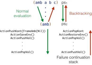
To restart execution from the last amb-expression, the interpreter must undo any changes made in the meantime. For instance, variables that have since been defined should be removed from the environment. To enable undo-ing such actions, for each action that is applied, an opposite action is wrapped in a FrameUndoAction and pushed onto the failure continuation stack, as il-lustrated by Figure 6. When a failure is triggered, the interpreter executes the undo-actions saved on the failure stack, thereby restoring the program state from the time at which the amb-expression it is restarting from was evaluated. Eventually, the interpreter will pop the FrameAmb continuation from the stack, at which point stack rewinding is complete.
In general, adapting the interpreter such that it saves these undo-actions on the failure continuation stack does not interfere with tracing. The am-beval interpreter traces functions in a way that is identical to the previous interpreter: by sending a startLoop signal to the tracer upon entering the body of a function and sending an endLoop signal upon its exit. However, care must be taken during stack rewinding when a function is being traced. If the execution were to backtrack behind the function call that is being traced, tracing should be aborted as this situation is similar to exiting from a func-tion before the funcfunc-tion loops. Listing 11 exemplifies how undo-acfunc-tions are applied and how the endLoopsignal is sent.
Section 4.1.2 explained that the interpreter pushes aFrameFunBodyonto the regular continuation stack when starting a function application. When this continuation is therefore popped again while backtracking, the inter-preter has reached the point in the program at which it started evaluating the function application. If the tracer is tracing the function application that it is now returning from, tracing should stop here, as it would backtrack
(amb a b c) . . . (amb) ActionPushKont(FrameAmb(Nil)) ActionSaveEnv() ActionPushVal() . . . ActionPopVal() ActionPopKont ActionRestoreEnv() ActionPopVal() . . . ActionPushVal() Failure continuation stack ps1 ps2 Normal evaluation Backtracking
Figure 6: Undoing actions after execution has failed.
1 def stepKont(v: Value, frame: Frame): InterpreterStep = frame match { 2 // Rewinding the failure continuation stack
3 case FrameUndoAction(reverseAction) => reverseAction match { 4 // Undoing a push-continuation
5 case ActionPopKont() => getTopKont() match {
6 // Undoing a push of a FrameFunBody continuation 7 case FrameFunBody(body, Nil) =>
8 InterpreterStep(..., SignalEndLoop(body, RestartTraceEnded()))
9 }
10 }
11 }
Listing 11: Backtracking out of an function application.
out of the function otherwise. The interpreter therefore sends an endLoop signal with a restart point of the form RestartTraceEnded.
No further changes need to be made to this Ambeval interpreter to make it satisfy the required interface.
4.3. Conclusion
The interpreters presented here demonstrate the variety of interpreters that can be plugged intoSTRAF, and exemplify executable implementations
of the structures and signals described in Section 3.2. Together, they serve to demonstrate the generality of STRAF: its tracer can be reused to construct
runtimes for different languages.
5. Optimizing Traces
We now provide a first demonstration of STRAF’sextensibility by using
its optimize hook to implement a set of optimizations that are common in the literature. For brevity, we give only a high-level description of the added optimizations, but their implementation is available online.2
The traces on which we apply these optimizations are recorded by the simple Scheme run-time presented in Section 4.1.
Optimization of traces is encoded in the interpreter’s interface via the optimizefunction, which takes a trace as input as well as the program state that was observed by the tracing machine when it started recording the given trace. As the application of actions is deterministic,3
saving the program state that was observed at the start of the trace recording enables the opti-mizer to reconstruct, if necessary, each program state as it could have been observed while applying the corresponding actions during the recording of the trace. These program states provide the optimizations with all available concrete information, such as the contents of the store and the environment and hence the values that were observed for all variables in the program. The states can be discarded after completing the optimizations.
We implemented six different optimizations. Four of these represent well-known and widely used optimizations in the domain of (trace-based) JIT compilation:
Constant folding (O1) [9] Applications of arithmetic primitives that only use constants as arguments are replaced by the resulting value.
Arithmetic operations type specialization (O2) [7] Applications of generic arithmetic primitives, e.g., a generic plus operation, are optimistically replaced by the equivalent type-specialized operation, e.g., a plus oper-ation specialized for floating point operands, if it was observed that all of its arguments belong to the same type. A guard is inserted to verify whether the types of the arguments remain the same at run time. Variable folding (O3) The set of all free variables in a trace, i.e., the set
of variables that are neither defined nor assigned to inside the trace,
2
https://github.com/mvdcamme/scala-am/blob/master/src/main/scala/ tracing/SchemeTraceOptimizer.scala
3
In practice, there are some instances of non-determinism, e.g.,random, so the frame-work includes additional information for some actions while recording a trace.
is computed. The trace is extended with a loop-invariant header con-taining, for each variable, an action for saving the current value of the variable in a specified register. Eachread instance of these variables is then replaced by an action for looking up this variable in the register, thereby avoiding a more costly double lookup of the variable through the environment and the store.
Action merging (O4) Some actions that are likely to appear immediately behind each other in a trace are merged. Applying the merged action then has the same result as applying both actions separately. Increasing the granularity of actions decreases the total time spent in dispatching actions. For example, an action for looking up a value could in practice likely be followed by an action for popping a continuation from the continuation stack; these actions could hence be merged into one action to perform both operations. The effect of the granularity of opcodes in traces was previously described in [8].
In addition, we implemented two optimizations that respectively remove redundant saves and restores of the environment (O5), and pushes and pops of the continuation stack (O6).
Listing 12 demonstrates how the type specialization optimization, can be implemented and how it uses the starting program state to compute the state that would have been recorded foreach action in the trace. This state is then used to retrieve the operands of arithmetic operations. The optimization then checks whether each operand is of the same type and if so replaces the generic operation by its equivalent type-specialized operation instead.
The actual optimize function pipelines each of these six optimizations, passing along its input program start state to each individual optimization that requires it. The purpose of adding these optimizations is not to provide a performant execution environment for Scheme, but to demonstrate that
STRAFis sufficiently extensible to support them. The optimizehook with
its two input parameters sufficed to implement all six optimizations, without requiring changes to the framework itself. All implementations together, moreover, amount to a mere 500 lines of Scala code.
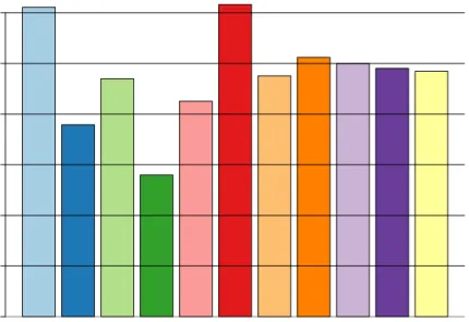
5.1. Benchmark Results
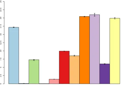
To illustrate the effectiveness of the listed optimizations, we include Fig-ure 7, depicting the median time required, with the 95% confidence intervals
1 def typeSpecialize(trace: Trace, start: ProgramState): Trace = {
2 /*
3 * replaceActions takes as input a tuple of an action in the
4 * trace and its associated program state (i.e., the state achieved 5 * by consecutively applying each action up til now in the trace 6 * on the given start-state) and returns either a new, more specific, 7 * action if the action corresponds to the application of an
8 * arithmetic operation on a set of operands all of the same type, 9 * or the same action otherwise.
10 */
11 def replaceAction(tuple: (Action, ProgramState)): Action = {
12 val (action, state) = tuple
13 // The operands are saved on the stack in the state
14 val operands = getOperands(action, state)
15 if (isArithmeticOperation(action) && (allSameType(operands)) { 16 // We call replaceOperation to replace this action
17 // with its equivalent, type-specialized action. 18 // The generation of a guard is not depicted here.
19 replaceOperation(action, typeOf(operands))
20 // Action cannot be specialized
21 } else {
22 action
23 }
24 }
25 // We compute the consecutive program states that correspond 26 // with applying each action in the trace via weaveStates, zipping 27 // program states and actions together.
28 val zipTrace: List[(Action, ProgramState)] = weaveStates(trace, start) 29 zipTrace.map(replaceAction) }
Listing 12: Pseudo-implementation of type specialization.
included, forSTRAFto execute a set of benchmarks when no optimizations
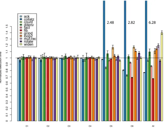
are applied. These results serve as the baseline for Figure 8, which depicts the median execution time, normalized with respect to this baseline, of exe-cuting the same benchmarks, first with each of the six optimizations enabled individually (O1-6), and finally with all optimizations enabled (All).
The benchmarks were executed on an Intel I7-4870HQ CPU at 2.50GHz with 6MB cache and 16GB RAM, running 64bit OS X 10.11.4 and Scala 2.11.7 on the Java Hotspot VM 25.92. Each benchmark is executed 30 times in a separate JVM. Measurements are taken after JVM warmup was completed: we observed stable measurements after two iterations of execution of the pro-gram. The median of the results and its 95%-confidence interval are reported.
While executing these benchmarks, we used the tracing compilation features described in Section 6 by defining a tracing threshold of 10 and enabling guard tracing.
The results show that the first four optimizations generally do not pro-vide significant performance improvements. Removing redundant saves and restores of the environment (O5) and removing redundant pushes and pops of continuation frames (O6), do offer a small performance increase in some cases. Notably, the collatz benchmark is significantly slower when applying these two optimizations. This benchmark produces one large trace of which the execution always leads to a guard failure quickly. Thus, the overhead of applying both optimizations on this trace is never recouped, as execution of the trace is quickly aborted.
ack collatz count dderiv fact fib gcipd loop2 mut−rec rotate widen Baseline Execution Time
Benchmark
Median Ex
ecution Time (seconds)
0 2.5 5 7.5 10 12.5 15 17.5 20 22.5 25
Figure 7: Median execution time for the baseline execution (no optimizations applied).
O1 O2 O3 O4 O5 O6 All N o rma li z e d e x e cu ti o n t ime 0 0 .1 0 .2 0 .3 0 .4 0 .5 0 .6 0 .7 0 .8 0 .9 1 1 .1 1 .2 1 .3 1 .4 1 .5 2.48 2.82 6.28
Figure 8: Normalized execution times with each of the six optimizations applied individ-ually (O1-6), and with all optimizations applied (All).
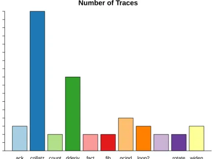
Figure 9 depicts the total number of traces that were recorded during the execution of each benchmark. This number includes both regular traces and traces produced after a guard failure has occurred (see Section 6.2). Note that both the trace recording and optimization process as well as the bench-marks themselves are completely deterministic. The number of recorded traces therefore does not vary over time. Also note the high number of (guard) traces produced by the collatz benchmark indicating that traces are quickly aborted due to failing guards, which in turn leads to more traces being recorded, so that the computational overhead of optimizing the trace is never recouped.
Regardless of their effectiveness, adding these optimizations to STRAF
indicates that the framework is extensible, and that optimizations can be implemented by using the optimizehook.
ack collatz count dderiv fact fib gcipd loop2 rotate widen Number of Traces Benchmark Number of T races 0 1 2 3 4 5 6 7 8 9 10 11 12 13 14 15 16 17
Figure 9: The total number of traces recorded during the execution of the benchmark.
5.2. Additional Performance Metrics
Since we experiment with a highly conceptualized and thus comparably inefficient interpreter, the optimizations are not as effective as they are in optimized systems. Inspired by Brunthaler [6], we thus also measure their effects on a different set of metrics beside performance and we compare with the baseline, unoptimized execution of the benchmarks. This gives us a notion of the effect of the optimizations on the traces.
1. The effectiveness of the action merging optimization (O4), the removal of redundant environment saves and restores (O5), as well as the re-moval of redundant continuation pushes and pops (O6), is measured by total length of the generated traces. For brevity, we only report the combination of the three optimizations.
2. The type specialization (O2) optimizations is measured by the number of non-type specialized arithmetic operations that are applied.
3. The variable folding optimization (O3) is measured by the number of variable lookups.
Note that all figures depicting the baseline results use a log-scaled y-axis. 33
5.2.1. Trace lengths
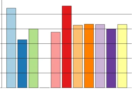
Figure 10b illustrates that the action merging optimization, the removal of redundant environment saves and restores and the removal of redundant continuation pushes and pops is effective at reducing the length of traces by at least 50% in all cases.
5.2.2. Generic arithmetic operations
Figure 11 depicts the total number of generic, non-type-specialized arith-metic operations that are executed during the total lifetime of each pro-gram, both while executing a trace or while interpreting the program. When enabling the type-specialization optimization (Figure 11b) the number of generic operations that are executed in the ack, count, loop2, mut-rec and rotate programs, drops down to almost zero, as all arithmetic operations that take place in a trace are successfully type-specialized. The only generic arithmetic operations left for these benchmarks are those that are executed outside of a trace. In the case of the fact, fib, gcipd and widen benchmarks, the number of generic arithmetic operations also significantly decreases. As the dderiv benchmark does not use any arithmetic operations inside a traced part of the program, the optimization is ineffective.
5.2.3. Variable Lookups
Figure 12 depicts the total number of times a variable is looked up during the execution of each program, again both while executing a trace and while interpreting the program. As the variable folding optimization avoids lookups of free variables in the trace by placing these variables in read-only registers before executing the trace, we expect the number of variable lookups to drop significantly, depending on the amount of free variables. As shown in Figure 12b, the number of variable lookups indeed significantly drops across all benchmarks, from 13% for the collatz benchmark, to 67% for the fact benchmark.
5.2.4. Constant Folding
In the case of this limited set of benchmarks, the constant folding opti-mization has no effect on any benchmark, as none of the programs contain any arithmetic expression that only makes use of constant values.
35
ack collatz count dderiv fact fib gcipd loop2 rotate widen
Baseline Trace Lengths
Benchmark
T
otal T
race Lengths (Number of Instr
uctions) 1e+00 1e+01 1e+02 1e+03 1e+04
(a) The total, combined length of all recorded traces when no optimizations have been enabled.
ack collatz count dderiv fact fib gcipd loop2 rotate widen
Normalized Trace Lengths
Benchmark Nor maliz ed T race Lengths 0 0.1 0.2 0.3 0.4 0.5 0.6 0.7 0.8 0.9 1
(b) The total, combined length of all recorded traces (normalized to Figure 10a)
with optimizations O4,O5 andO6 have all been enabled.
36
ack collatz count dderiv fact fib gcipd loop2 rotate widen
Generic Primitive Calls
Benchmark Number of Gener ic Pr imitiv e Calls 1e+00 1e+01 1e+02 1e+03 1e+04 1e+05 1e+06
(a) The number of generic, i.e., not type-specialized, arithmetic operations when no optimizations are enabled.
ack collatz count dderiv fact fib gcipd loop2 rotate widen
Normalized Generic Primitive Calls
Benchmark Nor maliz ed Number of Gener ic Pr imitiv e Calls 0 0.1 0.2 0.3 0.4 0.5 0.6 0.7 0.8 0.9 1
(b) The number of generic, i.e., not type-specialized, arithmetic operations
(nor-malized to Figure 11a) with only optimization O2 enabled.
37
ack collatz count dderiv fact fib gcipd loop2 rotate widen
Variable Lookups Benchmark Number of V ar iab le lookups 1e+00 1e+01 1e+02 1e+03 1e+04 1e+05 1e+06
(a) The number of variable lookups when no optimizations are enabled.
ack collatz count dderiv fact fib gcipd loop2 rotate widen
Normalized Variable Lookups
Benchmark Nor maliz ed Number of V ar iab le Lookups 0 0.1 0.2 0.3 0.4 0.5 0.6 0.7 0.8 0.9 1
(b) The number of variable lookups (normalized to Figure 12a) with only
optimiza-tion O3 is enabled.
6. Evaluating STRAF’s Adaptability
This section evaluatesSTRAF’sextensibility by adding two mechanisms
that are widely used in trace-based JIT compilers. Specifically, we add a heuristic for detecting hot loops and a mechanism for starting traces from guard failures. These mechanisms build on the framework itself, so we de-scribe them as variations on the semantics presented in Section 3, although they are directly included in our implementation. By demonstrating how
STRAFcan be extended with these features, we provide an intuition of the
effort for further extending or adapting STRAF. As we will show, including
these mechanisms requires only minimal changes. 6.1. Hot Loop Detection
Tracing compilation is most effective when applied to the parts where a program spends most of its time (i.e., the hot parts) [14]; optimizing rarely executed parts can reduce overall performance, because of the time it takes to do the tracing and optimizations [13].
InSTRAF, tracing of a loop starts immediately once this loop is executed
for the first time. Although this is adequate for a basic implementation, it does not correspond well to the state-of-the-practice in tracing JIT compilers. Therefore, the first evaluation of the adaptability of STRAF is a heuristic
to detect hot loops in a program’s execution. A program loop is called “hot” once it has been completed at least a fixed amount of times, i.e., once a threshold has been exceeded. This type of hot loop detection is used for instance in HotpathVM [13], TraceMonkey [14], and SPUR [3].
6.1.1. Extending the Tracing Machine
To detect hot loops, we extend the tracing machine to count the number of iterations that have been completed for each loop, as shown in Figure 13. To this end, our extension implements a LabelCounterMap that associates a trace label to a counter, similar to how TraceNodeMap associates a label to a trace node. When the interpreter enters a loop, i.e., when it sends the startLoop signal, the counter for the loop’s label is updated.
6.1.2. Semantics
To add hot loop detection, we need to adapt the tracing semantics. Specif-ically, we need to change how tracing is started, i.e., how we transition from the normal interpretation phase of trace execution to the trace recording