A Bayesian hierarchical model for comparing average F1 scores

A Bayesian Hierarchical Model for Comparing Average F1 Scores

Dell Zhang DCSIS

Birkbeck, University of London Malet Street

London WC1E 7HX, UK Email: [email protected]

Jun Wang, Xiaoxue Zhao Dept of Computing Science University College London

Gower Street London WC1E 6BT, UK Email:{j.wang,x.zhao}@cs.ucl.ac.uk

Xiaoling Wang Software Engineering Institute East China Normal University 3663 North Zhongshan Road

Shanghai 200062, China Email: [email protected]

Abstract—In multi-class text classification, the performance (effectiveness) of a classifier is usually measured by micro-averaged and macro-micro-averaged F1 scores. However, the scores themselves do not tell us how reliable they are in terms of forecasting the classifier’s future performance on unseen data. In this paper, we propose a novel approach to explic-itly modelling the uncertainty of average F1 scores through Bayesian reasoning, and demonstrate that it can provide much more comprehensive performance comparison between text classifiers than the traditional frequentist null hypothesis significance testing (NHST).

Keywords-text classification; performance evaluation; hy-pothesis testing; model comparison; Bayesian inference

I. INTRODUCTION

Automatic text classification [1] is a fundamental tech-nique in information retrieval (IR) [2]. It has many important applications, including topic categorisation, spam filtering, sentiment analysis, message routing, language identification, genre detection, authorship attribution, and so on. In fact, most modern IR systems for search, recommendation, or advertising contain multiple components that use some form of text classification.

The most widely used performance measure for text clas-sification is theF1score [3] which is defined as the harmonic mean of precision and recall. It is known to be more informative and more useful than classification accuracy etc. due to the prevalent phenomenon of class imbalance in text classification. When multiple classes exist in the document collection (such as Reuters-21578 with its 118 classes), we often want to compute a single aggregate measure that combines theF1scores for individual classes. There are two methods to do this: micro-averaging and macro-averaging [2]. The former pools per-document decisions across classes, and then computes the overall F1 score on the pooled contingency table. The latter just computes a simple average of theF1scores over classes. The differences between these two averaging methods can be large: micro-averaging gives equal weight to each per-document classification decision and therefore is dominated by large classes, whereas macro-averaging gives equal weight to each class. It is nowadays a common practice for IR researchers to evaluate a

multi-class text multi-classifier using both the micro-averagedF1score (denoted as miF1) and the macro-averaged F1 score (de-noted as maF1), since their introduction by Yang and Liu’s seminal SIGIR-1999 paper [4].

However, the averageF1 scores themselves only reflect a text classifier’s performance on the given test data. How can we be sure that it will work well on unseen data? Given any finite amount of test results, we can never be guaranteed that one classifier’s performance will definitely achieve a certain acceptable level (say 0.80) in practice. For example, suppose that a classifier got miF1 0.81 on 100 test documents. Due to the small number of test documents, we probably do not have much confidence in pronouncing that its future performance will definitely be above 0.80. If instead the classifier got miF10.81 on 100,000 test documents, we can be more confident than in the previous case. Nevertheless, there will always be some degree of uncertainty. The central question here is how to assess the uncertainty of a classifier’s performance as measured by miF1 and maF1. Perhaps the simplest solution is to applyk-fold cross-validation [5] and then calculate the sample variance of average F1 scores over multiple “folds” of the dataset. This method tends to yield poor estimations though: the sample variance can approximate the true variance well only if we have a large number of folds, but when the dataset is divided into many folds, the size of each fold is likely to be too small to give a meaningful averageF1score. Hence it is desirable to derive the uncertainty of average F1 scores directly from all the atomic document-category classification results.

In this paper, we build up on our previous preliminary work [6] to address this problem through Bayesian hierar-chical modelling [7], [8], and demonstrate that our proposed Bayesian approach can provide much more comprehensive performance comparison between text classifiers than the traditional frequentist null hypothesis significance testing (NHST).

The rest of this paper is organised as follows. In Sec-tion II, we review the existing approaches to the problem of classifier performance comparison. In Section III, we present our Bayesian estimation based approach in detail. In Section IV, we show how the proposed approach can be used

to compare some well-known text classification algorithms. In Section V, we discuss several natural extensions to the proposed approach. In Section VI, we draw conclusions.

II. RELATEDWORK A. Frequentist Performance Comparison

The traditional frequentist approach to comparing clas-sifiers is to use NHST [5]. The usual process of NHST consists of four steps: (1) formulate the null hypothesisH0 that the observations are the result of pure chance and the alternative hypothesisH1 that the observations show a real effect combined with a component of chance variation; (2) identify a test statistic that can be used to assess the truth of H0; (3) compute thep-value, which is the probability that a test statistic equal to or more extreme than the one observed would be obtained under the assumption of hypothesisH0; (4) if thep-value is less than an acceptable significance level, the observed effect is statistically significant, i.e.,H0is ruled out andH1is valid.

Specifically for performance comparison of text classi-fiers, the usage of NHST has been presented in detail by Yang and Liu in their SIGIR-1999 paper [4]. In summary, on the document level (micro level), sign-test can be used to compare two classifiers’ accuracy scores (called s-test), while unpairedt-test can be used to compare two classifiers’ performance measures in the form of proportions, e.g., precision, recall, error, and accuracy (called p-test); on the category level (macro level), sign-test and paired-t test can both be used to compare two classifiers’ F1 scores (which are called S-test and T-test respectively).

In spite of being useful and influential, such a frequentist approach unfortunately has many inherent deficiencies and limitations [8], [9]. To name a few: (i) NHST is only able to tell us whether the experimental data are sufficient to reject the null hypothesis (that the performance difference is zero) or not, but there is no way to accept the null hypothesis, i.e., it is impossible for us to confidently claim that two classifiers perform equally well; (ii) NHST will reject the null hypothesis as long as the experimental data suggest that the performance difference is non-zero, even if the performance difference is too slight to have any real effect in practice; (iii) complex performance measures such as theF1score can only be compared on the category level but not on the document level, which seriously restricts the statistical power of NHST as the number of categories is usually much much smaller than the number of documents. The other NHST methods that have been applied to compare classifiers include ANOVA test [10], Friedman test [11], McNemar’s test [12], and Wilcoxon signed-rank test [13]. Due to their frequentist nature, no matter which specific test they use, more or less they suffer from the above mentioned perils.

B. Bayesian Performance Comparison

1) Bayes Factor: Model comparison using Bayes factor has been applied to the problem of classifier performance comparison [14], [15]. In our context, the Bayes factor is the marginal likelihood of classification results data for the null model Pr[D|M0] (where two classifiers perform equally well) relative to the marginal likelihood of clas-sification results data for the alternative model Pr[D|M1] (where one classifier works better than the other classifier): BF= Pr[D|M0]/Pr[D|M1].

As the BF becomes larger, the evidence increases in favour of modelM0 over model M1. The rule of thumb for interpreting the magnitude of the BF is that there is “substantial” evidence for the null model M0 when the BF exceeds3, and similarly, “substantial” evidence for the alternative modelM1 when the BF is less than 1₃.

Although for simple models the value of Bayes factor can be derived analytically as shown by [14]–[17], for complex models it can only be computed numerically using for example the Savage-Dickey (SD) method [18]–[20]. The SD method assumes that the prior on the variance in the null model equals the prior on the variance in the alternative model at the null value:Pr[σ2_|M

0] = Pr[σ2|M1, δ = 0]. From this it follows that the likelihood of the data in the null model equals the likelihood of the data in the alternative model at the null value: Pr[D|M0] = Pr[D|M1, δ = 0]. Thus, the Bayes factor can be determined by consider-ing the posterior and prior of the alternative hypothesis alone, because the Bayes factor is just the ratio of the probability density at δ = 0 in the posterior relative to the probability density at δ = 0 in the prior: BF = Pr[δ = 0|M1,D]/Pr[δ = 0|M1]. The posterior density Pr[δ= 0|M1,D] and the prior density Pr[δ= 0|M1] can both be approximated by fitting a smooth function to the Markov Chain Monte Carlo (MCMC) [7], [8] samples via kernel density estimation (KDE) etc.

This approach largely avoids the above mentioned perils of NHST, except for the third one on complex performance measures. However, it is known that the value of Bayes factor can be very sensitive to the choice of prior distribution in the alternative model [9]. Another problem with Bayes factor is that the null hypothesis can be strongly preferred even with very few data and very large uncertainty in the estimate of the performance difference [9]. Furthermore, generally speaking, a single Bayes factor is much less informative than the entire posterior probability distribution of the performance difference provided by our Bayesian estimation based approach.

2) Bayesian Estimation: It has been loudly advocated in recent years that the Bayesian estimation approach to comparing two groups of data has many advantages over using NHST or Bayes factor [8], [9]. However, to our knowledge, almost all the existing models of Bayesian

ˆ y 1 · · · k · · · M y 1 .. . . .. j cjk cj θj .. . . .. M

Figure 1: A schematic diagram of confusion matrix.

estimation deal with continuous values (that can be described by Gaussian ortdistributions) but not discrete classification outcomes, and they produce estimations for simple statistics (such as the average difference between the two given groups) but not complex performance measures (such as the F1 score). Probably the most closely related work is that of Goutte and Gaussier [21] (which has been brought to our attention by the reviewers). Their F1 score model constructed using a couple of Gamma variates is not as expressive and flexible as ours. It is restricted to a single F1 score for binary classification with two classes only. In contrast, our proposed approach opens up many possibilities for adaptation or extension.

III. OURAPPROACH A. Probabilistic Models

Let us consider a multi-class classifier which has been tested on a collection of N labelled test documents, D. Here we focus on the setting of multi-class single-label (aka “one-of”) classification where one document belongs to one and only one class [1], [2]. For each document xi

(i = 1, . . . , N), we have its true class label yi as well as

its predicted class labelyˆi. Given that there areM different

classes, the classification results could be fully summarised into anM×M confusion matrixC where the elementcjk

at thej-th row and thek-th column represents the number of documents with true class labeljbut predicted class label k, as shown in Fig. 1.

The performance measures miF1 and maF1 can be cal-culated straightforwardly based on such a confusion matrix. However, as we have explained earlier, we are not satisfied with knowing only a single score value of the performance measure, but instead would like to treat the performance measure (either miF1 or maF1) as a random variable ψ and estimate its uncertainty by examining its posterior probability distribution.

The test documents can usually be considered as “inde-pendent trials”, i.e., their true class labelsyiare independent

and identically distributed (i.i.d.). For each test document, we use µ = (µ1, . . . , µM) to represent the probabilities

that it truly belongs to each class: µj = Pr[yi = j]

(j = 1, . . . , M), PM_j=1µj = 1. This means that the

class sizesn= (n1, . . . , nM) would follow a Multinomial

distribution with parameterN andµ:n∼Mult(N,µ), i.e.,

Pr[n|N,µ] = N! n1!. . . nM! M Y j=1 µnj j = ΓPM_j=1(nj+ 1) QM j=1Γ(nj+ 1) M Y j=1 µnj j . (1)

It would then be convenient to use the Dirichlet distribution (which is conjugate to the Multinomial distribution) as the prior distribution of parameter µ. More specifically, µ ∼ Dir(β), i.e., Pr[µ] = ΓPM_j=1βj QM j=1Γ(βj) M Y j=1 µβj−1 j , (2)

where the hyper-parameter β = (β1, . . . , βM) encodes

our prior belief about each class’s proportion in the test document collection. If we do not have any prior knowledge, we can simply set β = (1, . . . ,1) that yields a uniform distribution, as we did in our experiments.

Furthermore, letcj = (cj1, . . . , cjM)denote thej-th row

of the confusion matrix. In other words,cjshows how those

documents belonging to classj are classified. For each test document from that classj, we useθj = (θj1, . . . , θjM)to

represent the probabilities that it is classified into different classes: θjk = Pr[ˆyi = k|yi = j] (k = 1, . . . , M), PM

k=1θjk= 1. This means that for each classj, the

corre-sponding vectorcj would follow a Multinomial distribution

with parameternj andθj:cj∼Mult(nj,θj), i.e.,

Pr[cj|nj,θj] = nj! cj1!. . . cjM! M Y k=1 θcjk jk = ΓPM_k=1(cjk+ 1) QM k=1Γ(cjk+ 1) M Y k=1 θcjk jk . (3)

It would then be convenient to use the Dirichlet distribution (which is conjugate to the Multinomial distribution) as the prior distribution of parameter θj. More specifically,θj ∼

Dir(ωj), i.e., Pr[θj] = ΓPM_k=1ωjk QM k=1Γ(ωjk) M Y k=1 θωjk−1 jk , (4)

where the hyper-parameter ωj = (ωj1, . . . , ωjM) encodes

our prior belief about a classifier’s prediction accuracy for class j.

Moreover, we introduce a higher-level overarching hyper-parameter η to capture the overall tendency of making correct predictions. In other words, we assume that ωjj,

the prior probability of correctly assigning a document of class j to its true class j, would be governed by the same

hyper-parameter η for all the classes. Thus for class j, we setωjk=η ifj =k andωjk= (1−η)/(M−1)if j6=k.

The hyper-parameterηitself can be considered as a random variable that ranges between 0 and 1, so it is assumed to follow a Beta distribution. More specifically,η ∼Beta(α), i.e.,

Pr[η] = Γ(α1, α2) Γ(α1)Γ(α2)

µα1−1_(1−µ)α2−1 _{, (5)}

where the hyper-parameterα= (α1, α2)encodes our prior belief about the average classification accuracy of the given classifier. If we do not have such knowledge, we can simply setα= (1,1) that yields a uniform distribution, as we did in our experiments. Such a Bayesianhierarchicalmodel [7], [8] is more powerful as it allows us to “share statistical strength” across different classes.

Once the parameters µ and θj (j = 1, . . . , M) have

been estimated, it will be easy to calculate, for each class, the contingency table of “expected” prediction results: true positive (tp), false positive (f p), true negative (tn), and false negative (f n). For example, the anticipated number of true positive predictions, for class j, should be the number of test documents belonging to that class N µj times the rate

of being predicted by the classifier into that class as well θjj. The equations to calculate the contingency table for

each classj are listed as follows.

tpj=N µjθjj f pj= X u6=j N µuθuj f nj= X v6=j N µjθjv tnj= X u6=j X v6=j N µuθuv

Inmicro-averaging, we pool the per-document predictions across classes, and then use the pooled contingency table to compute the micro-averaged precisionP, micro-averaged recallR, and finally their harmonic mean miF1 as follows.

P = PM j=1tpj PM j=1(tpj+f pj) = M X j=1 µjθjj (6) R = PM j=1tpj PM j=1(tpj+f nj) = M X j=1 µjθjj (7) miF1= 2P R P+R = M X j=1 µjθjj (8)

It is a well-known fact that in multi-class single-label (aka “one-of”) classification, miF1 =P =R which is actually identical to the overall accuracy of classification [2].

Inmacro-averaging, we use the contingency table of each individual classjto compute that particular class’s precision Pjas well as recallRj, and finally compute a simple average

M ψ cj θj N µ ωj β η α n

Figure 2: The probabilistic graphical model for estimating the uncertainty of averageF1 scores.

of theF1 scores over classes to get maF1 as follows. Pj = tpj tpj+f pj = _PMµjθjj u=1µuθuj (9) Rj = tpj tpj+f nj =θjj (10) maF1=   M X j=1 2PjRj Pj+Rj  /M (11)

In the above calculation of miF1 and maF1,N has been cancelled out so it does not appear in the final formulae. Therefore the deterministic variableψ for the performance measure of interest (either miF1or maF1) is a function that depends onµandθ1, . . . ,θM only:

ψ=f(µ,θ1, . . . ,θM). (12)

The above model describes the generative mechanism of a multi-class classifier’s test results (i.e., confusion matrix). It is summarised as follows, and also depicted in Fig. 2 as a probabilistic graphical model (PGM) [22] using common notations. µ ∼Dir(β) n ∼Mult(N,µ) η ∼Beta(α) ωjk= ( η if k=j (1−η)/(M−1) if k6=j for k= 1, . . . , M for j= 1, . . . , M θj ∼Dir(ωj) for j= 1, . . . , M cj ∼Mult(nj,θj)for j= 1, . . . , M ψ =f(µ,θ1, . . . ,θM)

In order to make a comparison of average F1 scores between two classifiers A and B, we just need to build an model as described above for each classifier’s miF1or maF1, and then introduce yet another deterministic variable δ to represent their difference:

δ=ψA−ψB . (13)

The posterior probability distribution of δ provides com-prehensive information on all aspects of the performance difference between A and B.

When applying our models to performance comparison, we first need to define a Region of Practical Equivalence (ROPE) [8], [9] for the performance difference δ around its null value 0, e.g., [−0.05,+0.05], which encloses those values of δ deemed to be negligibly different from its null value for practical purposes. The size of the ROPE should be determined based on the specifics of the application domain.

B. Decision Rules

Given the posterior probability distribution of δ, we can then reach a discrete judgement about how those two classifiers A and B compare with each other by examining the relationship between the 95% Highest Density Interval (HDI) of δ and the user-defined ROPE of δ [8], [9]. The 95% HDI is a useful summary of where the bulk of the most credible values of δ falls: by definition, every value inside the HDI has higher probability density than any value outside the HDI, and the total mass of points inside the 95% HDI is 95% of the distribution.

The decision rules are as follows:

• if the HDI sits fully within the ROPE, A is practically

equivalent (≈) to B;

• if the HDI sits fully at the left or right side of the

ROPE, A issignificantlyworse () or better () than B respectively;

• if the HDI sits mainly though not fully at the left or right side of the ROPE, A is slightly worse (<) or better (>) than B respectively, but more experimental data would be needed to make a reliable judgement.

C. Software Implementation

The purpose of building these models for classification results is to assess the Bayesian posterior probability ofδ— the performance difference between two classifiers A and B. An approximate estimation ofδcan be obtained by sampling from its posterior probability distribution via Markov Chain Monte Carlo (MCMC) [7], [8] techniques.

We have implemented our models with an MCMC method Metropolis-Hastings sampling [7], [8]. The default con-figuration is to generate 50,000 samples, with no “burn-in”, “lag”, or “multiple-chains”. It has been argued in the MCMC literature that those tricks are often unnecessary; it is perfectly correct to do a single long sampling run and keep all samples [22]–[24].

The program is written in Python utilising the module

PyMC31[25] for MCMC based Bayesian model fitting. The source code will be made open to the research community on the first author’s homepage2_{. It is free, easy to use, and} extensible to more sophisticated models (see Section V).

1_{http://pymc-devs.github.io/pymc3/} 2_{http://www.dcs.bbk.ac.uk/}∼_dell/

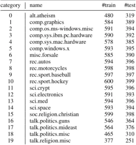
Table I: The filtered & vectorised20newsgroupsdataset.

category name #train #test

0 alt.atheism 480 319 1 comp.graphics 584 389 2 comp.os.ms-windows.misc 591 394 3 comp.sys.ibm.pc.hardware 590 392 4 comp.sys.mac.hardware 578 385 5 comp.windows.x 593 395 6 misc.forsale 585 390 7 rec.autos 594 396 8 rec.motorcycles 598 398 9 rec.sport.baseball 597 397 10 rec.sport.hockey 600 399 11 sci.crypt 595 396 12 sci.electronics 591 393 13 sci.med 594 396 14 sci.space 593 394 15 soc.religion.christian 599 398 16 talk.politics.guns 546 364 17 talk.politics.mideast 564 376 18 talk.politics.misc 465 310 19 talk.religion.misc 377 251 IV. EXPERIMENTS A. Dataset

We have conducted our experiments on a standard bench-mark dataset for text classification, 20newsgroups3. In order to ensure the reproducibility of our experimental results, we choose to use not the raw document collection, but a publicly-available ready-made “vectorised” version4. It has been split into training (60%) and testing (40%) subsets by date rather than randomly. Following the recommenda-tion of the provider, this dataset has also been “filtered” by striping newsgroup-related metadata (including headers, footers, and quotes). Therefore our reportedF1 scores will look substantially lower than those in the related literature, but such an experimental setting is much more realistic and meaningful. Table I shows the number of training documents and the number of testing documents for each category in this dataset.

B. Classifiers

In the experiments, we have applied our proposed ap-proach to carefully analyse the performances of two well-known supervised machine learning algorithms that are widely used for real-world text classification tasks: Naive Bayes (NB) and linear Support Vector Machine (SVM) [2]. For the former, we consider its two common variations: one with the Bernoulli event model (NBBern) and the other

with the Multinomial event model (NBM ult) [26], [27].

For the latter, we consider its two common variations: one with the L1 penalty (SVML1) and the other with the L2

penalty (SVML2) [28], [29]. Thus we have four different

classifiers in total. Obviously, the classification results of

3_{http://qwone.com/}∼_{jason/20Newsgroups/}

Table II: TheF1scores of the classifiers being compared. category NBBern NBM ult SVML1 SVML2

0 0.398 0.480 0.453 0.480 1 0.551 0.666 0.626 0.638 2 0.170 0.577 0.599 0.605 3 0.545 0.641 0.591 0.611 4 0.431 0.682 0.654 0.676 5 0.666 0.768 0.709 0.717 6 0.645 0.781 0.716 0.768 7 0.634 0.725 0.561 0.695 8 0.596 0.741 0.720 0.735 9 0.770 0.850 0.760 0.634 10 0.840 0.731 0.834 0.846 11 0.632 0.725 0.737 0.742 12 0.533 0.631 0.523 0.557 13 0.681 0.796 0.716 0.736 14 0.647 0.756 0.694 0.706 15 0.655 0.682 0.656 0.691 16 0.535 0.641 0.569 0.600 17 0.694 0.797 0.759 0.743 18 0.398 0.487 0.457 0.472 19 0.207 0.248 0.319 0.311 miF1 0.581 0.689 0.641 0.660 maF1 0.561 0.670 0.633 0.648

NBBern and NBM ultwould be highly correlated, and those

of SVML1 and SVML2 as well. Among them, SVML2 is widely regarded as the state-of-the-art text classifier [1], [4], [30]. It is also worth to notice that the NB algorithms will be applied not to the raw bag-of-words text datasets as people usually do, but on the vectorised 20newsgroups

dataset which has already been transformed by TF-IDF term weighting and document length normalisation.

We have used the off-the-shelf implementation of these classification algorithms provided by a Python machine learning libraryscikit-learn5in our experiments, again for the reproducibility reasons. The smoothing parameter α for the NB algorithm and the regularisation parameter C for the linear SVM algorithm have been tuned via grid search with 5-fold cross-validation on the training data for the macro-averagedF1score. The optimal parameters found are: NBBern with α = 10−14, NBM ult with α = 10−3,

SVML1 withC= 22, SVML2 withC= 21. C. Results

TheF1scores of these four classifiers in comparison, for each target category as well as the micro-average (miF1) and the macro-average (maF1), are shown in Table II. Please be reminded that the 20newsgroupsdataset used in our experiments is more challenging than most of its versions appeared in literature.

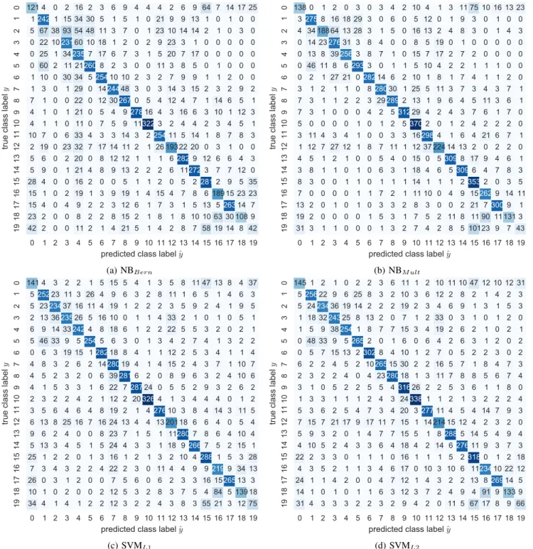
The confusion matrices of the classifiers provide all the data that our model needs to make comparison of averageF1 scores. They are shown in Fig. 3 to ensure the reproducibility of our experimental results.

5_{http://scikit-learn.org/stable/}

Table III: Frequentist comparison of the averageF1 scores. sign-test t-test NBBernvs NBM ult _mamiF_F1 0.000 0.000 1 0.000 0.000 SVML1 vs SVML2 _mamiF_F1 0.000 0.013 1 0.003 0.145 NBM ultvs SVML2 _mamiF_F1 0.000 0.000 1 0.115 0.138

Table III shows the results of frequentist comparison of the averageF1 scores. The column “sign-test” contains the two-sided p-values of using sign-test on the micro level (called s-test in [4]) and also the macro level (called S-test in [4]). The column “t-test” contains the two-sidedp-values of using unpaired t-test on the micro level (called p-test in [4]) and using pairedt-test on the macro level (called T-test in [4]). The above tests on the macro level are based on the classes’ F1 scores, but those on the micro level are actually based on the accuracy of document-class assignments which happens to be equivalent to miF1 in multi-class single-label (aka “one-of”) classification [2]. However, those tests will not longer be feasible on the micro level if we extend to multi-class multi-label (aka “any-of”) classification.

Table IV shows the results of Bayesian comparison of the average F1 scores, where the ROPE is set to [−0.005,+0.005]. It can be clearly seen that our proposed Bayesian approach offers a lot richer information about the difference between two classifiers’ average F1 scores than the frequentist approach does. In addition to the final judgement (“derision”) of comparison, we have shown the posterior “mean”, standard deviation (“std”), Monte Carlo error (“MC error”), the Bayes factor estimated by the SD method (“BFSD”), the percentage lower or greater than the

null value 0 (“LG pct”), the percentage covered by the ROPE (“ROPE pct”), and the 95% “HDI”. By contrast, the frequentist NHST based approach would lead to a far less complete picture as it has only the p-values (and maybe also the confidence intervals) to offer. Furthermore, note that the judgements made by the Bayesian estimation on several cases are different from those made by the frequentist NHST (e.g., at the significance level 5%). So even if in some researchers’ opinion the superiority of the former over the latter is still debatable, there is no doubt that the former can at least be complementary to the latter.

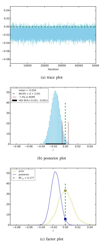
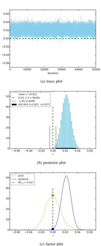
The Bayesian comparisons of maF1 for three pairs of text classifiers (NBBern vs NBM ult, SVML1 vs SVML2,

and NBM ult vs SVML2) are visualised in Fig. 4, 5, and

6 respectively. In each figure, the “trace plot” sub-graph shows the corresponding MCMC trace which proves the convergence of sampling; the “posterior plot” sub-graph shows the posterior probability distribution of the perfor-mance difference variable; and the “factor plot” sub-graph

0 1 2 3 4 5 6 7 8 9 10 11 12 13 14 15 16 17 18 19

predicted class label

ˆ

y

19 18 17 16 15 14 13 12 11 10 9 8 7 6 5 4 3 2 1 0

tru

e

cl

as

s

la

be

l

y

42 2 0 0 11 2 1 4 21 5 1 4 2 8 7 58 19 14 8 42 23 2 0 0 8 2 2 8 15 2 1 8 1 8 10 10 63 30 108 9 15 4 0 4 9 2 2 3 12 6 1 7 3 1 5 13 526314 7 15 1 0 2 19 1 3 9 19 1 4 15 4 7 8 6 189 15 23 23 28 4 0 0 16 2 0 0 5 1 1 2 0 5 22812 9 5 35 5 9 0 1 21 4 8 9 13 2 2 2 6 112723 7 7 12 0 5 6 0 2 20 0 8 12 12 1 1 1 62829 12 6 6 4 3 2 19 0 23 32 7 17 14 11 2 1 26 19322 20 0 3 1 0 0 10 7 0 6 33 4 3 3 14 3 225411 5 14 1 8 7 8 3 4 1 1 0 11 0 7 5 9 113223 2 4 4 2 3 4 5 1 4 1 0 1 21 0 5 4 927816 4 3 16 6 3 10 1 12 3 7 1 0 0 22 0 12 302670 5 4 12 4 7 1 14 6 5 1 1 3 0 1 29 0 1424448 3 0 3 14 3 15 2 3 2 9 2 1 10 0 30 34 525410 10 2 3 2 7 9 9 1 1 2 0 0 0 60 2 11 212608 2 3 0 0 11 3 8 5 0 1 0 0 0 0 25 1 342357 17 6 7 3 1 5 20 7 17 0 0 0 0 0 0 22 1023160 10 18 1 2 0 2 9 23 3 1 0 0 0 0 0 5 67 38 93 54 48 11 3 7 0 1 23 10 14 14 2 1 0 3 0 1242 1 15 34 30 5 1 5 1 0 21 9 9 13 1 0 1 0 0 121 4 0 2 16 2 3 6 9 4 4 4 2 6 9 64 7 14 17 25 (a) NBBern 0 1 2 3 4 5 6 7 8 9 10 11 12 13 14 15 16 17 18 19

predicted class label

ˆ

y

19 18 17 16 15 14 13 12 11 10 9 8 7 6 5 4 3 2 1 0

tru

e

cl

as

s

la

be

l

y

31 3 1 1 0 0 0 1 3 2 7 4 2 8 5 10123 9 7 43 19 2 0 0 0 0 1 5 3 1 7 5 2 11 8 11 90 11131 3 13 2 0 1 0 1 0 3 3 2 8 3 0 0 2 21 73009 1 7 0 0 0 0 1 1 7 2 1 11 10 0 4 9 152629 14 11 8 3 0 0 1 1 0 1 1 1 14 1 1 1 23532 0 3 5 3 8 1 1 0 1 0 6 3 1 18 4 6 53096 4 7 8 3 4 5 1 2 1 0 0 5 4 0 15 0 53098 17 9 4 6 1 1 12 7 27 12 1 8 7 11 1 12 37 224 14 13 2 0 2 2 0 3 11 4 3 4 1 0 0 3 3 162984 1 6 4 21 6 7 1 5 0 0 0 0 1 0 1 2 53702 0 1 2 4 2 2 2 0 7 3 1 0 0 0 4 2 531229 4 2 4 3 7 6 1 7 0 7 3 1 1 2 2 3 292892 13 1 9 6 4 5 11 3 6 1 3 1 2 1 1 0 828030 1 25 5 11 3 7 3 4 3 7 1 0 2 1 27 21 028214 6 2 10 1 8 1 7 4 1 1 2 0 0 46 11 8 62933 0 1 1 5 10 4 2 2 1 1 1 0 0 0 13 8 392563 8 7 1 0 15 7 17 2 7 2 0 0 0 0 0 14 2327631 3 8 4 0 0 8 5 19 0 1 0 0 0 0 0 4 34 18864 13 28 3 1 5 0 16 13 2 4 8 3 0 1 4 3 32758 16 18 29 3 0 6 0 5 12 0 1 9 3 0 1 0 0 138 0 1 2 0 3 0 3 4 2 10 4 1 3 11 75 10 16 13 23 (b) NBM ult 0 1 2 3 4 5 6 7 8 9 10 11 12 13 14 15 16 17 18 19

predicted class label

ˆ

y

19 18 17 16 15 14 13 12 11 10 9 8 7 6 5 4 3 2 1 0

tru

e

cl

as

s

la

be

l

y

34 4 1 4 1 2 2 12 3 2 2 4 3 8 3 55 21 3 12 75 10 1 0 2 0 0 2 12 5 3 2 8 3 7 5 4 84 5 139 18 26 0 3 1 2 0 0 7 5 6 0 6 2 3 3 16 1526513 3 7 3 4 3 2 2 4 22 2 3 0 11 4 4 9 92199 34 13 25 1 2 2 0 1 3 16 1 2 1 3 2 10 42881 5 3 28 5 13 3 4 5 1 5 24 4 3 3 1 18 92667 5 2 15 1 9 6 2 4 0 0 8 23 7 1 5 1 112807 8 6 4 10 4 6 13 8 25 16 7 16 24 13 4 4 13 20118 6 6 4 0 5 4 3 5 6 4 6 4 8 19 2 1 427610 3 8 4 14 3 11 5 2 3 2 2 4 2 1 12 2 203264 1 3 4 4 4 0 1 2 4 1 5 3 3 1 6 22 728724 0 5 5 2 9 3 2 6 2 4 5 2 3 2 0 6 392816 2 0 8 9 6 3 2 4 10 6 4 8 3 2 6 2 1428019 4 1 4 15 2 4 3 7 1 10 7 0 6 3 19 15 128218 8 4 1 1 12 2 5 3 4 1 1 4 5 46 33 9 52545 6 3 0 1 3 4 2 7 4 1 3 2 2 6 9 14 332424 8 18 6 1 2 2 22 5 5 3 2 0 2 1 2 13 3623526 5 16 10 0 1 1 4 33 2 1 0 1 0 5 1 5 2323437 16 11 4 19 1 2 2 2 3 5 9 2 4 1 9 5 525223 11 3 26 4 9 6 3 2 8 11 1 6 5 1 4 6 3 141 4 3 2 2 1 5 15 5 4 1 3 5 8 11 47 13 8 4 37 (c) SVML1 0 1 2 3 4 5 6 7 8 9 10 11 12 13 14 15 16 17 18 19

predicted class label

ˆ

y

19 18 17 16 15 14 13 12 11 10 9 8 7 6 5 4 3 2 1 0

tru

e

cl

as

s

la

be

l

y

31 4 3 3 3 2 2 3 2 9 4 2 0 11 5 67 17 8 9 66 14 1 0 1 0 1 1 6 3 12 3 7 2 4 9 4 91 9 133 9 24 1 1 4 2 0 0 4 7 12 1 4 3 2 2 13 826914 5 4 3 5 2 1 1 3 4 6 17 0 10 3 10 6 1123410 22 12 22 2 3 3 0 1 1 1 0 16 1 1 1 5 23180 1 2 18 4 10 5 2 4 3 3 6 4 18 4 2 14 627611 9 3 7 3 5 9 3 2 0 1 4 7 7 15 5 1 82885 14 5 4 9 4 7 15 7 21 17 9 17 11 7 15 1 14214 15 12 4 2 3 2 0 5 3 6 2 5 4 7 3 4 20 327711 4 5 4 14 7 9 3 1 3 3 1 1 1 2 4 3 243381 1 2 1 3 2 2 2 4 3 1 0 5 2 2 5 5 431626 2 2 5 3 6 1 1 8 0 2 3 2 2 4 0 4 2328018 1 3 11 7 8 8 5 6 7 4 6 2 2 4 5 2 1026515 30 2 2 16 5 7 1 8 4 7 3 0 5 7 15 13 23028 4 10 1 2 7 0 5 2 2 3 0 2 0 48 33 9 52652 0 1 6 0 6 4 2 6 3 1 2 0 2 1 5 9 382541 8 7 7 15 3 4 19 2 6 2 1 0 2 1 1 18 3224325 8 13 2 0 7 1 2 33 0 3 1 0 1 2 0 5 2423436 19 14 2 2 2 19 2 3 4 6 9 1 3 1 5 3 525622 9 6 25 8 3 2 10 3 6 12 2 8 2 1 4 2 3 145 1 2 1 0 2 2 3 6 11 1 2 10 11 10 47 12 10 12 31 (d) SVML2 Figure 3: The confusion matrices of the classifiers to be compared in our experiments.

shows the estimation of the Bayes factor by the SD method (see Section II-B1). The figures for miF1look very similar to those for maF1, so they are omitted due to the space limit. The results of our Bayesian comparison between NBBern

and NBM ult indicate that NBBern is significantly

outper-formed by NBM ult in terms of both miF1 and maF1. This confirms the finding of [26] on this harder dataset.

The results of our Bayesian comparison between SVML1 and SVML2 indicate that SVML1 is only slightly out-performed by SVML2 in terms of both miF1 and maF1 though the former may have its advantages sparsity. This is complementary to the findings reported in [28].

The results of our Bayesian comparison between NBM ult

Table IV: Bayesian comparison of the average F1scores.

mean std MC error BFSD LG pct ROPE pct HDI decision

NBBernvs NBM ult miF1 −0.107 0.008 0.000 0.000 100.0%<0<0.0% 0.0% [−0.122,−0.092] maF1 −0.109 0.008 0.000 0.000 100.0%<0<0.0% 0.0% [−0.123,−0.094] SVML1 vs SVML2 _mamiF_F1 −0.020 0.008 0.000 0.097 99.4%<0<0.6% 2.9% [−0.035,−0.005] < 1 −0.016 0.008 0.000 0.177 98.0%<0<2.0% 7.3% [−0.031,−0.001] < NBM ultvs SVML2 _mamiF_F1 +0.028 0.008 0.000 0.003 0.0%<0<100.0% 0.1% [+0.013,+0.043] 1 +0.022 0.008 0.000 0.027 0.2%<0<99.8% 1.3% [+0.007,+0.037]

and SVM camps — indicate that NBM ultworks a lot better

than SVML2 in terms of both miF1 and maF1, which is a bit surprising given that SVML2 is widely regarded as the state-of-the-art classifier for text classification. This some-what supports the claim of [31] that NBM ult, if properly

enhanced by TF-IDF term weighting and document length normalisation, can reach a similar or even better performance compared to SVML2.

V. EXTENSIONS

Our probabilistic model for comparing the average F1 scores has been described in the multi-class single-label (aka “one-of”) classification setting, but it is readily extensible to the multi-class multi-label (aka “any-of”) classification set-ting [1], [2]. In that case, the Dirichlet/Multinomial distribu-tions should simply be replaced by multiple Beta/Binomial distributions each of which corresponds to one specific target class, because a multi-class multi-label classifier is nothing more than a composition of independent binary classifiers.

To compare classifiers using a performance measure dif-ferent from the averageF1score (miF1or maF1), we would only need to replace the function f(µ,θ1, . . . ,θM) for

computing δ, as long as that performance measure could be calculated based on the classification confusion matrix alone. For example, it would be straightforward to extend our probabilistic model to handle the more generalFβ measure

(β≥0) withβ6= 1[2], [3].

In this paper we have focused on comparing text clas-sifiers, but our Bayesian estimation based approach can actually be used to compare classifiers on any type of data, e.g., images. Only the confusion matrices are needed for our models. It does not really matter what kind of data are classified.

VI. CONCLUSIONS

The main contribution of this paper is a Bayesian esti-mation approach to assessing the uncertainty of averageF1 scores in the context of multi-class text classification.

By modelling the full posterior probability distribution of miF1 or maF1, we are able to make meaningful interval estimation (e.g., the 95% HDI) instead of simplistic point estimationof a text classifier’s future performance on unseen data. The rich information provided by our model allows us to make much more comprehensive performance comparison

between text classifiers than what the traditional frequentist NHST can possibly offer.

REFERENCES

[1] F. Sebastiani, “Machine learning in automated text catego-rization,” ACM Computing Surveys (CSUR), vol. 34, no. 1, pp. 1–47, 2002.

[2] C. D. Manning, P. Raghavan, and H. Sch¨utze,Introduction to

Information Retrieval. Cambridge University Press, 2008.

[3] C. J. van Rijsbergen,Information Retrieval, 2nd ed. London, UK: Butterworths, 1979.

[4] Y. Yang and X. Liu, “A re-examination of text categorization methods,” in Proceedings of the 22nd Annual International ACM SIGIR Conference on Research and Development in

Information Retrieval (SIGIR), Berkeley, CA, USA, 1999, pp.

42–49.

[5] T. Mitchell,Machine Learning. McGraw Hill, 1997. [6] D. Zhang, J. Wang, and X. Zhao, “Estimating the uncertainty

of average F1 scores,” in Proceedings of the ACM SIGIR International Conference on Theory of Information Retrieval

(ICTIR), Northampton, MA, USA, 2015, in press.

[7] A. Gelman, J. Carlin, H. Stern, D. Dunson, A. Vehtari, and D. Rubin., Bayesian Data Analysis, 3rd ed. Chapman & Hall/CRC, 2013.

[8] J. K. Kruschke, Doing Bayesian Data Analysis: A Tutorial

with R, JAGS, and Stan, 2nd ed. Academic Press, 2014.

[9] ——, “Bayesian estimation supersedes the t test.”Journal of

Experimental Psychology: General, vol. 142, no. 2, p. 573,

2013.

[10] D. A. Hull, “Improving text retrieval for the routing problem using latent semantic indexing,” in Proceedings of the 17th Annual International ACM SIGIR Conference on Research

and Development in Information Retrieval (SIGIR), Dublin,

Ireland, 1994, pp. 282–291.

[11] H. Schutze, D. A. Hull, and J. O. Pedersen, “A comparison of classifiers and document representations for the routing problem,” in Proceedings of the 18th Annual International ACM SIGIR Conference on Research and Development in

Information Retrieval (SIGIR), Seattle, WA, USA, 1995, pp.

0 10000 20000 30000 40000 50000 iteration 0.12 0.10 0.08 0.06 0.04 0.02 0.00 δ

(a) trace plot

0.12 0.10 0.08 0.06 0.04 0.02 0.00 δ 0 10 20 30 40 50 mean = -0.109_{100.0% < 0 < 0.0%} 0.0% in ROPE HDI 95% [-0.123, -0.094] (b) posterior plot 0.12 0.10 0.08 0.06 0.04 0.02 0.00 δ 0 10 20 30 40 50 prior_posterior BFSD = 0.000 (c) factor plot

Figure 4: Comparing maF1 between NBBern and NBM ult.

[12] T. G. Dietterich, “Approximate statistical tests for comparing supervised classification learning algorithms,”Neural

Com-putation, vol. 10, no. 7, pp. 1895–1923, 1998.

[13] J. Demˇsar, “Statistical comparisons of classifiers over mul-tiple data sets,” The Journal of Machine Learning Research

(JMLR), vol. 7, pp. 1–30, 2006. 0 10000 20000 30000 40000 50000 iteration 0.08 0.06 0.04 0.02 0.00 0.02 0.04 δ

(a) trace plot

0.08 0.06 0.04 0.02 0.00 0.02 0.04 δ 0 10 20 30 40 50 mean = -0.016_{98.0% < 0 < 2.0%} 7.3% in ROPE HDI 95% [-0.031, -0.001] (b) posterior plot 0.08 0.06 0.04 0.02 0.00 0.02 0.04 δ 0 10 20 30 40 50 prior_posterior BFSD = 0.177 (c) factor plot

Figure 5: Comparing maF1 between SVML1 and SVML2.

[14] D. Barber, “Are two classifiers performing equally? a treat-ment using Bayesian hypothesis testing,” IDIAP, Tech. Rep., 2004.

[15] ——, Bayesian Reasoning and Machine Learning. Cam-bridge University Press, 2012.

0 10000 20000 30000 40000 50000 iteration 0.06 0.04 0.02 0.00 0.02 0.04 0.06 δ

(a) trace plot

0.06 0.04 0.02 0.00 0.02 0.04 0.06 δ 0 10 20 30 40 50 mean = +0.022_{0.2% < 0 < 99.8%} 1.3% in ROPE HDI 95% [+0.007, +0.037] (b) posterior plot 0.06 0.04 0.02 0.00 0.02 0.04 0.06 δ 0 10 20 30 40 50 prior_posterior BFSD = 0.027 (c) factor plot

Figure 6: Comparing maF1 between NBM ult and SVML2.

[16] J. N. Rouder, P. L. Speckman, D. Sun, R. D. Morey, and G. Iverson, “Bayesianttests for accepting and rejecting the null hypothesis,” Psychonomic Bulletin & Review, vol. 16, no. 2, pp. 225–237, 2009.

[17] Z. Dienes, “Bayesian versus orthodox statistics: Which side are you on?” Perspectives on Psychological Science, vol. 6,

no. 3, pp. 274–290, 2011.

[18] J. M. Dickey and B. P. Lientz, “The weighted likelihood ratio, sharp hypotheses about chances, the order of a markov chain,”

The Annals of Mathematical Statistics, vol. 41, no. 1, pp. 214–

226, 1970.

[19] R. Wetzels, J. G. Raaijmakers, E. Jakab, and E.-J. Wagen-makers, “How to quantify support for and against the null hypothesis: A flexible WinBUGS implementation of a default Bayesian t test,” Psychonomic Bulletin & Review, vol. 16, no. 4, pp. 752–760, 2009.

[20] E.-J. Wagenmakers, T. Lodewyckx, H. Kuriyal, and R. Gras-man, “Bayesian hypothesis testing for psychologists: A tu-torial on the Savage-Dickey method,”Cognitive Psychology, vol. 60, no. 3, pp. 158–189, 2010.

[21] C. Goutte and E. Gaussier, “A probabilistic interpretation of precision, recall andF-score, with implication for evaluation,”

in Proceedings of the 27th European Conference on IR

Research (ECIR), Santiago de Compostela, Spain, 2005, pp.

345–359.

[22] D. Koller and N. Friedman,Probabilistic Graphical Models

- Principles and Techniques. MIT Press, 2009.

[23] P. Resnik and E. Hardisty, “Gibbs sampling for the uniniti-ated,” Defense Technical Information Center (DTIC), Tech. Rep. LAMP-TR-153, 2010.

[24] D. J. C. MacKay,Information Theory, Inference, and

Learn-ing Algorithms. Cambridge University Press, 2003.

[25] A. Patil, D. Huard, and C. J. Fonnesbeck, “PyMC: Bayesian stochastic modelling in Python,” Journal of Statistical Soft-ware, vol. 35, no. 4, pp. 1–81, 2010.

[26] A. McCallum and K. Nigam, “A comparison of event models for Naive Bayes text classification,” in AAAI-98 Workshop

on Learning for Text Categorization, Madison, WI, 1998, pp.

41–48.

[27] V. Metsis, I. Androutsopoulos, and G. Paliouras, “Spam filter-ing with Naive Bayes - which Naive Bayes?” inProceedings

of the 3rd Conference on Email and Anti-Spam (CEAS),

Mountain View, CA, USA, 2006, pp. 27–28.

[28] J. Zhu, S. Rosset, T. Hastie, and R. Tibshirani, “1-norm support vector machines,” in Advances in Neural

Informa-tion Processing Systems (NIPS) 16, vol. 16, Vancouver and

Whistler, Canada, 2003, pp. 49–56.

[29] R.-E. Fan, K.-W. Chang, C.-J. Hsieh, X.-R. Wang, and C.-J. Lin, “LIBLINEAR: A library for large linear classification,”

Journal of Machine Learning Research, vol. 9, pp. 1871–

1874, 2008.

[30] D. D. Lewis, Y. Yang, T. G. Rose, and F. Li, “RCV1: A new benchmark collection for text categorization research,”

Journal of Machine Learning Research (JMLR), vol. 5, pp.

361–397, 2004.

[31] J. D. Rennie, L. Shih, J. Teevan, and D. R. Karger, “Tackling the poor assumptions of Naive Bayes text classifiers,” in Proceedings of the 20th International Conference on Machine