Modelling the short-term dependence between two
remaining lifetimes
Jaap Spreeuw and Xu Wang
March 27, 2008
Abstract
Dependence between remaining lifetimes in a couple is mainly of a short-term type if the mortality of the surviving member is highest in the first period after death of the partner. A multiple state model is introduced, allowing for this type of dependence, which is applied to a life annuity portfolio. The estimation results show that short-term dependence is clearly present and that the widowed lives feature an excess mortality, when compared to lives whose partner is still alive. Numerical illustrations involve the pricing, valuation and mortality profit analysis of contingent insurance contracts and reversionary annuities.
1
Introduction
Traditionally, it has been presumed in multiple life contingencies that the remaining life-times of the lives involved are mutually independent. As some empirical investigations have shown, for coupled lives, this standard assumption is based on computational con-venience rather than realism.
Over the past few years, several papers about insurance contracts on two lives have been published which allow for dependence between the two lifetimes. Frees et al. (1996) and Carriere (2000) present alternative ways of modeling dependence of times of death of coupled lives and applying them to a data set. In both papers, a significant degree of positive correlation between lifetimes is observed. This implies, for instance, that joint life annuities are underpriced while last survivor annuities are overpriced. Carriere and Chan (1986) present boundaries of single premiums for last survivor annuities. All three papers adopt a methodology based on copulas, an approach which is popular nowadays.
Frees et al. (1996) also use common shock models as an alternative way of specifying dependence. Common shock models have been introduced by Marshall and Olkin (1967, 1988). Such models, however, do not fit their data as well as their copula model.
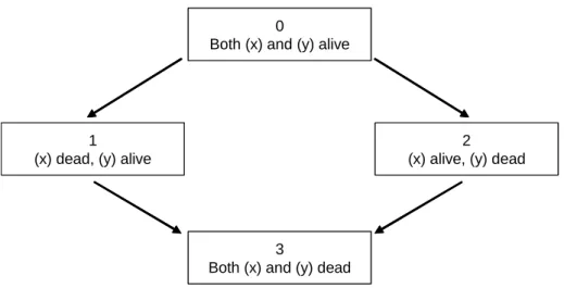
Norberg (1989) and Wolthuis (2003) design a basic, time-continuous Markov chain for the mortality status of a couple. This model is depicted in Figure 1.
In this model, µ01(·) and µ23(·) are the forces of mortality for a man whose partner
is still alive and a man whose partner has died, respectively. Likewise, µ02(·) andµ13(·)
represent the respective forces of mortality for a woman whose spouse is still alive and a woman whose spouse has died. As shown in Norberg (1989), the dependence between the
0
Both (x) and (y) alive
3
Both (x) and (y) dead 1
(x) dead, (y) alive
2 (x) alive, (y) dead 0
Both (x) and (y) alive
3
Both (x) and (y) dead 1
(x) dead, (y) alive
2 (x) alive, (y) dead
Figure 1: Markov model as in Norberg (1989) and Wolthuis (2003)
two remaining lifetimes follows from the inequality between the forces of mortalityµ01(·)
and µ23(·), as well as µ02(·) and µ13(·). Wolthuis (2003) assumes a simple parametric specification of the forces of mortality as a function of a baseline force of mortality, using one parameter for dependence only. Denuit and Cornet (1999) generalize Wolthuis’ approach by allowing for four parameters, one parameter per type of transition intensity, see also Denuit et al. (2001). Applying the model to a Belgian data set, they establish a significant reduction in the mortality of married men and women, and a significant increase in the mortality of widows and widowers, compared to average lives from the Belgian population.
All these papers study the impact of dependence of two remaining lifetimes on the pricing of life insurance products on the lives concerned.
Dependence, however, also affects the valuation of such contracts over time. Prospec-tive provisions are based on laws of mortality that apply to the policy valuation date. If the remaining lifetimes of a couple are dependent at the outset of a policy, then any of the two lives’ survival probabilities may depend on the life status of the partner.
Moreover, it is not sufficient just to conclude that there is dependence between re-maining lifetimes. It is also essential to state what type of dependence applies. Hougaard (2000) points out that within a time framework, one can basically distinguish between three different categories:
1. Instantaneous dependence: dependence caused by common events affecting both lives at the same time.
2. Long-term dependence: dependence which is caused by a common risk environment, affecting the surviving partner for their remaining lifetime.
3. Short-term dependence: the event of death of one life changes the mortality of the other life immediately, but this effect diminishes over time.
Instantaneous dependence is implied due to the fact that both members of a couple are prone to common events such as accidents. Dependence is assumed to be of a long-term nature if the force of mortality of the survivor is a constant or increasing function
of the time of death of the partner. On the other hand, dependence is taken to be short-term if this force of mortality is a decreasing function of the time of death of the partner. An example of long-term dependence is the mechanism of matching couples (“birds of a featherflock together”). For instance, two partners often come from the same neighbourhood which determines their common risks. The “broken heart syndrome” (as researched in Parkes et al., 1969, and Jagger and Sutton, 1991) is the most well-known example of short-term dependence.
It is a question which type of dependence prevails within the framework of multiple life contingencies. Hougaard (2000) suggests that in case of a married couple, short-term dependence is perhaps more relevant than long-short-term dependence. This assertion is underpinned by one of the main results from the empirical work in Parkes et al. (1969) and Jagger and Sutton (1991). Both studies show that within about 6 months after death of the partner, the mortality of widowers is comparable with that of married men.
Spreeuw (2006) has shown that most common Archimedean copulas exhibit long-term dependence. This includes all copulas with a frailty specification such as Frank (used in Frees et al., 1996), Clayton, and Gumbel Hougaard. Youn and Shemyakin (1999, 2001) show that, when implementing a copula model, ignoring the difference between the physical ages of the two partners can lead to an underestimation of the instantaneous dependence and short-term dependence. Shemyakin and Youn (2006) adopt a Bayesian approach, allowing for incorporation of prior knowledge about individual mortality.
Jagger and Sutton (1991) apply the Cox proportional hazard model (for details, see Cox, 1972) to a small data set, where apart from age, other risk factors such as physical disability, physical impairment, and cognitive impairment are used as covariates. The basic Markov model, as applied in Denuit and Cornet (1999) is a special case of long-term dependence, since the mortality of a remaining life is independent of the time of death of the spouse.
In this paper, we will use an extended Markov model allowing mortality of a remaining life to depend on the time elapsed since death of the spouse. Upon death of the spouse, each widow(er) will first enter an initial state and stay there for a limited period, or until death. If at the end of this period the life is still alive, it enters a next state, from which only a transition to the Death state can be made. The crucial point is that the survivor’s mortality in this ultimate state is allowed to differ from that in the initial state (entered immediately on death of the spouse). Such a model allows explicitly for short-term dependence. We will apply this model to the same data set as used in Frees et al. (1996), Carriere (2000), Youn and Shemyakin (1999, 2001) and Shemyakin and Youn (2006).
Using this extended Markov model, we study the impact on premiums and provisions of some policies that remain in force after death of one specific life.
In Section 2, we give proper definitions of long-term dependence and short-term de-pendence, as derived in Spreeuw (2006). Section 3 gives the main characteristics of the data set and makes the case for developing models for short-term dependence. Section 4 introduces the extended Markov model and shows the estimation method, analogous to Denuit et al. (2001). Section 5 gives the results of the estimation. In Section 6, we show the impact on the pricing and valuation of policies over time. We also demonstrate the impact on variability of the mortality profit arising in the year just after death of one of the lives. Section 7 sets out a conclusion.
2
Types of dependence
We consider two lives(x)and(y), agedxandy, respectively at duration0. The complete remaining lifetimes of(x)and(y)are denoted byTx andTy, respectively. We assume that
TxandTy are continuously distributed, with upper boundsωx−xandωy−y, respectively.
The variables ωx andωy denote the limiting ages of (x) and(y). For t∈ [0, ωx−x)and
s ∈ [0, ωy−y), we define µ1(x+t) and µ2(y+s) as the forces of mortality relating to
Tx andTy.
Defineµ1(x+t|Ty =ty)as the conditional force of mortality of(x)at durationt(age
x+t) given that(y)has died at durationty (agey+ty) withty ∈[0, t). Likewise, we define
µ2(y+s|Tx =tx) as the conditional force of mortality of (y) at duration s (age x+s)
given that(x)has died at durationtx (agey+tx) withtx ∈[0, s). Now we can specify the
notion of long-term and short-term dependence, using the definition in Spreeuw (2006).
Definition 1 The remaining lifetimes Tx and Ty exhibit short-term dependence if
µ1(x+t|Ty =ty)is an increasing function ofty ∈[0, t](or alternatively, ifµ2(y+s|Tx =tx)
is an increasing function oftx ∈[0, s]). On the other hand, there is long-term dependence
betweenTx andTy ifµ1(x+t|Ty =ty)is constant or decreasing as a function ofty ∈[0, t]
(or equivalently, ifµ2(y+s|Tx =tx)is constant or decreasing as a function oftx ∈[0, s]).
3
The data set
We use the same data set as Frees et al. (1996), Carriere (2000) and Youn and Shemyakin (1999, 2001) and Shemyakin and Youn (2006). The original data set concerns 14,947 contracts in force with a large Canadian insurer. The period of observation runs from December 29, 1988, until December 31, 1993. Like the aforementioned papers, we have eliminated same-sex contracts (58 in total). Besides, like Youn and Shemyakin (1999, 2001), for couples with more than one policy, we have eliminated all but one contracts (3,435 contracts). This has left us with a set of 11,454 couples or contracts, which can be broken down in four sets, according to the survival status at the end of the observation. There were 195 couples where both lives died during the observation period, 1,048 couples where the male died and the female survived during the period, 255 couples where the female died and the male survived, and 9,956 couples where both survived. For the ease of wording, in the remainder of this paper we will assume that all couples are married couples. What matters is that the coupled lives have a permanent relationship. The question whether or not each relationship is a marital type is of secondary importance.
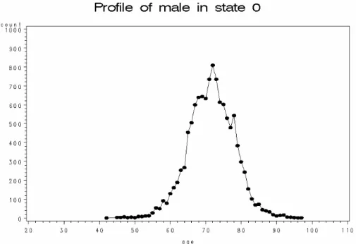
To give an impression of the age groups concerned, we first give a distribution of the ages of the lives at the start of the observation. Figures 2 and 3 display these distributions for males and females, respectively.
As there were not many couples in the data set with at least one of the lives aged 40 or below, it was decided to leave them out (88 in total).
Next, in order to illustrate our case, we analyse the data in aggregate format. Wefirst combine the widows and widowers into one group, and then split them up according to a variable e, denoting the number of years elapsed since the death of the partner. We use the label “Elapse e”, to indicate that the spouse died betweene ande+ 1 years ago. We have e ∈{0, ..,4}. For each of the five groups, we calculate the Risk Exposure, in years,
Figure 2: Profile of male in state 0 at entry
Elapse e Deaths Exposure Mortality 0 126 1,230.64 0.102389 1 35 869.18 0.040277 2 18 551.58 0.032633 3 8 312.66 0.02559 4 6 106.25 0.05647 Partner alive 1,410 83,738.58 0.016838
Table 1: All group mortality
Age e=0 e=1 e=2 e=3 e=4 Partner alive Ratio e=0
e=1 65 0.0139 0.0204 0.0068 0.0123 0.0000 0.0027 0.6790 70 0.0295 0.0321 0.0223 0.0163 0.0226 0.0057 0.9194 75 0.0698 0.0366 0.0363 0.0180 0.0257 0.0132 1.9058 80 0.1221 0.0146 0.0653 0.0351 0.0000 0.0313 8.3678 85 0.1586 0.0508 0.1093 0.0849 0.0000 0.0227 3.1233 90 0.1954 0.1713 0.0688 0.0806 0.0000 0.0413 1.1407
Table 2: Mortality of widows as a function of time elapsed since death of spouse and derive the observed number of deaths. Then, naturally, the mortality follows as the ratio between the two. The results are shown in Table 1.
From these numbers, we can clearly see that:
• the mortality for widows and widowers is higher than for lives whose partner is still alive;
• the mortality is highest among lives who have lost their partner recently, i.e. less than one year ago.
The following step concerns distinguishing between the sexes and allowing for the impact of age.
By building on the approach adopted in the previous paragraph, we analyse the mor-tality of widows and widowers separately, depending on the time elapsed since death of the partner, and compare this with the mortality experienced by married couples. Ide-ally, we would calculate estimates of widow(er)s mortality for a certain age, according to the exposed to risk and number of deaths observed for that age. Due to a lack of data, however, we will estimate mortality as a 9 year moving average basis. For instance, the estimated rate of mortality for a widow aged 65 with e = 1 is calculated by taking the total number of deaths of widows observed between ages 61 and 70 exact whose partner died between1 and2 years ago. For the same age interval, we derive the exposed to risk. These mortality rates are derived for e ∈ {0, ..,4} and will be compared with those of a man or woman of the same age, whose partner is still alive. Tables 2 and 3 show the mortality of widows and widowers, respectively, forx= 65 + 5i, i∈{0, ..,5}.
Age e=0 e=1 e=2 e=3 e=4 Partner alive Ratio ee=0=1 65 0.1739 0.0338 0.0634 0.0000 0.0000 0.0113 5.1417 70 0.1835 0.0695 0.0254 0.0556 0.0000 0.0194 2.6423 75 0.1749 0.0693 0.0000 0.0285 0.0000 0.0310 2.5248 80 0.4699 0.0923 0.0461 0.0000 0.2322 0.0553 5.0891 85 0.6206 0.1092 0.1219 0.0000 0.2830 0.0968 5.6850 90 0.5097 0.1452 0.0888 0.2150 0.3785 0.0703 3.5088
Table 3: Mortality of widowers as a function of time elapsed since death of spouse • The lack of data is a significant problem. For both tables, there are some cells where
zero deaths have been observed, and hence the estimated rate of mortality is also equal to zero. Furthermore, in some columns, contrary to what one would expect, the mortality is not always increasing as a function of age.
• In the majority of the cases, the mortality of widow(er)s is significantly higher than that of lives whose partner is still alive. This would imply a strong dependence between the lifetimes of coupled lives (as confirmed in previous studies).
• In most cases, the mortality of widow(er)s whose partner died less than a year ago is higher than the mortality of other widow(er)s. The mortality of lives whose partner died more than a year ago shows an irregular pattern as a function of e.
• The last column shows the ratio of the mortality of widowed lives whose partner died less than a year ago to the mortality of widowed lives whose partner died between one and two years ago. With one exception, this ratio is higher for widowers than for widows. This seems to suggest that the broken heart syndrome has a stronger impact on men than on women.
4
The Markov model extended
4.1
Presenting the model
Before presenting our model, we first deal with the model by Denuit and Cornet (1999). Using the model by Norberg (1989) and Wolthuis (2003), as depicted in Figure 1, Denuit and Cornet specified the following conditional forces of mortality as a function of the marginal forces of mortality:
µ01(t) = µ1(x+t|Ty > t) = (1−α∗01)µ1(x+t) ;
µ02(t) = µ2(y+t|Tx > t) = (1−α∗02)µ2(y+t) ;
µ13(t) = µ2(y+t|Tx ≤t) = (1 +α∗13)µ2(y+t) ;
µ23(t) = µ1(x+t|Ty ≤t) = (1 +α∗23)µ1(x+t) ;
α∗01, α∗02, α∗13, α∗23 ≥ 0.
Note that in this model, death of the man leads to a constant increase of the woman’s mortality by 1+α∗13
1−α∗
02, and that a man’s mortality goes up by a factor
1+α∗ 23
1−α∗
0
Both (x) and (y) alive
1
(x) dead, (y) alive 0 <= time since (x) died < t1
5
Both (x) and (y) dead 2
(x) dead, (y) alive time since x died >= t1
3
(x) alive, (y) dead 0 <= time since (y) died < t2
4
(x) alive, (y) dead time since (y) died >= t2 0
Both (x) and (y) alive
1
(x) dead, (y) alive 0 <= time since (x) died < t1
5
Both (x) and (y) dead 2
(x) dead, (y) alive time since x died >= t1
3
(x) alive, (y) dead 0 <= time since (y) died < t2
4
(x) alive, (y) dead time since (y) died >= t2
Figure 4: Six-state model
spouse dies. Note as well that this model is a special case of long-term dependence, since the mortality of one life only depends on whether the spouse has died or not, and not when (s)he died.
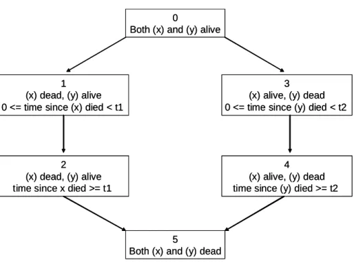
We allow for short-term dependence by adding two states, one for the widow and one for the widower. This leads to a six-state model as shown in Figure 4.
A woman getting widowed will enter the state1 ((y)alive, (x)died less thant1 years
ago) in which she will stay for at most t1 years, after which, if still alive, she makes the
transition to state 2 ((y) alive, (x) died more than t1 years ago) from which only the
transition to state 5 (Both dead) is possible. Likewise, a man losing his spouse willfirst enter state 3 ((x) alive, (y) died less than t2 years ago) where he will stay for at most
t2 years, after which he will automatically make the transition to state 4 and stay there
while alive. Note that t1 and t2 do not need to be the same! This allows for a different
type of broken heart effect for males and females.
Using the extended model in a proportional hazards setting requires additional para-meters. The specification is:
µ01(t) = µ1(x+t|Ty > t) = (1−α01)µ1(x+t) ; µ03(t) = µ2(y+t|Tx > t) = (1−α03)µ2(y+t) ; µ15(t) = µ2(y+t|0≤t−Tx < t1) = (1 +α15)µ2(y+t) ; µ25(t) = µ2(y+t|t−Tx ≥t1) = (1 +α25)µ2(y+t) ; µ35(t) = µ1(x+t|0≤t−Ty < t2) = (1 +α35)µ1(x+t) ; µ45(t) = µ1(x+t|t−Ty ≥t2) = (1 +α45)µ1(x+t) ; α01, α03, α15, α25, α35, α45 ≥ 0.
Figure 5: Profile of age of widow on entering state 1.
α35=α45=α∗23. Inequalities between the parameters reflect the main type of dependence
between lifetimes.
4.2
Application to data set
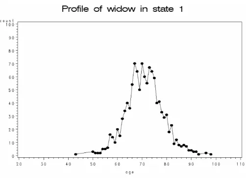
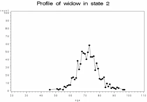
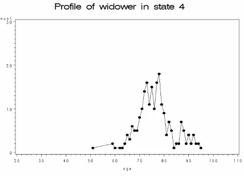
For t1 = 1 andt2 = 1, a profile of the age upon entering the several widow(er)’s states is
given in the Figures 5 to 8.
Note that a drawback of this model is the jump in mortality experienced by the transition from state 1 to 2, and from state 3 to 4. Ideally, we should adopt a semi-Markov model, which allows the mortality of the widow(er) to be a continuous function of time elapsed since death of the spouse. However, such non-homogeneous Semi-Markov models, where the transition intensity depends on age as well, require a lot of data. It is for this reason that we use this model instead, which is in fact a Markov model with splitting of states. This methodology has also been applied for the purpose of estimating rates of recovery from disability. These rates have shown to depend strongly on the duration of sickness. The methodology has been described in Haberman and Pitacco (1999). For an application, see Gregorius (1993). Another application of duration dependence in Markov chains concerns select mortality, see Norberg (1988) and Möller (1990).
We note from the Figures 5 to 8 that the availability of data is a serious problem. This is due to the fact that the number of widows and, in particular, widowers is small. In the next section, we will see that the standard errors of estimates pertaining to widowers are quite high.
Figure 6: Profile of age of widow on entering state 2 fort1 = 1.
Figure 8: Profile of age of widower on entering state 4 fort2 = 1.
5
Estimation
5.1
Methodology
Like Frees et al. (1996) and Carriere (2000), we have specified the marginal forces of mortality function to be Gompertz. This implies:
µx = 1 σm ex−σmmm;µy = 1 σf e y−mf σf (1)
Just as in Frees et al., and Carriere, estimation of the parameters has been done by Maximum Likelihood. This leads to the estimates mm = 86.37;σm = 9.76;mf =
92.07;σf = 8.06. We note slight discrepancies inσ values compared to Frees et al. (1996)
and Carriere (2000). This may be due to our data set being slightly different from the one used in the aforementioned papers.
Given these values, we estimate the parameters α by maximum likelihood. For lives in state 0, this leads to estimates of the type
b α01= 1− d01 P i:all males RExitAge(i) EntryAge(i)µxidxi ;αb02 = 1− d02 P i:all females RExitAge(i) EntryAge(i)µyidyi , (2)
where d01 (d02) is the observed number of male (female) deaths in state 0. We see from
(2) that for each life under risk we take the force of mortality with parameters estimated as above, integrated over the age range in which the life was under observation. Note that the observation ends at death or censoring. The standard errors are obtained by the
t1 = 0.5 andt2 = 0.5 α01 α15 α25 α03 α35 α45 Estimate 0.06 5.06 1.24 0.14 13.27 0.38 Number of deaths 840 27 39 266 51 20 Standard error 0.037 1.17 0.36 0.07 2.00 0.31 t1 = 1 andt2 = 1 Estimate 0.06 3.40 1.15 0.14 7.19 0.41 Number of deaths 840 37 29 266 55 16 Standard error 0.037 0.72 0.40 0.07 1.10 0.35 t1 = 1.5 andt2 = 1.5 Estimate 0.06 2.84 1.06 0.14 5.47 0.06 Number of deaths 840 45 21 266 62 9 Standard error 0.037 0.57 0.45 0.07 0.82 0.35
t1 =∞and t2 =∞(four-state model)
Estimate 0.06 2.01 N/A 0.14 2.93 N/A
Number of deaths 840 66 N/A 266 71 N/A
Standard error 0.037 0.371 N/A 0.07 0.47 N/A Table 4: Estimates of parameters of dependence
formula s.e.[bα0j] = 1−bα0j p d0j ; j ∈{1,2}.
For lives in states 1, ..,4, we get as estimates: b αj5 = dj5 S i:a ll fe m a le s in sta tej UExitAge(i) EntryAge(i)µyidyi − 1; j ∈{1,2} b αk5 = S dk5 i:a ll m a le s in s ta tej UExitAge(i) EntryAge(i)µxidxi − 1; k ∈{3,4} . (3)
Note that for each life exposed, we integrate the baseline force of mortality from the entry age to the exit age. The standard errors of the estimates in (3) are specified as
s.e.[bαj5] =
1 +bαj5
p
dj5
; j ∈{1, ..,4}.
The estimates have shown to be very sensitive to the choice of age range. In estimating these coefficientsbαj5, we used as ages of entry the intervals[65,85]for males and[60,80]for
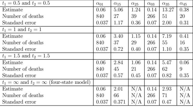
females, as these intervals contain the largest proportion of widowed lives. Our findings also suggest that the dependence between the two lifetimes depends on the ages. For several values of t1 andt2, the results are as shown in Table 4.
This table clearly shows that α01 is smaller than both α15 and α25. Similarly, α03
is smaller than both α35 and α45. This implies that the lifetimes are clearly dependent
on each other. The table also shows that α15 < α25, as well as that α35 < α45. This
suggests short-term dependence for both genders, for widowers stronger than for widows. However, the estimates of the coefficients α15, .., α45 all have quite large standard errors,
so care must be taken before drawing any firm conclusions.
The last four rows display the parameters pertaining to the standard four-state Markov model as in Figure 1. Note that t1 =∞ andt2 =∞ implyα15=α∗13 andα35=α∗23, and
As argued above, there is only a small number of widowers, and therefore the estimates do not seem to be very reliable. For this reason, the calculations and results in the reminder of this paper will be given for widows only.
5.2
Testing the model on short-term dependence
We have seen in the previous paragraphs that there are significant differences between the parameters α15 and α25, and also between α35 andα45. However, the number of widows
and widowers is small, so the difference could be due to chance.
In this paragraph, we test whether widower’s mortality depends significantly on the time elapsed since death of the spouse. This means that we test the null hypothesis
H0 :α15=α25,
against the alternative hypothesis
H1 :α156=α25.
If H0 is true, then the observed mortality rates in states 1 and 2 are two samples from
the same survival function, otherwise they are governed by different survival functions. Thus, our test can be transformed to:
H0 : S(y)15(t) =S(y)25(t)
H1 : S(y)15(t)6=S(y)25(t),
where S(y)i5(t) is the survival function of a widow agedy in statei, i∈{1,2}.
Following Kolmogorov-Smirnov test for two samples, we compute
Dmn = sup t ¯ ¯S(y)m(t)−S(y)n(t) ¯ ¯,
where S(y)m(t) is the Kaplan Meier function corresponding to S(y)15(t) and m deaths.
Likewise, S(y)n(t) denotes the Kaplan Meier function corresponding to S(y)15(t) and n
deaths. The null hypothesis is rejected when µ mn m+n ¶1 2 Dmn ≥c,
where c is the critical value of the Kolmogorov distribution given a certain significant level. For y= 60, the results are shown in Table 5, where we define b=¡mmn+n¢
1 2 D
mn.
We note that the highert1, the higher thep-value. For t1 = 0.5 or t1 = 1, the test is
significant at 5% level, but not for higher t1.
So it seems that botht1 = 0.5ort1 = 1are suitable as cut-offpoints between the states
1 and 2. For computational convenience, we chooset1 = 1 in the numerical examples in
the next Section.
Note that a similar test could be undertaken for widower’s mortality (comparingα35
t1 0.5 1 1.5 2 2.5 Dmn 0.4355 0.3205 0.2446 0.2456 0.1590 m 34 48 58 66 70 n 52 38 28 20 16 b 1.9755 1.4759 1.0631 0.9622 0.5739 p-value 0.0009 0.0259 0.209 0.3134 0.8948
Table 5: Outcomes of Kolmogorov Smirnov test
6
Impact on premiums and provisions
Given our estimates in the previous section, we now analyse the impact of the type of dependence on the pricing and valuation of contracts which may still be in force when one of the lives dies. We have chosen the following contracts, both of a whole life type:
• Contingent assurance contracts: a benefit of1 is payable immediately on the death of (y), provided this happens after the death of (x). We distinguish between the following three premium payment arrangements: a) single premium payment; b) level premium payment annually in advance while both alive (referred to as Level Premium I), and c) level premium payment annually in advance while (y) alive (referred to as Level Premium II).
• Reversionary annuities: a benefit of 1 p.a. is payable in arrears, starting at the end of the year of (x)’s death, and continuing while (y) survives. We distinguish between: a) single premium payment, and b) level premium payment annually in advance while both alive.
For both types of contracts, we:
• calculate the premium payable, under several premium payment arrangements; • calculate the state-dependent net premium provisions at several durations. When
calculating provisions in state 0, i.e. both lives are alive, we calculate the value at 0, 1, 5, 10, 15, 20 years since the start of the contract. When calculating provisions in State 1 (or 2), i.e. the male has died and the female is still alive, the time of death of the male can take the values 15, 19.25, 19.5, 19.75 and 20 years (all from the start of the contract) while the provision is calculated at dates 20, 20.25, 20.5, 20.75, 21, 25 and 30.
• analyse the variability of the mortality profit in year starting on death of the spouse. In our calculations, we distinguish between three models:
1. Model A: Independence of the remaining lifetimesTx and Ty.
2. Model B: the classical four-state model as developed in Denuit and Cornet (1999), as displayed in Figure 1. The mortality of widow(er)s does not depend on time elapsed since death of the spouse. This impliesα∗
13=α15 =α25andα∗23=α35=α45. Using
Model A Model B Model C
Single premium payment 0.114 0.151 0.142
Level Premium I 0.008 0.010 0.010
Level Premium II 0.007 0.009 0.009
Table 6: Premiums for contingent assurance
Time Single Premium Level premium I Level premium II
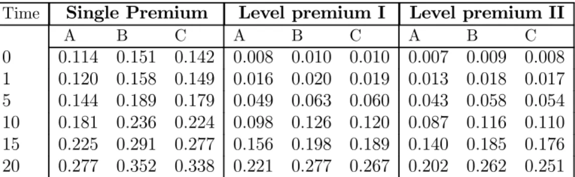
A B C A B C A B C 0 0.114 0.151 0.142 0.008 0.010 0.010 0.007 0.009 0.008 1 0.120 0.158 0.149 0.016 0.020 0.019 0.013 0.018 0.017 5 0.144 0.189 0.179 0.049 0.063 0.060 0.043 0.058 0.054 10 0.181 0.236 0.224 0.098 0.126 0.120 0.087 0.116 0.110 15 0.225 0.291 0.277 0.156 0.198 0.189 0.140 0.185 0.176 20 0.277 0.352 0.338 0.221 0.277 0.267 0.202 0.262 0.251
Table 7: Provisions in state 0 for the contingent assurance
3. Model C: the model allowing the mortality of widow(er)s to depend on time elapsed since death of the spouse. For t1 = 1 and t2 = 1, we use the estimates bα01 =
0.06;αb03 = 0.14 (obviously, for lives with partner alive, the estimates are the same
as in Model B), and further αb15 = 3.40;αb25= 1.15;bα35 = 7.19;αb45= 0.41.
For both policies, we take as ages at issue x = 55 and y = 50. Interest is at 5% per annum.
6.1
Contingent assurance contracts
6.1.1 Premiums
The premiums are tabulated in Table 6.
We notice, for the purposes of both premium and provision calculations, that Model C gives values which are between the values for Model A and Model B. Here, Model B results in the highest premiums, followed by Model C and Model A. Dependence causes premiums for contingent assurances to be higher; this is why Model A gives the lowest premiums. The lower premium for Model C is due to the lower mortality experienced by widows after a year. Apparently, this effect outweighs the impact of higher mortality in the first year after getting widowed.
6.1.2 Provisions
Table 7 gives the provisions in state 0 for contingent assurances. Note again that Model B gives the highest values, and Model A the lowest values.
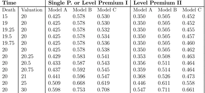
In Table 8, we can view the provisions to be held at several durations when(x)has died and(y)is still alive. Obviously, death of the male causes the payment of the sum assured to be made with certainty. This is why the provisions in this Table are significantly higher than the values in Table 7.
Time Single P. or Level Premium I Level Premium II
Death Valuation Model A Model B Model C Model A Model B Model C
15 20 0.425 0.578 0.530 0.350 0.505 0.452 19 20 0.425 0.578 0.530 0.350 0.505 0.452 19.25 20 0.425 0.578 0.532 0.350 0.505 0.455 19.5 20 0.425 0.578 0.534 0.350 0.505 0.457 19.75 20 0.425 0.578 0.536 0.350 0.505 0.460 20 20 0.425 0.578 0.538 0.350 0.505 0.462 20 20.25 0.429 0.583 0.541 0.353 0.508 0.463 20 20.5 0.433 0.587 0.543 0.356 0.511 0.464 20 20.75 0.437 0.592 0.545 0.359 0.514 0.464 20 21 0.441 0.596 0.547 0.368 0.526 0.473 20 25 0.509 0.668 0.619 0.446 0.611 0.558 20 30 0.598 0.753 0.708 0.547 0.711 0.661
Table 8: Provisions in state 1 or 2 (Model C) or state 1 (Model B) for the contingent assurance contract
The provision at duration 20 has been tabulated according to different periods elapsed since death of the spouse, i.e. spouse died 1 year ago (duration 19), 9 months ago (duration 19.25), half a year ago (duration 19.5), 3 months ago (duration 19.75), or has just died (duration 20). Model C allows for these differences and gives the highest values for death at duration 20 (due to the short-term dependence). Note that Model B does not take account of any time elapsed since death of the partner. Therefore, the provision is fixed at 0.5784.
Further in the table, provisions have been tabulated, where the time of death of the spouse is fixed (at 20), but the contract has been valued at various durations (20, 20.25, 20.5, 20.75, 21, 25 and 30). In this case, the provisions go up with duration for all models. Obviously the premium payment arrangements of Single Premium and Level Premium I lead to the same provision (since in both cases, no premiums are payable after (x)’s death).
6.1.3 Mortality profit
In our model, the mortality of those who got bereaved recently is highest. In this section, we analyse the impact of this feature on the mortality profit. For several policy years, the Death Strain at Risk, the Expected Death Strain, and the Standard Deviation of the mortality profit are given, where it is assumed that the first death occurred at the end of the previous year.
For a sum assured of 1, the standard deviation of the mortality profit per policy in policy year (t, t+ 1] in Model k, denoted by SDtk, is calculated as
SDkt = q qk y+t ¡ 1−qk y+t ¢ DSARkt,
where k indicates the model used,k ∈{A, B, C} and
Duration DSAR EDS S.D. of MP A B C A B C A B C 0 0.810 0.718 0.750 0.001 0.002 0.002 0.022 0.033 0.042 5 0.762 0.653 0.690 0.001 0.003 0.004 0.028 0.041 0.053 10 0.705 0.577 0.619 0.002 0.004 0.007 0.035 0.050 0.064 15 0.637 0.493 0.540 0.003 0.007 0.011 0.043 0.057 0.076 20 0.559 0.404 0.453 0.005 0.010 0.017 0.051 0.064 0.085 25 0.473 0.314 0.363 0.007 0.015 0.024 0.059 0.066 0.091 30 0.384 0.231 0.275 0.011 0.020 0.034 0.065 0.065 0.090
Table 9: Death Strain at Risk (DSAR), Expected Death Strain (EDS), and Standard Deviation (S.D.) of mortality profit (MP) for a contingent assurance; Single Premium Payment and Level Premium Payment I
Duration DSAR EDS S.D. of MP
A B C A B C A B C 0 0.917 0.847 0.875 0.001 0.002 0.003 0.025 0.039 0.049 5 0.862 0.769 0.805 0.001 0.003 0.005 0.031 0.049 0.061 10 0.797 0.679 0.722 0.002 0.005 0.008 0.040 0.058 0.075 15 0.720 0.580 0.629 0.003 0.008 0.013 0.049 0.068 0.088 20 0.632 0.474 0.527 0.005 0.012 0.019 0.058 0.075 0.099 25 0.534 0.368 0.421 0.008 0.017 0.028 0.067 0.078 0.106 30 0.433 0.270 0.319 0.013 0.023 0.039 0.073 0.075 0.104
Table 10: Death Strain at Risk (DSAR), Expected Death Strain (EDS), and Standard De-viation (S.D.) of mortality profit (MP) for a contingent assurance; level premium payment II.
is the death strain at risk in model k, with t+1Vk being the year end provision in Model
k.
For several values of t, the results for single premium payment and level premium payment arrangement I (which coincide, since in both cases, premiums are no longer payable on the first death) are shown in Table 9. For premium payment arrangement II (where premium payments continue after the death of(x)) the results are shown in Table 10.
In both cases, we see that Model C gives rise to the highest variability in mortality profit. Apparently, the higher mortality rate has a significant impact, although the Death Strains at Risk are smaller than in Model B.
6.2
Reversionary annuities
6.2.1 Premiums
Like the contingent assurance, Model C gives values which are in between the values corresponding to Model A and Model B. For reversionary annuities, however, it is now Model A which yields the highest premiums, followed by Model C and Model B. This is not so surprising. The higher the degree of dependence, the more likely the event that
Model A Model B Model C
Single premium 3.005 2.181 2.354
Level Premium 0.211 0.151 0.163
Table 11: Premiums for reversionary annuity
Time Single Premium Level Premium
Model A Model B Model C Model A Model B Model C
0 3.005 2.181 2.354 0.210 0.151 0.163 1 3.097 2.239 2.419 0.358 0.248 0.270 5 3.459 2.455 2.664 0.958 0.632 0.696 10 3.868 2.669 2.913 1.693 1.075 1.193 15 4.172 2.775 3.048 2.344 1.429 1.594 20 4.304 2.735 3.019 2.832 1.642 1.839
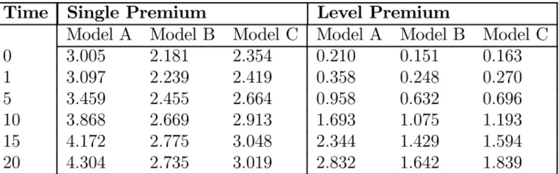
Table 12: Provisions in state 0 for the reversionary annuity.
the deaths of the two are separated by a short spell only, and therefore the shorter the expected period during which annuity installments are payable. Now the premium for Model C is greater than for Model B. Apparently, this is again due to the lower mortality experienced by widows after a year, outweighing the impact of higher mortality in the
first year after getting widowed.
6.2.2 Provisions
Table 12 gives the provisions in state 0 for reversionary annuities. Note again that Model A gives the highest values, and model B the lowest values.
In Table 13, we can view the provisions to be held at several durations when (x) has died and (y) is still alive. Death of the male starts up annuity payments on the life of the surviving female. Needless to say, this is why the provisions in this Table are much higher than the values in Table 12. Since no premiums are due after death, the provisions do not depend on the premium payment arrangement at all.
Like before for the contingent assurance, the provision at duration 20 has been tabu-lated according to various periods elapsed since death of the spouse. Model C now gives thelowest values for death at duration 20. This can be explained by the higher mortality due to short-term dependence, leading to a lower expected present value of future benefits. Further in the table, again just as for the contingent assurance, provisions have been tabulated, where the time of death of the spouse is fixed (at 20), but the contract has been valued at various durations from 20 to 30. For this spell, the provisions go down in time for all three models.
6.2.3 Mortality profit
For an annuity benefit of 1 p.a., the standard deviation of the mortality profit per policy in policy year (t, t+ 1] in Model k, denoted bySDk
t,is calculated as SDkt = q qk y+t ¡ 1−qk y+t ¢ DSARkt,
Time Single Premium, Level premium I/II
Death Valuation Model A Model B Model C
15 20 11.297 8.148 9.145 19 20 11.297 8.148 9.145 19.25 20 11.297 8.148 9.104 19.5 20 11.297 8.148 9.061 19.75 20 11.297 8.148 9.017 20 20 11.297 8.148 8.971 20 20.25 11.459 8.299 9.163 20 20.5 11.624 8.454 9.362 20 20.75 11.792 8.614 9.568 20 21 10.963 7.779 8.781 20 25 9.570 6.312 7.307 20 30 7.741 4.578 5.501
Table 13: Provisions in state 1 or 2 (Model C) or state 1 (Model B) for the reversionary annuity contract.
Duration DSAR EDS S.D. of MP
A B C A B C A B C 0 −17.109 −15.227 −15.870 −0.012 −0.033 −0.050 0.458 0.706 0.888 5 −16.130 −13.881 −14.640 −0.021 −0.056 −0.085 0.588 0.877 1.115 10 −14.949 −12.330 −13.199 −0.037 −0.092 −0.143 0.742 1.059 1.366 15 −13.557 −10.606 −11.563 −0.062 −0.146 −0.232 0.916 1.236 1.620 20 −11.963 −8.779 −9.781 −0.102 −0.223 −0.361 1.099 1.382 1.844 25 −10.209 −6.953 −7.939 −0.161 −0.325 −0.536 1.272 1.468 1.992 30 −8.372 −5.255 −6.155 −0.244 −0.448 −0.750 1.408 1.467 2.014
Table 14: Death Strain at Risk (DSAR), Expected Death Strain (EDS), and Standard Deviation (S.D.) of mortality profit (MP) for a reversionary annuity.
where k indicates the model used,k ∈{A, B, C} and
DSARkt =−t+1Vk−1,
is the death strain at risk in modelk, witht+1Vkbeing the year end provision in Modelk.
Figure 14 gives the results. When compared with the contingent insurance, we see again that the standard deviation of the mortality profit is largest in Model C. Again, this can be ascribed to the high mortality of the widow after death of her partner.
7
Conclusions
The calculations in this paper show that short-term dependence is clearly present. Due to the small number of widows and widowers, however, it is hard to give reliable estimates of the degree of excess mortality. It would have been helpful to have a data set with more contracts and/or a longer period of observation.
With a more extensive data set, it is also possible to allow for different degrees of excess mortality of widow(er)s, for different age ranges. It seems reasonable to assume that the impact of death of the partner is stronger at higher ages, as this usually involves relationships that have lasted longer. In addition, one could argue that lives losing their partner at younger ages have a more extensive social network, and are therefore more able to recover from bereavement.
Acknowledgment
This project is funded by a research grant from the Actuarial Profession in the UK. The authors wish to acknowledge the Society of Actuaries, through the courtesy of Edward (Jed) Frees and Emiliano Valdez, for providing the data used in this paper.
References
[1] Carriere, J.F. (2000). Bivariate survival models for coupled lives. Scandinavian Ac-tuarial Journal., 17-31.
[2] Carriere, J.F. and Chan, L.K. (1986). The bounds of bivariate distributions that limit the value of last-survivor annuities. Transactions of the Society of Actuaries
XXXVIII, 51-74.
[3] Cox, D.R. (1972). Regression models and life tables (with Discussion).Journal of the Royal Statistical Society, Series B, 34, 187-220.
[4] Denuit, M. and Cornet, A. (1999). Multilife premium calculation with dependent future lifetimes. Journal of Actuarial Practice, 7, 147-171.
[5] Denuit, M., Dhaene, J., Le Bailly de Tilleghem, C. and Teghem, S. (2001). Measuring the impact of dependence among insured lifelengths. Belgian Actuarial Bulletin, 1 (1), 18-39.
[6] Frees, E.W., Carriere, J.F. and Valdez, E.A. (1996). Annuity valuation with depen-dent mortality. Journal of Risk and Insurance, 63 (2), 229-261.
[7] Gregorius, F. K. (1993). Disability insurance in the Netherlands. Insurance: Mathe-matics and Economics 13, 101-116.
[8] Haberman, S., and Pitacco, E. Actuarial Models for Disability Insurance, Chapman & Hall/CRC, Boca Raton, 1999.
[9] Hougaard, P. (2000).Analysis of Multivariate Survival Data. Springer.
[10] Jagger, C. and Sutton, C.J. (1991). Death after marital bereavement - is the risk increased? Statistics in Medicine 10, 395-404.
[11] Marshall, A.W. and I. Olkin (1967). A multivariate exponential distribution.Journal of the American Statistical Association, 62, 30-44.
[12] Marshall, A.W. and I. Olkin (1988). Families of multivariate distributions. Journal of the American Statistical Association, 88, 834-841.
[13] Möller, C.M. (1990). Select mortality and other durational effects modelled by par-tially observed Markov chains. Scandinavian Actuarial Journal, 177-199.
[14] Norberg, R. (1988). Select mortality: possible explanations.Transactions of the 23rd international Congress of Actuaries, Helsinki, 3, 215-224.
[15] Norberg, R. (1989). Actuarial analysis of dependent lives. Mitteilungen der Schweiz-erisher Vereinigung der Versicherungsmathematiker, 243-254.
[16] Parkes, C.M., Benjamin, B. and Fitzgerald, R.G. (1969). Broken heart: a statistical study of increased mortality among widowers. British Medical Journal, 740-743. [17] Shemyakin, A. and Youn, H. (2006). Copula models of joint last survivor analysis.
Applied Stochastic Models in Business and Industry, 22, 211-224.
[18] Spreeuw, J. (2006). Types of dependence and time-dependent association between two lifetimes in single parameter copula models. Scandinavian Actuarial Journal,
286-309.
[19] Wolthuis, H. (2003).Life Insurance Mathematics (The Markovian Model). IAE, Uni-versiteit van Amsterdam, Amsterdam, 2nd edition.
[20] Youn, H. and Shemyakin, A. (1999). Statistical aspects of joint life insurance pricing.
1999 Proceedings of the Business and Statistics Section of the American Statistical Association, 34-38.
[21] Youn, H. and Shemyakin, A. (2001). Pricing practices for joint last survivor insurance.