Received 7 June 2003; received in revised form 25 September 2003; accepted 15 December 2003
Abstract
This paper presents a practical method to optimize in-building section of centralized Heating, Ventilation and Air-conditioning (HVAC) systems which consist of indoor air loops and chilled water loops. First, through component characteristic analysis, mathematical models associated with cooling loads and energy consumption for heat exchangers and energy consuming devices are established. By considering variation of cooling load of each end user, adaptive neuro-fuzzy inference system (ANFIS) is employed to model duct and pipe networks and obtain optimal differential pressure (DP) set points based on limited sensor information. A mix-integer nonlinear constraint optimization of system energy is formulated and solved by a modified genetic algorithm. The main feature of our paper is a systematic approach in optimizing the overall system energy consumption rather than that of individual component. A simulation study for a typical centralized HVAC system is provided to compare the proposed optimization method with traditional ones. The results show that the proposed method indeed improves the system performance significantly.
© 2004 Elsevier B.V. All rights reserved.
Keywords: HVAC system; Optimization; Energy conservation; Simulation
1. Introduction
A typical centralized HVAC system is shown as in Fig. 1, which comprises two sections: in-building section and out-building section. It can be further divided into five loops: indoor air loops, chilled water loops, refrigerant loops, condenser water loops and outdoor air loops. The in-building section consists of indoor air loop, chilled water loop and part of refrigerant loop. Indoor air loop includes terminal units, cooling coils, dampers, fans, ducts, and controls. Chilled water loop includes cooling coils, chiller evaporators, pumps, pipes, valves, and controls[1]. In terms of energy consumption, the components of in-building sec-tion account for large porsec-tion of total energy used in HVAC systems. A small increase in operating efficiency can result in substantial energy savings. In practice, however, optimal operation for such a system is not an easy task as there are thousands of rooms and hundreds of cooling coils in a large-scale HVAC system and all these components are closely coupled.
Targeted at energy conservation, there have been many research works reported either for individual component ef-ficiencies or part of system efef-ficiencies. For the cooling
∗Corresponding author. Tel.:+65-67906862; fax:+65-67905471.
E-mail address: [email protected] (W. Cai).
coil model, Stoecker[2]provided a model with many em-pirical parameters under the assumptions of constant air-flow and water air-flow. Unfortunately, these assumptions are no longer valid in modern HVAC systems. Braun [3] and Rabehl[4] gave their cooling coil models through detailed analysis, unfortunately, both models are somewhat compli-cated and iterative computations are required. The energy saving potential using variable speed drive (VSD) pumps in chilled water loop is an attractive subject which has at-tracted many researchers’ interests [5–7]. Note that these works only considered the individual element without link-ing it to the whole system energy consumption. The effi-ciencies of pumps and fans were also studied in[8,9], where efficiencies of pumps and fans and required pump heads are assumed to be constants which are approximations for con-stant speed fans and pumps and fixed DP controls, respec-tively. If VSD pumps/fans and variable pump/fan pressure set points are used, the total pump/fan efficiencies may vary from 80 to 40%.
For the duct and pipe networks, some researchers only considered simple systems and some considered all the cool-ing coils with the same coolcool-ing loads simultaneously, which is not true in practice. House and Smith[10]studied opti-mization of two-zone variable air volume (VAV) heating sys-tem by traditional derivative-based methods, which would become very complicated if the number of zones is more than two. Assuming all the cooling loads of coils were 0378-7788/$ – see front matter © 2004 Elsevier B.V. All rights reserved.
Nomenclature
a0, a1, a2 the constant coefficients to determine PLRadj,i
b0,. . ., b5 the constant coefficients to determine Tempadj,i,
c1, c2, c3 the constant coefficients in cooling coil models
COPnom the nominal coefficient of performance of chillers
COPnom,i the nominal coefficient of performance of the ith chiller
DL the diversity level
gc the constant
f1,. . ., f5 the functions
hk,l the enthalpy of the ith room air cooled by kth cooling coil
hSA,k the enthalpy of supply air provided by the kth cooling coil
HCHW the pump head provided by chilled water pumps
HCHW,j the pump head provided by the jth chilled water pump
HSA the air pressure provided by cooling coil fans
HSA,k the air pressure provided by the kth cooling coil fan
i the number of chillers
j the number of chilled water pumps
k the number of cooling coil fans
l the number of rooms
ma the airflow rate
mCHW the chilled water flow rate through cooling coils
mCHW,j the chilled water flow rate through thejth chilled water pump
mCHW,k the chilled water flow rate to the kth cooling coil
mCW the condenser water flow rate through chillers
mSA the airflow rate of supply air through cooling coils
mSA,k the airflow rate of supply air through the kth cooling coil
mSA,k,l the airflow rate of supply air through the
kth cooling coil to the ith room mw the water flow rate
M1 the maximum number of fuzzy rules
M2 the maximum number of input of ANFIS
N1 the number of operating chillers
N2 the number of operating chilled water pumps
N3 the number of operating cooling coil fans
N4 the number of conditioned rooms
oi,k the adaptive coefficients in ANFIS
Pchiller the power consumption of chillers
Pfan the power consumption of fans
Ppump the power consumption of pumps
Ptotal the total power consumption of the whole system
Pbcrossover the probability of crossover rate Pbmutation the probability of mutation rate PLRadj the part-load ratio adjustment factor
of chillers
PLRadj,i the part-load ratio adjustment factor of the ith chiller
Q the cooling capacity provided by chillers
Qcap the nominal cooling capacity of chillers
Qcap,i the nominal cooling capacity of the
ith chiller
Qcoil the heat exchange rate of cooling coils
Qi the real cooling capacity provided by the ith chiller
Qk,l the cooling load of the lth room provided by the kth cooling coil
TCHWS the temperature of the chilled water supply
TCWS the temperature of condenser water supply
TCWR the temperature of condenser water return
TMA the temperature of mixed air entering cooling coils
TMA,k the temperature of mixed air entering the
kth cooling coil
Twb the wet-bulb temperature of air leaving coil Tempadj the temperature adjustment factor of
chillers
Tempadj,i the temperature adjustment factor of the
ith chiller
xi2 the i2th input of ANFIS
y the output of ANFIS
ηCHW the total efficiency of the chilled water pumps
ηCHW,j the total efficiency of the ith chilled water pump
ηSA the total efficiency of the cooling coil fans ηSA,k the total efficiency of the kth cooling
coil fan
µ(c) the fuzzy number of linguistic variable c
same, Wepfer and Shelton [11]described the optimization of chilled water rate as a function of the air-water coil size and the refrigerant-water coil size. Braun[8] and Ahn [12]described indoor air loops and chilled water loops with quadratic functions, which is not accurate when the cooling loads of end users are changing diversely.
For the whole system optimization, Austin [13] and Kirsner[14]used real systems for experiments and summa-rized some general ideas, which is difficult to be extended to other systems for precisely optimal control. Hartman [15] pointed out that an integrated DDC provides new
Fig. 1. Schematic of a typical HVAC system. approaches to improve energy efficiencies and comfort of
typical facilities significantly. But very large amount of data places huge burdens on communication network and processing capacities of DDC systems.
As for optimization algorithms, the classic derivative-based methods are widely used [3,10–12], but they are inca-pable of dealing with mixed-integer nonlinear optimization. Thanks to the newly developed evolutionary computation techniques, genetic algorithms have been successfully used in many areas[16–19]. In order to relieve huge burdens on DDC systems, original optimization problem is simplified to reduce number of independent variables and computation time.
For validation of computational models of HVAC com-ponents, Salsbury and Diamond [20]had successfully val-idated model-based energy analysis of HVAC systems by comparing a real system with simulations. Although the real system is of a relatively small scale—dual-duct air handling unit (AHU), it provides an approach to simulate real systems based on component models.
In this paper, we present a systematic approach opti-mal set point control for in-building section. Major com-ponents of in-building section are analyzed to identify the energy conservation potential. For the sake of real time system optimization, simple but accurate component mod-els are selected to flexibly fit all kinds of modem systems, such as VAV systems, variable chilled water systems, and variable temperature controlled chiller systems. In order to save energy for delivery of supply air and chilled water, a variable pressure set point method is analyzed by a simple example and an intelligent neural network model-ANFIS is proposed to compute the variable pressure set points influ-enced by variation of cooling loads of end users. Based on these models, a mix-integer nonlinear constraint optimiza-tion problem is then formulated. A modified genetic algo-rithm is devised for this particular problem to find optimal set points to minimize the overall system energy consump-tion. Consequently, the optimal set points are implemented to show the advantages of the proposed method through simulations.
The rest of the paper is organized as follows. Section 2 presents the modeling of cooling coils, chillers, pumps and
fans. The analysis of duct and pipe networks is given in Section 3. The optimization of system energy consumption is described thoroughly inSection 4. Simulations and com-parisons are carried out inSection 5. Finally, some conclu-sions are drawn inSection 6.
2. Characteristics of components
The heat exchangers and energy consuming devices of in-building section are cooling coils, chillers, pumps and fans.
2.1. Cooling coil
The heat transfer rate of a cooling coil is influenced by the following parameters: the temperature of air entering coil (TMA), the chilled water supply temperature (TCHWS), and the mass flow rates of supply air and chilled water (mSA and mCHW).Fig. 2describes the relationship of a common crossflow cooling coil with six-row derived from manufac-ture data.
Without loss of generality, the enthalpy of air and temper-ature of chilled water entering coil are assumed to be con-stants and the relative humidity of air leaving coil is assumed as 90%. The wet-bulb temperature of air leaving coil is de-noted as Twbin the figure. The performance of the cooling coil follows:
• For a given heat transfer rate (Qcoli) different air tempera-ture set points require different air to water flow rate ratio. For example, at Twb = 12◦C and 60% of nominal heat transfer rate, the ratio is 0.82, whereas atTwb=15◦C the ratio is 2.63.
• For a varying coil heat transfer rate, same temperature set point also results in different air to water flow rate ratio. For example, atTwb=13◦C, 60% of nominal heat transfer rate requires the air to water flow rate ratio of 1.21, whereas, 90% of nominal heat transfer rate requires the air to water flow rate ratio of 0.94.
In order to relate heat transfer rates of cooling coils to other input variables directly, the following model [21]is adopted to show the performance of cooling coil.
Qcoli= c1mcSA3
1+c2(mCHW/mSA)c3(TMA−TCHWS) (1)
Compared with other models[2–4], this model does not need iterative computations, which makes it suitable for real time implementation. In this model, no geometric data of coils are required and only three empirical parameters (c1, c2and
c3) need to be identified from manufacture catalog data or experiment data.
2.2. Chiller
The performance of chiller is influenced by several fac-tors: chilled water supply temperature (TCHWS), condenser water supply temperature (TCWS), cooling load (Q). Since this paper focuses on in-building section, the condenser wa-ter supply temperature is considered as a constant.Fig. 3 [22] illustrates the coefficient of performance (COP) of a commonly used centritugal chiller with respect to chilled water supply temperatures and cooling loads.
As is shown inFig. 3, higher TCHWSset points make the chiller consume less energy. Whereas, the chiller uses more energy at lower TCHWSset points. Although lower TCHWSset points waste chiller energy, it saves energy of chilled water pumps. The optimal temperature set points exist when the summation power consumption of both chillers and pumps is minimal.
For multi-chiller system, the ideal method of sequencing chillers is to make all the operating chillers running around the most efficient points.
To clearly express the relationship between power con-sumption of chillers and other related parameters, Stoecker’s model[2]below is adopted.
Pchiller=Qcap·COPnom·(PLRadj)·(Tempadj) (2a)
Fig. 3. The performance of a centrifugal chiller. where PLRadj=a0+a1 Q Qcap +a2 Q Qcap 2 (2b) Tempadj=b0+b1TCHWS+b2TCHWS2 +b3TCWS +b4T2 CWS+b5TCHWSTCWS (2c) The parameters, a0–a2 and b0–b5, are acquired from the manufacture catalog data or experiments by common curve-fitting methods.
2.3. Pumps and fans
The power consumptions of VSD driven pumps and fans are influenced by two parameters: mass flow rates of fluids and the pressure difference between the inlets and outlets. Since the characteristics of pumps and fans are very similar, we only use pump performance to demonstrate their prop-erties.
Fig. 4shows a pump performance curve. The total effi-ciency including motor effieffi-ciency, pump effieffi-ciency, and VSD efficiency, is water flow rate and total pump head, but in a more complex format.
The general model[1]to describe pump and fan energy consumption is shown in Eq. (3).
Ppump= mCHWHCHW
gcηCHW
orPfan= mSAHSA
gcηSA for fans
(3a) where,
ηCHW =f1(mCHW, HCHW)
(orηSA=f2(mSA, HSA)for fans) (3b) The functions to express the total efficiencies of pumps and fans, f1and f2, can be polynomials, neural networks, or any other curve-fitting representations.
Fig. 4. A pump performance curve.
3. Analysis of duct and pipe networks
The duct and pipe networks are the important components of in-building section of HVAC systems. Since the structures of duct and pipe networks are only slightly different, the
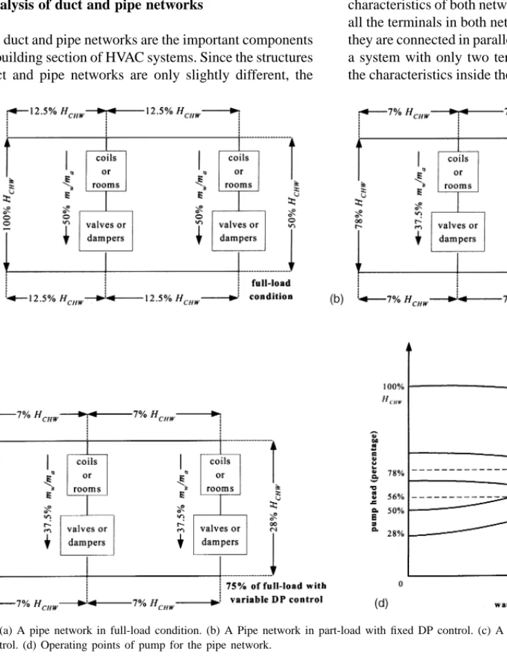
Fig. 5. (a) A pipe network in full-load condition. (b) A Pipe network in part-load with fixed DP control. (c) A pipe network in part-load with variable DP control. (d) Operating points of pump for the pipe network.
characteristics of both networks are very similar. In addition, all the terminals in both networks have the same feature and they are connected in parallel, generally. It is sufficient to use a system with only two terminals (Fig. 5a) to demonstrate the characteristics inside the system. For simplicity, only the
analysis of the pipe networks is discussed and the concept can be extended to systems with more terminals and also duct networks.
3.1. A simple system with two terminals
The theoretical analysis of a system with two terminals at full-load condition is shown inFig. 5a. The structures and designed mass flow rates of both terminals are identical. The total required pump head is denoted as HCHWand the head loss in pipe network is expressed referring to percentage of
HCHW. The required DP of the furthest terminal at full-load condition is 50% of HCHW.
The conventional control strategy to operate the system under part-load condition is to keep the furthest terminal at a fixed DP set point. The detailed information at 75% of full-load with symmetric load distribution is shown in Fig. 5b. The total required pump head is 78% of HCHW and the DP set point is 50% of HCHW.
In comparison with the conventional method, the variable DP set point control strategy is used in the same system with the same cooling load distribution. The concept of this strategy is to keep at least one control valve in fully-open condition. The detail information is shown inFig. 5c. The total required pump head is 56% of HCHW and the DP set point is 28% of HCHW.
If a dedicated pump is employed to deliver water to the system, the pump operating points for three conditions are visualized inFig. 5d. The designed operating point at full-load condition is at point A. Since the cooling load dis-tribution of 75% full-load is symmetric, the system curve is same with the full-load condition. The operating point of conventional method is at point B1, while the variable DP control is operating at point B2. According to Fig. 4, the pump power is a monotonous function with respect to pump head when flow rate is a fixed value. Undoubt-edly, the pump uses less energy at point B2 than at point B1.
Fig. 6. The Architecture of ANFIS.
The disadvantage of the latter control strategy is that DP set points are too difficult to determine for asymmetric cooling load with hundreds of terminals. The major prob-lem is to determine pressure loss in each part of duct and pipe networks. In practical, we do not have enough sensors to provide sufficient information for function loss of each part. If the design data of duct and pipe networks are used directly, any little error will cause significant discrepancy between calculated and real control actions. This prevents the control method from being implemented. Fortunately, an intelligent neural network, ANFIS, can be employed to solve the problem and it is proved a workable approach [23].
3.2. ANFIS models for duct and pipe networks
ANFIS is a fuzzy inference system implemented in the framework of adaptive neural networks[24]. Because there are almost no limitation on its network structures and node functions, it has been successfully employed in a wide va-riety of applications of modeling, decision making, signal processing and control. The architecture of ANFIS for solv-ing the variable DP set points of indoor air loops and chilled water loops is shown inFig. 6, which is a multi-layer feed-forward network.
The functions of each layer are summarized as follows [23]:
• Layer 1: The crispy variables are divided into several lin-guistic variables.
• Layer 2: This layer outputs the fuzzy number of each linguistic variable.
• Layer 3: A rule base of the fuzzy inference system is embodied in this layer.
• Layer 4: The weight of each fuzzy rule is evaluated in this layer.
• Layer 5: All the outputs of Layer 4 are aggregated to calculate the output.
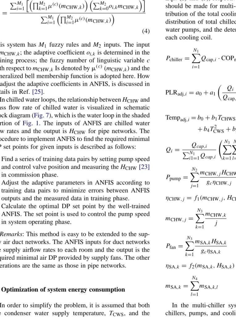
Fig. 7. Schematic block diagram of a chilled water loop. The whole ANFIS can be written into an equation format as the following: f3(mCHW,k) = M1 i=1 M2 k=1µ(c)(mCHW,k) M 2 k=0oi,kmCHW,k M1 i=1 M2 i=1µ(c)(mCHW,k) (4) This system has M1 fuzzy rules and M2 inputs. The input is mCHW,k; the adaptive coefficient oi,kis determined in the training process; the fuzzy number of linguistic variable c with respect to mCHW,kIs denoted by(c)(mCHW,k) and the generalized bell membership function is adopted here. How to adjust the adaptive coefficients in ANFIS, is discussed in details in Ref.[25].
In chilled water loops, the relationship between HCHWand mass flow rate of chilled water is visualized in schematic block diagram (Fig. 7), which is the water loop in the shaded portion ofFig. 1. The inputs of ANFIS are chilled water flow rates and the output is HCHW for pipe networks. The procedure to implement ANFIS to find the required minimal DP set points for given inputs is described as follows: 1. Find a series of training data pairs by setting pump speed
and control valve position and measuring the HCHW[23] in commission phase.
2. Adjust the adaptive parameters in ANFIS according to training data pairs to minimize errors between ANFIS outputs and the measured data in training phase. 3. Calculate the optimal DP set point by the well-trained
ANFIS. The set point is used to control the pump speed in system operating phase.
Remarks: This method is easy to be extended to the
sup-ply air duct networks. The ANFIS inputs for duct networks are supply airflow rates to each room and the output is the required minimal air DP provided by supply fans. The other operations are the same as those in pipe networks.
4. Optimization of system energy consumption
In order to simplify the problem, it is assumed that both the condenser water supply temperature, TCWS, and the
minimize total power consumption of the in-building section and is given in Eq. (5).
Objective function : minPtotal=Pchiller+Ppump+Pfan (5a) In Eq. (5), the expressions for power consumption of chillers
Pchiller, pumps Ppump and fans Pfan follow the format in Eqs. (2) and (3), respectively. However, some adjustments should be made for multi-chiller Systems, such as the dis-tribution of the total cooling load to each operating chiller, distribution of total chilled water flow rate to each chilled water pumps, and the determination of airflow rate through each cooling coil.
Pchiller = N1
i=1
Qcap,i·COPnom,i·(PLRadj,i)·(Tempadj,i) (5b) PLRadj,i=a0+a1 Qi Qcap,i +a2 Qi Qcap,i 2 (5c) Tempadj,i=b0+b1TCHWS+b2TCHWS2 +b3TCWS +b4T2 CWS+b5TCHWSTCWS (5d) Qi= NQ1cap,i i1=1Qcap,i N 3 k=1 N4 l=1 Qk,l (5e) Ppump= N2 j=1 mCHW,jHCHW gcηCHW,j (5f) ηCHW,j=f1(mCHW,j, HCHW) (5g) mCHW,j= N3 k=1 mCHW,k j (5h) Pfan = N3 k=1 mSA,kHSA,k gcηSA,k (5i)
ηSA,k =f2(mSA,k, HSA,k) (5j)
mSA,k = N4
l=1
mSA,k,l (5k)
In the multi-chiller system, the numbers of operating chillers, pumps, and cooling coils are denoted as N1, N2,
and N3, respectively. Each cooling coil provides cooling load for N4rooms. Without loss of generality, all the chillers are assumed to be of the same type and have the similar characteristics. Both pumps and fans are assumed to be the centrifugal ones.
The objective function of Eq. (5) subjects to the following constraints:
Constraint (1). All the following variables should be within
their own upper and lower bounds. TCHWS, mCHW,j, HCHW,
mCHW,k, mSA,k,l, HSA,k,hSA,k ∈[min, max].
Constraint (2). The chilled water pumps should
con-vey enough water to all the cooling coils. HCHW,j =
f3(mCHW,k)(k=1, . . . , N3).
Constraint (3). Each cooling coil should bring enough
cooling capacity to supply airflow. Refer to Eq. (1);
Constraint (4). The cooling coil fans should deliver
enough airflow to all terminals.HSA,k =f4(mSA,k,l)(k = 1, . . . , N3;l=1, . . . , N4);
Constraint (5). The supply air to rooms should provide
enough cooling load for all the rooms.Qk,l=mSA,k,l(hk,l−
hSA,k)(k=1, . . . , N3; l=1, . . . , N4);
Notes: The function f3and f4 are represented byEq. (4) for the variable DP set points control strategy.
The above described optimization problem has many variables—continuous and discrete ones. It also has many non-linear constraints to be satisfied. Furthermore, the AN-FIS structure of Constraints (2) and (4) is difficult to acquire their derivatives. These three obstacles make the optimiza-tion impossible using classical optimizaoptimiza-tion methods. The emerging computation method-genetic algorithms, there-fore, is adopted and will be introduced in detail in the later section. In order to use genetic algorithms in an efficient way, simplification process is introduced with consideration of the system interior features.
For a large scale HVAC system, the energy consumption of the whole system, Ptotal, could be a function of hun-dreds of variables: Qk,l, TCWS, TMA,k, i, j, k, TCHWS, mSA,k,l,
mCHW,k, HCHW,j, HSA,k, as shown in the Eq. (5). It is ineffi-cient and impractical to optimize all of them as a whole. All the variables affecting the objective can be divided into three groups: uncontrollable variables, independent variables and dependent variables.
Uncontrollable variables include Qk,l, TCWS, and TMA,k. Because the cooling load of each rooms and the mixed air dry bulb temperature are determined by heat gain from outside environment and inside activities. Both factors can not be controlled by the control system. Another variable condenser water supply temperature is controlled by condenser water loops and is considered as uncontrollable to the indoor air loops and chilled water loops.
Independent variables include i, j, k, TCHWS, and mSA,k,l. Among them, i, j, and k are discrete control variables; TCHWS and mSA,k,lare continuous control variables. With these vari-ables, the rest of control variables can be determined by constraints.
Dependent variables include mCHW,k, HCHW,j, HSA,k. Once Qk,l (k = 1, . . . N3;l = 1, . . . , N4), TMA,k (k = 1, . . . N3), TCHWS, and mSA,k,l (k = 1, . . . N3; l = 1, . . . , N4) are known, mCHW,k (k = 1, . . . N3) are de-termined uniquely by characteristics of cooling coils in Constraint (3). Furthermore, mSA,k,lis also limited by Con-straint (1), and the range of hk,l. If the ANFIS structure and parameters in Constraint (2), f3, is determined, HSA,k (k = 1, . . . N3) are only dependent on mSA,k,l. Similarly,
HCHW,j (j = 1, . . . , N2) can also be treated as dependent variables of mass flow rates, mCHW,k (k = 1, . . . N3), by applying Constraint (4).
For the uncontrollable variables, they can be measured during one sample period and treated as constants for the optimization problem. Independent variables can be treated as the input variables of optimization problem. Dependent variables are determined by independent variables uniquely with the help of constraint conditions. Consequently, the objective function can be rewritten in the following format with Constraints (1) and (5).
Ptotal=f5(i, j, k, TCHWS, mSA,k,l) (6)
With a set of input variables (i, j, k, TCHWS, and mSA,k,l) and fixed uncontrollable variables (Qk,l, TCWSand TMA,k), Eq. (6)has a unique total power consumption value of the whole system. Through the optimization algorithm, a set of optimal input variables, which has the minimal system power consumption, can be found.
4.2. Optimization algorithms
Considering the complexity of this optimization problem, a modified genetic algorithm is adopted to solve the partic-ular case.
4.2.1. Representation: genetic encoding
An important aspect of genetic algorithm is coding or representation. It is the process of transforming a problem into a serial of codes that can be easily interpreted, and can be used in evaluation of the information it represents using the fitness function. In this case, the independent variables, (i, j, k; TCHWS, mSA,k,l), are changed into binary strings and are connected together to form a chromosome. The lower and upper bounds of the binary variables are the minimum and maximum values of set points limited by Constraint (1). The lengths of binary strings are determined by the control precision of corresponding variables. It means that a more precise set point control requires a longer binary string.
Ptotal+penalty
Since the optimization objective is to find minimal value of
Ptotal, the penalty value should be a positive number when the constraints are not fulfilled. The penalty function also should be large enough to avoid the corresponding chromo-some being selected as the optimal value. It would be better if it can provide information for the next step to direct the so-lutions to the feasible region. Before the fitness value being used for evolution operation, a simple linear scaling function is used to adjust the fitness values of each chromosome.
4.2.3. Evolution operation
In reproduction process, elitist roulette wheel selec-tion is proved [26] relatively efficient and adopted here. Single-point crossover and single-bit mutation operators [27]are adopted to produce the next generation. In order to maintain the diversity of population and avoid the prema-ture problem, a definition of diversity level (DL) is given inEq. (8) and it will be used to change the probability of crossover rate and mutation rate.
DL= best population fitness value
average population fitness value (8) The value of DL ranges from unit to positive infinity. When DL equal to unit, it means all the chromosomes in population have the same fitness value and the diversity level is the lowest. The probabilities of crossover rate and mutation rate are expressed in the following equations.
Pbcrossover = 1 1+e(1−DL) (9) Pbmutation = e(1−DL) 1+e(1−DL) (10)
The probability of crossover rate will tend to 0.5 when the evolution tends to premature, while the probability of mu-tation rate will increase significantly to diversify the popu-lations. When the diversity level of population is high, the probability of mutation rate is restricted nearly to zero and crossover operation will dominate.
4.2.4. Termination
The computation of genetic algorithms is terminated when the following criteria are reached.
• The maximum number of generations is reached;
• The fitness value of the best chromosome converges to some asymptote.
mSA,k,l) in searching space;
For generation=1: max generation;
Compute the fitness of each individual in the old population;
Store the highest fitness of individual;
Evaluate the diversity level and determine probability rates;
Use “elitist roulette wheel” selection method to form mating pool;
While individual number<population size do; Select two parents from the mating pool randomly; Perform crossover and mutation operation to
pro-duce offsprings;
Place the offspring to new population; Enawhile
Replace the old population by the new population; Replace the least fitness of individual in new population
by stored highest one; Endfor
Output the individual of the highest fitness based on input variables in real time.
To show the performance of the modified genetic algo-rithm,Fig. 8is the convergence curves of individuals with the minimal objective function values in each generation. The optimization starts with three randomly selected initial populations for the same problem. The population size of each generation is 50. In the end of evolution-the 100th gen-eration, the best individuals in the three populations are all convergent to the same optimal point.
After optimization, a set of optimal independent vari-ables (i, j, k; TCHWS, mSA,k,l is found corresponding to a certain condition (Qk,l, TCWS, TMA,k). However, it cannot be implemented directly due to some practical limitations. Considering the control strategies in real HVAC sys-tems, the implementation issues are introduced in the next section.
4.3. Implementation Issues
The first step to implement the model-based optimization is to find the component model parameters which are con-stants inEqs. (1)–(4). These models can be determined by manufacture catalog data or on-site testing data.
The second step is to collect the uncontrollable variables (Qk,l, TCWS, TMA,k) by real time measurement. The variables are considered constants during one sampling period.
The third step is to start the optimization procedure as described in the previous section and find the optimal inde-pendent variables (i, j, k; TCHWS, mSA,k,l).
Fig. 8. Convergence curves of the modified genetic algorithm.
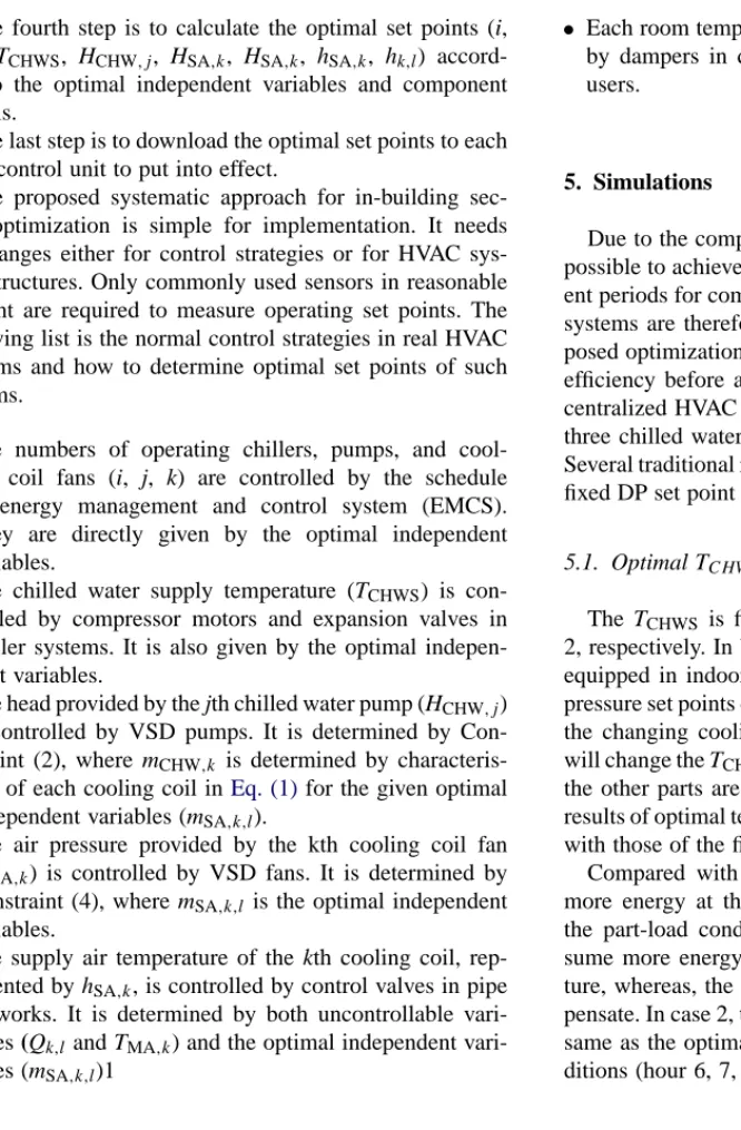
The fourth step is to calculate the optimal set points (i,
j, k, TCHWS, HCHW,j, HSA,k, HSA,k, hSA,k, hk,l) accord-ing to the optimal independent variables and component models.
The last step is to download the optimal set points to each local control unit to put into effect.
The proposed systematic approach for in-building sec-tion optimizasec-tion is simple for implementasec-tion. It needs no changes either for control strategies or for HVAC sys-tem structures. Only commonly used sensors in reasonable amount are required to measure operating set points. The following list is the normal control strategies in real HVAC Systems and how to determine optimal set points of such systems.
• The numbers of operating chillers, pumps, and cool-ing coil fans (i, j, k) are controlled by the schedule of energy management and control system (EMCS). They are directly given by the optimal independent variables.
• The chilled water supply temperature (TCHWS) is con-trolled by compressor motors and expansion valves in chiller systems. It is also given by the optimal indepen-dent variables.
• The head provided by the jth chilled water pump (HCHW,j) is controlled by VSD pumps. It is determined by Con-straint (2), where mCHW,k is determined by characteris-tics of each cooling coil inEq. (1)for the given optimal independent variables (mSA,k,l).
• The air pressure provided by the kth cooling coil fan (HSA,k) is controlled by VSD fans. It is determined by Constraint (4), where mSA,k,l is the optimal independent variables.
• The supply air temperature of the kth cooling coil, rep-resented by hSA,k, is controlled by control valves in pipe networks. It is determined by both uncontrollable vari-ables (Qk,land TMA,k) and the optimal independent vari-ables (mSA,k,l)1
• Each room temperature, represented by hk,l, is controlled by dampers in duct network. It is determined by room users.
5. Simulations
Due to the complexity of HVAC system, it is almost im-possible to achieve same cooling load profiles at two differ-ent periods for comparison. Some simulations based on real systems are therefore used to show advantages of the pro-posed optimization method. In order to compare the energy efficiency before and after optimization, a simulation of a centralized HVAC system with 60 rooms, 15 cooling coils, three chilled water pumps, and three chillers is conducted. Several traditional methods, such as fixed TCHWScontrol and fixed DP set point control, are studied here for comparison.
5.1. Optimal TCHWSversus fixed TCHWS
The TCHWS is fixed at 7◦C in case 1 and 9◦C in case 2, respectively. In both cases, the VSD fans and pumps are equipped in indoor air loops and chilled water loops. The pressure set points controlled fans and pumps are varied with the changing cooling load. The proposed optimal method will change the TCHWSwith the changing cooling load, while the other parts are the same as the case 1 and case 2. The results of optimal temperature set point control are compared with those of the fixed TCHWScontrol inFig. 9.
Compared with optimal method, case 1 consumes 7% more energy at the full-load condition and about 10% at the part-load condition. This is because the chillers con-sume more energy to lower chilled water supply tempera-ture, whereas, the saved pump energy is too small to com-pensate. In case 2, the total power consumption is almost the same as the optimal results except for some part-load con-ditions (hour 6, 7, 20, 21, and 22). The reason is that most
Fig. 9. Comparison between variable and fixed TCHWS.
of the calculated optimal set points of chilled water supply temperature are 9◦C.
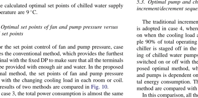
5.2. Optimal set points of fan and pump pressure versus fixed set points
For the set point control of fan and pump pressure, case 3 uses the conventional method, which provides the furthest terminal with the fixed DP to make sure that all the terminals can be provided with enough air and water. In the proposed optimal method, the set points of fan and pump pressure vary with the changing cooling load in each room or coil. The results of two methods are compared inFig. 10.
In case 3, the total power consumption is almost the same as that in the optimal method at full-load condition. The energy saving of optimal method lies in part-load conditions and it ranges from 40% at low part-load to 10% at high part-load.
Fig. 10. Comparison between variable and fixed pressure set point control.
Fig. 11. Comparison of optimal and tradition sequencing.
5.3. Optimal pump and chiller sequencing versus increment/decrement sequencing
The traditional increment/decrement sequencing method is adopted in case 4, where the additional chiller is staged on when the cooling load above a certain value, for exam-ple 90% of total operating chiller capacities, and the extra chiller is staged off in the same manner. For the sequenc-ing of chilled water pumps in traditional method, they are switched on or off with the dedicated chillers. For the pro-posed optimal method, when to switch on or off chillers and pumps is dependent on the objective of minimizing to-tal energy consumption. The results of optimal sequencing method are compared with traditional one inFig. 11.
In this comparison, all the control strategies and set points of controllable variables are same except for sequencing method. Obviously, the optimal sequencing method saves energy usage compared with the traditional method at the part-load condition. While at the high part-load and full-load condition, the total power consumption are same for both sequencing methods. This is because that both sequencing methods make the same decision during that period—using all the pumps and chillers.
5.4. Comparison of energy usage of different cases for 24 hours
The 24 h summations of system energy usage are com-pared inFig. 12between optimal method and different cases. It is no doubt that the optimal method consumes the least energy among all the cases. Summarize the optimal method as follows:
• Finding the optimal set points of chilled water supply temperature with the variation of total cooling load.
• Changing the optimal set points of cooling coil fan pres-sure and chilled water pump prespres-sure with the variation of cooling load in each room and each coil.
Fig. 12. The 24 h summations of system energy usage.
• Sequencing the operating pumps and chillers according to optimal decision with the variation of total cooling load.
6. Conclusions
Through analysis of the characteristics of components and interaction between components, a model-based optimiza-tion problem for in-building secoptimiza-tion is formulated. A mod-ified genetic algorithm is adopted to solve the problem and find the optimal set points of the controllable variables. From the simulation results, the system energy usage can be min-imized by operating components at the optimal set points calculated in real time with the changing cooling load. The optimal set points include chilled water supply temperature, chilled water pump head, air differential pressure in duct networks, and sequencing of pumps and chillers.
References
[1] ASHRAE, ASHRAE Handbook-Fundamentals, American Society of Heating, Refrigerating and Air-Conditioning Engineers Inc., 1997. [2] W.F. Stoecker, Procedures for Simulating the Performance of
Com-ponents and Systems for Energy Calculations, ASHRAE, New York, 1975.
[3] J.E. Braun, Methodologies for design and control of central cooling plants, Ph.D. Thesis, Department of Mechanical Engineering, Uni-versity of Wisconsin, Madison, 1988.
[4] R.J. Rabehl, J.W. Mitchell, W.A. Beckman, Parameter estimation and the use of catalog data in modeling heat exchangers and coils, HVAC&R Research 5 (1) (1999) 3–17.
[5] O. Ahmed, DDC applications in variable-water-volume systems, ASHRAE Transactions 97 (1) (1991) 751–758.
[6] L. Tillack, J.B. Rishel, Proper control of HVAC variable speed pumps, ASHRAE Journal 40 (11) (1998) 41–47.
[7] H. Bynum, E. Merwin, Variable flow—a control engineer’s perspec-tive, ASHRAE Journal 41 (1) (1999) 26–30.
[8] J.E. Braun, S.A. Klein, J.W. Mitchell, W.A. Beckman, Application of optimal control to chilled water system without storage, ASHRAE Transactions 95 (1) (1989) 663–675.
[9] M.A. Cascia, Implementation of a near-optimal global set point control method in a DDC controller, ASHRAE Transactions 106 (1) (2000) 249–263.
[10] J.M. House, T.F. Smith, A system approach to optimal control for HVAC and building systems, ASHRAE Transactions 101 (2) (1995) 647–660.
[11] W.J. Wepfer, S.V. Shelton, Chilled-water loop optimization, ASHRAE Transactions 96 (2) (1990) 656–661.
[12] B.C. Ahn, J.W. Mitchell, Optimal control development for chilled water plants using a quadratic representation, Energy and Buildings 33 (4) (2001) 371–378.
[13] S.B. Austin, Chilled water system optimization, ASHRAE Journal 35 (7) (1993) 50–56.
[14] W. Kirsner, Designing for 42◦F chilled water supply temperature— does it save energy? ASHRAE Journal 40 (1) (1998) 37–42. [15] T.B. Hartman, Global optimization strategies for high-performance
controls, ASHRAE Transactions 101 (2) (1995) 679–687. [16] Y. Asiedu, R.W. Besant, P. Gu, HVAC duct system design
us-ing genetic algorithms, HVAC&R Research 6 (2) (2000) 149– 173.
[17] T.T. Chow, Q.G. Zhang, Z. Lin, C.L. Song, Global optimization of absorption chiller system by genetic algorithm and neural network, Energy and Buildings 34 (2002) 103–109.
[18] A.S. Dragan, A.W. Godfrey, Genetic operators and constraint han-dling for pipe network optimization, Lecture Notes in Computer Science, AISB Workshop Sheffield, Springer, 1995.
[19] W. Huang, H.N. Lam, Using genetic algorithms to optimize controller parameters for HVAC systems, Energy and Buildings 26 (1997) 277– 282.
[20] T. Salsbury, R. Diamond, Performance validation and energy analysis of HVAC systems using simulation, Energy and buildings 32 (1) (2000) 5–17.
[21] Y. Wang, W. Cai, Y.C. Soh, S. Li, L. Xie, An engineering model of coils and heat exchangers for HVAC system simulation and opti-mization, in: 2nd WSEAS International Conference on Simulation, Modeling and Optimization, Greece, 2002.
[22] J.F. Kreider, A. Rabl, Heating and Cooling of Buildings—Design and Efficiency, McGraw-Hill, 1994.
[23] L. Lu, W. Cai, S. Li, L. Xie, Y.C. Soh, Application of ANFIS in chilled water distribution processes for energy savings, The 2002 International Conference on Control and Automation, Xiamen, China, 2002.
[24] J.S. Jang, C.T. Sun, E. Mizutani, Neuro-Fuzzy and Soft Computing: A Computation Approach to Learning and Machine Intelligence, Prentice-Hall International, 1997.
[25] J.S. Jang, Adaptive-network-based fuzzy inference system, IEEE Transactions on Systems, Man, and Cybernetics 23 (3) (1993) 665– 685.
[26] M. Sakawa, K. Kato, H. Sunada, T. Shibano, Fuzzy programming for multiobjective 0-1 programming problems through revised genetic algorithms, European Journal of Operational Research 97 (1997) 149–158.
[27] D.E. Goldberg, Genetic Algorithms in Search-Optimization and Ma-chine Learning, Addison-Wesley, Massachusetts, 1989.