econstor zbw

econstor

www.econstor.eu

Der Open-Access-Publikationsserver der ZBW – Leibniz-Informationszentrum Wirtschaft

The Open Access Publication Server of the ZBW – Leibniz Information Centre for Economics

Nutzungsbedingungen:

Die ZBW räumt Ihnen als Nutzerin/Nutzer das unentgeltliche, räumlich unbeschränkte und zeitlich auf die Dauer des Schutzrechts beschränkte einfache Recht ein, das ausgewählte Werk im Rahmen der unter

→ http://www.econstor.eu/dspace/Nutzungsbedingungen nachzulesenden vollständigen Nutzungsbedingungen zu vervielfältigen, mit denen die Nutzerin/der Nutzer sich durch die erste Nutzung einverstanden erklärt.

Terms of use:

The ZBW grants you, the user, the non-exclusive right to use the selected work free of charge, territorially unrestricted and within the time limit of the term of the property rights according to the terms specified at

→ http://www.econstor.eu/dspace/Nutzungsbedingungen By the first use of the selected work the user agrees and declares to comply with these terms of use.

zbw

Han, Heejoon; Kutan, Ali M.; Ryu, Doojin

Working Paper

Modeling and predicting the market volatility index:

The case of VKOSPI

Economics Discussion Papers, No. 2015-7

Provided in Cooperation with:

Kiel Institute for the World Economy (IfW)

Suggested Citation: Han, Heejoon; Kutan, Ali M.; Ryu, Doojin (2015) : Modeling and predicting the market volatility index: The case of VKOSPI, Economics Discussion Papers, No. 2015-7

This Version is available at: http://hdl.handle.net/10419/107142

Received February 1, 2015 Accepted as Economics Discussion Paper February 11, 2015 Published February 12, 2015

Discussion Paper

No. 2015-7 | February 12, 2015 | http://www.economics-ejournal.org/economics/discussionpapers/2015-7

Modeling and Predicting the Market Volatility Index:

The Case of VKOSPI

Heejoon Han, Ali M. Kutan, and Doojin Ryu

Abstract

The KOSPI 200 options are one of the most actively traded derivatives in the world. This paper empirically examines (a) the statistical properties of the Korea’s representative implied volatility index (VKOSPI) derived from the KOSPI 200 options and (b) macroeconomic and financial variables that can predict the implied volatility process of the index, using augmented heterogeneous autoregressive (HAR) models with exogenous covariates. The results suggest that the dynamics of the VKOSPI is well described by the elaborate HAR framework and that some Korea’s macroeconomic variables significantly explain the VKOSPI. In addition, we find that the stock market return and implied volatility index of the US market (i.e., the S&P 500 spot return and the VIX from S&P 500 options) play a key role in predicting the level of VKOSPI and explaining its dynamics, and their explanatory power dominates that of Korea’s macro-finance variables. Further, while Korea’s stock market return does not predict the VKOSPI, US stock market return well predicts the future VKOSPI level. When both US stock market return and US implied volatility index are incorporated into the HAR framework, the model’s both in-sample fitting and out-of-sample forecasting ability exhibits the best performance.

JEL C22 C50 G14 G15

Keywords Heterogeneous autoregressive (HAR) model; implied volatility index; VKOSPI; VIX; KOSPI 200 options

Authors

Heejoon Han, College of Economics, Sungkyunkwan University (SKKU), Seoul, Republic of Korea

Ali M. Kutan, Southern Illinois University Edwardsville, Illinois, USA; The William Davidson Institute, Michigan, USA; and The Emerging Markets Group, London, UK

Doojin Ryu, College of Economics, Sungkyunkwan University (SKKU), Seoul, Republic of Korea, [email protected]

Citation Heejoon Han, Ali M. Kutan, and Doojin Ryu (2015). Modeling and Predicting the Market Volatility Index: The Case of VKOSPI. Economics Discussion Papers, No 2015-7, Kiel Institute for the World Economy. http:// www.economics-ejournal.org/economics/discussionpapers/2015-7

1 Introduction

Uncovering the dynamics and processes of market volatilities has been one of the major academic interests in the field of financial economics due to its usefulness for designing trading strategies, quantifying and managing risks, and describing and forecasting economic conditions. Numerous econometric models including GARCH-family models and stochastic volatility models have been developed to measure and predict market volatilities. However, even complicated and advanced econometric models using only historical information when estimating the volatility dynamics convey restricted information and limited prediction. Hence, a volatility process based on historical information may not adequately reflect market sentiment and investor expectation regarding future economic fundamentals, having naturally restrictive forecasting abilities and trading implications.

An alternative model of constructing volatility dynamics is based on current market prices of tradable financial assets as they contain all available information (assuming market efficiency) and reflect the sentiment and expectations of market participants. The volatilities constructed in this way are named “implied” volatilities and are essentially forward-looking and have advantages over historical volatilities in capturing market conditions and forecasting future states (Poteshman, 2000; Blair, Poon, and Taylor, 2001; Giot and Laurent, 2007; Ryu, 2012).

The implied volatilities are typically derived from option prices. Using the popular option pricing models such as Black-Scholes-Merton option pricing model, one can easily extract the volatilities of underlying spot returns. However, models based on a specific option pricing model yields biases, negatively affecting its empirical performance for forecasting future volatilities, quantifying market risk, and managing the risk. Thus, scholars have attempted to develop model-free methods to derive the implied volatilities in order to eliminate the biases, increasing the efficiency and accuracy of extracted implied volatilities (Britten-Jones and Neuberger, 2000; Carr and Wu, 2006; Demeterfi, Derman, Kamal, and Zou, 1999; Jiang and Tian, 2007; Taylor, Yadav, and Zhang, 2010). Nowadays, the implied volatility indices of major world exchanges are constructed by the model-free methods and, the VIX, the most well-known volatility index of the US market, plays a successful role as a market indicator and a fear gauge measure. Numerous articles examine the fitting and forecasting ability of the US implied volatility index and show its superiority over historical volatilities (Banerjee, Doran, and Peterson, 2007; Becker, Clements, and White, 2007; Carr and Wu, 2006; Corrado and Miller, 2005; Frijns, Tallau, and Tourani-Rad, 2010; Jiang and Tian, 2007; Konstantinidi, Skiadopoulos, and Tzagkaraki, 2008; Simon, 2003). Some studies also investigate implied volatility indices for quantifying market risk and risk management purposes (Giot, 2005; Kim and Ryu, 2015). However, a thorough investigation of time-series and statistical properties of implied volatility indices based on advanced econometric approaches is relatively scant even though this is a necessary step for examining their ability for designing new derivatives underlying volatility indices (e.g, futures and

options on implied volatility indices), developing new risk management models incorporating the implied volatility indices, and implementing investment strategies using fear-gauge measures, and for the support of volatility indices as trading indicators and barometers for market conditions and states. Given above considerations, our study is inspired by two earlier influential studies by Corsi (2009) and Fernandes, Mederios, and Scharth (2014). Corsi (2009) suggests a new way to analyze volatilities considering their persistence and long memory properties, while Fernandes et al. (2014) examine the time-series properties of VIX using new advances in econometrics for the US market and report that the pure HAR model outperforms extended HAR models incorporating exogenous macro-finance variables in forecasting (particularly short-term ahead forecasting). We extend these studies by analyzing the model-free implied volatility index of a leading emerging market, namely, the Korean market. In contrast to the relatively extensive research on the implied volatility indices for developed markets, scant research is carried out on emerging markets, especially for the Korean market. The VKOSPI (Volatility Index of KOSPI 200) is a representative model-free implied volatility index derived from Korea’s options market (i.e., KOSPI 200 options market). It is also well known that the KOSPI 200 options market is one of the most liquid and influential derivatives markets in the world (Ahn, Kang, and Ryu, 2008, 2010; Guo, Han, and Ryu, 2013; Ryu, Kang, Suh, 2015). Considering the importance of the Korean financial market as a leading and influential market and the representativeness of the KOSPI 200 options market as a world-wide options market, it is surprising that there are relatively a small number of studies on Korea’s implied volatility index (VKOSPI) derived from the options market.1

We analyze the statistical properties of VKOSPI under the elaborate heterogeneous autoregressive (HAR) model framework. To mitigate endogeneity problems and measure the forecasting performance of models, we modify the HAR model framework used in Corsi (2009) and Fernandes et al. (2014). We also examine which factors – domestic versus international - might be more important in describing the time-series properties and dynamics of the VKOSPI. Especially, we examine whether the US stock market returns and implied volatility (i.e., the S&P 500 spot return and the VIX from S&P 500 options) can explain the dynamics of its Korean counterparts, namely the VKOSPI and predict the future VKOSPI level after controlling for movements in Korea’s macro-finance variables.

1 _{Recently, some preliminary studies analyze the VKOSPI. Ryu (2012) introduces how to construct}

the VKOSPI and measures its forecasting performance in a basic regression framework. Han, Guo, Ryu, and Webb (2012) and Lee and Ryu (2013) investigate the asymmetric volatility phenomenon using the VKOSPI dataset. Lee and Ryu (2014) and Kim and Ryu (2015) examine the applicability of the VKOSPI in terms of constructing investment strategies and in the Value-at-Risk framework, respectively. Though these studies have extended our knowledge on the implied volatility index of the leading emerging market, they do not analyze the statistical properties of the VKOSPI under rigorous and advanced econometric frameworks and only carry out single market studies, not considering the effects of market linkages and inter-country spillover effects.

Our empirical results show that the dynamics of the VKOSPI is well described by our modified HAR framework. However, unlike the findings of Fernandes et al. (2014) reported for the US market, we find that incorporating Korea’ macroeconomic variables into the HAR model significantly improves both the in-sample fitting and out-of-sample forecasting performance. More importantly, we find that the S&P 500 spot returns and VIX of the US market play a dominant role in explaining VKOSPI dynamics and predicting the future volatility. In addition, while US stock market returns significantly improve the VKOSPI prediction, Korea’s stock market returns are not able to predict the future VKOSPI. These findings imply that there are significant information flows from US to Korean markets. Surprisingly, the shocks from US spot return and implied volatility eliminate most of explanatory power of Korea’s macro-finance variables, except Korea’s risk-free rate. The adjusted R2

and forecast error values such as mean squared errors (MSEs) and mean absolute errors (MAEs) indicate that the extended HAR model incorporating both the US stock market return and the US VIX as exogenous variables yields the best in-sample fitting and out-of-sample forecasting performance among the models suggested in this study.

Overall, our findings reflect the characteristics of the Korean market that it is an open and growing economy and many foreign investors actively participate in the Korean market, especially in the KOSPI 200 options market, both of which increase the vulnerability to financial and macroeconomic shocks from overseas markets, especially from the US market.

The rest of this study is organized as follows. Section 2 introduces the KOSPI 200 options market and explains why we focus on the Korea’s options market and its implied volatility index, VKOSPI. Sample data is briefly explained in Section 3. Section 4 introduces the econometric models used and estimation procedures. Section 5 provides empirical findings and discussions. Section 6 concludes the paper.

2

KOSPI 200 Options Market and VKOSPI

The KOSPI 200 options market is launched in 1997 and is the representative index for the derivatives market of the Korea Exchange (KRX). In spite of its relatively short history compared to other major derivatives markets in the world, the KOSPI 200 options market has grown very fast and maintained the top-tier position among the world-wide derivatives markets based on its trading volume and influence. Until very recently, the KOSPI 200 options trading volume was ranked number one among global derivatives markets, reflecting its extremely high liquidity and global importance. Another interesting feature of the KOSPI 200 options market is the active participation of individual investors, which contrasts with developed derivatives markets where dominant market players are definitely institutional investors. Though the relative proportion of the individual investors has decreased over time due to increased portion of foreign investors, individual trades still explain a substantial portion

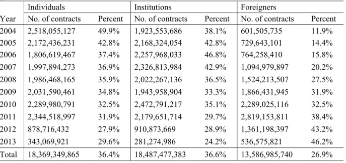
of total trading in the options market. Table 1 shows trading volumes in the KOSPI 200 options market by three investor types: domestic individuals, domestic institutions, and foreigners. Though the portion of trading volume by domestic individual investors has decreased over time, it still explains more than one-third of total trading volume for our sample period. The significant portion of individual investors in the KOSPI 200 options market indicates that the market is quite speculative and oriented toward short-term profit-seeking. Meanwhile, the continuously increasing portion of foreign participants in the KOSPI 200 options market reflects the openness and gradual matureness of the Korean market.

[Table 1 here]

The unique features of the KOSPI 200 options market motivate us to examine the statistical properties of the VKOSPI derived from the option prices. The active participation of individual investors implies that the dynamics of option prices and the derived implied volatility is more likely to be affected by market sentiment and behavioral factors, suggesting the importance of VKOSPI as a fear-gauge measure. The market openness of the KOSPI 200 options market and the great interest of foreign investors in this options market increase the possibility that the dynamics of VKOSPI is heavily dependent on global financial and macroeconomic shocks. Considering that most of foreign participants in the Korean financial markets are US financial institutions, it is important to consider the potential influence of US market shocks or volatilities to better understand the process and dynamics of VKOSPI.

The KOSPI 200 options market, which determines the activity and trading behavior of the VKOSPI level, is classified as a purely order-driven market which operates without the intermediation of designated market makers. All orders submitted by option traders are transacted through the centralized electronic limit order book (CLOB) based on the price and time priority rules. The CLOB transparently shows the current market liquidity (i.e., bid/ask spread and market depth), but, guarantees the anonymity of investors submitting orders. On a normal trading day, the options market opens at 09:00 and closes at 15:15. During the last 10 minutes (from 15:05 to 15:15) and during the hour long pre-opening session (from 08:00 to 09:00), standing orders are transacted under the uniform pricing rule. For remaining intraday periods (from 09:00 to 15:05), depending on whether they are market orders or limit orders, the submitted orders are immediately traded or consolidated into the CLOB to match with incoming orders. Four different options contracts with varying maturities can be traded each day. The maturity dates are the second Thursdays of three consecutive near-term months and one month nearest to each quarterly cycle (March, June, September, or December). However, among the four contracts, only the nearest maturity contracts are actively traded. The other three

longer-term contracts are rarely traded. The basic quoting unit of the KOSPI 200 options market is the “point.” One point corresponds to 100,000 Korean Won (KRW).2

With the great success of the KOSPI 200 options market, the KRX decided to publish the Korea’s model-free implied volatility index, VKOSPI, in April 2009. The VKOSPI presents the volatility of one-month-ahead KOSPI 200 underlying spot index. The VKOSPI value is determined by the expectation and sentiments of investors in the stock and options markets, and it reflects the fear and expectation of market participants. Based on the “fair variance swap” approach (Britten-Jones and Neuberger, 2000; Jiang and Tian, 2007), the VKOSPI value is calculated by using market prices of the nearest maturity and second nearest maturity KOSPI 200 options. This approach is similarly used to calculate the model-free VIX of the US market. The following mathematical equations, Equations (1)-(7), demonstrate how the VKOSPI can be derived from the historical time-series price data on the KOSPI 200 options and the underlying spot index.

VKOSPI 100 T σ NT N NT NT T σ N NT NT NT N N (1) σ T ∑ ∆K K e T Q K T F K 1 (2) σ _T ∑ ∆K K e T Q K T F K 1 (3) F S e T _{C P (4)} F S e T _{C P (5)} T NT N (6) T _NNT (7)

Equation (1) yields the annualized VKOSPI value, using the calculated values from Equations (2)-(7). In the above equations, N30 and N365 denote the numbers of days and of years per month, respectively.

and are the numbers of days remaining until the nearest maturity date and until the second nearest maturity date, respectively. r denotes the continuously compounded risk-free interest rate calculated from the CD (Certificate of Deposit) rate. K0 denotes the strike price closest to the

underlying KOSPI 200 spot index among strike prices equal to or lower than the spot index. For the KOSPI 200 call (put) options, Ki is the i-th highest (lowest) strike price compared to the level of K0. S1

(S2) denotes the strike price with the least difference between the nearest maturity (second nearest

maturity) call and put option prices. C1 (P1) is the price of the nearest maturity call (put) option; and

2 _{The microstructure of the KOSPI 200 options market is well documented in Ahn et al. (2008, 2010),}

C2 (P2) is the price of the second nearest maturity call (put) option. Equations (2) and (3) describe the

fluctuations of the nearest and second nearest maturity option contracts, respectively.

The VKOSPI value is directly affected by KOSPI 200 option prices, which reflect market sentiment, investor fear, and prevalent speculative trading motive. The KOSPI 200 options product is the representative index derivatives asset and its price dynamics critically depends on macroeconomic shocks and market-wide information. Therefore, the VKOSPI is sensitive to changes in the expectations and sentiment of market participants and immediately reflects public news and overseas shocks, which necessitates the consideration of US market shocks when examining the dynamics of VKOSPI.

3

Data and Sample Period

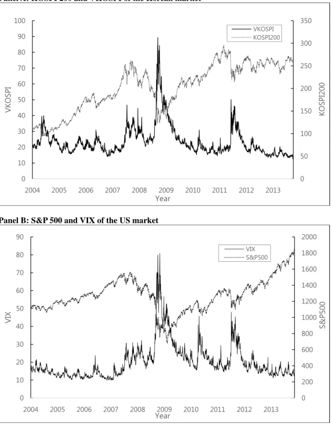
Although the VKOSPI is published since April 13, 2009, historical implied volatility index series can be constructed in the same manner as VKOSPI, which is introduced in the previous section. The volatility index series, which is constructed using option prices before the publication of VKOSPI, is also model-free and reflects the fear and sentiment of KOSPI 200 options traders. Since a sufficient number of traded options are needed to calculate volatility index values, we consider only post-2004 data. This is because the number of options classified by strike prices was not sufficient enough for deriving VKOSPI and the second nearest maturity options were infrequently traded until the mid-2000s. Our final sample data covers all daily observations of VKOSPI, KOSPI 200 spot index, VIX, S&P 500 spot index, and Korea’s macroeconomic variables (i.e., USD/KRW exchange rate returns, interest rates, credit spreads, and term spreads) from March 26, 2004 to Dec 30, 2013, which includes the recent global financial crisis period.3 Figure 1 plots the spot and implied volatility indices used in this study. Panel A presents the movements of KOSPI 200 spot index and VKOSPI, while Panel B presents the movements of S&P 500 spot index and VIX. Both implied volatility indexes capture the major financial and macroeconomic events resulting in a significant stock market decline. Especially, we can observe that, at the beginning of the recent global financial crisis, VIX and VKOSPI are at their highest levels during the sample period.

[Figure 1 here]

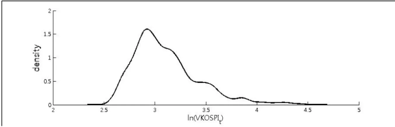
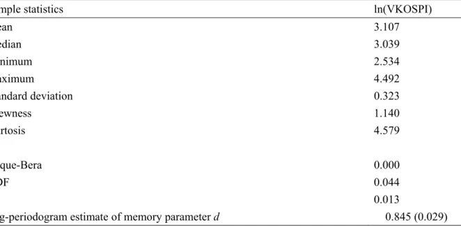
Table 2 presents the descriptive statistics of the logarithm of VKOSPI (ln(VKOSPIt)). The sample statistics in Table 2 and sample distribution of ln(VKOSPIt) shown in Figure 2 indicate that the

3 _{Instead of using data on the US and Korean spot markets, we have also tested our models using the}

dataset on index futures (i.e., the KOSPI 200 and the S&P 500 futures), which are tradable assets, and obtain qualitatively similar results. The results are available upon request.

ln(VKOSPIt) is skewed to the right and fat-tailed compared to the normal distribution. Table 2 also reports unit root test results for the time-series of ln(VKOSPIt). Both the Augmented Dickey-Fuller (ADF) and Phillips-Perron (PP) tests reject the null hypothesis of unit root at the 5% significance level, which indicates that the ln(VKOSPIt) series is not a unit root process. Meanwhile, the log-periodogram estimate of memory parameter d is 0.845 and its standard error is 0.029 for the ln(VKOSPIt) series, suggesting that the historical time-series of ln(VKOSPIt) is characterized by a long memory process.

[Table 2 here] [Figure 2 here]

4 Methodological

Considerations

4.1 Estimated

Models

As the results in Table 2 present that the time-series logarithm value of ln(VKOSPIt) is shown to be a long memory process while it is not a unit root process, we adopt the heterogeneous autoregressive (HAR) framework of Corsi (2009), as in Fernandes et al. (2014), and modified it. For realized volatility measure at time t, RVt, the pure HAR model is defined as:

RVt =β0 +β1RVt-1 + β3RV(w)t-1 +β3 RV(m)t-1+εt, whereRV(w)

t-1=(1/5)∑5i=1 RVt-i and RV(m)t-1=(1/22)∑22i=1 RVt-i. (8)

In Equation (8), RV(w)

tand RV(m)t represent medium-term weekly (w) realized volatility and long-term monthly (m) realized volatility at time t, respectively. The key motivation of including these heterogeneous components is that agents with different time horizons perceive, react to, and cause different types of volatility components. Corsi (2009) finds that the heterogeneous components have important effects in reproducing the long memory property and that that the empirical performance of the HAR model is comparable to the ARFIMA model, which has been typically adopted to model and forecast long memory time series.

For yt = ln(VKOSPIt), the pure HAR model can be written as:

yt = Xt-1β+ut, whereXt=[1 y1,ty5,ty10,ty22,t] for yh,t= ∑ . (9)

While Fernandes et al. (2014) also include the quarterly component y66,t for modeling the dynamics of VIX, we exclude it because the component is found insignificant for modeling the dynamics of

VKOSPI index. This reflects the dominance of short-term traders and speculative individual investors in the KOSPI 200 options market. By incorporating financial and macroeconomic variables into the HAR framework, the HAR-X model is constructed as follows:

yt = Xt-1β+Zt-1γ+ut (10)

where Zt=[z1t z2t … zkt] is a k-dimensional vector of explanatory variables. By including relevant macro-finance variables as Zt, the HAR-X model is expected to be improved in terms of both in-sample and out-of-in-sample performances, if the incorporated exogenous variables are helpful to describe the VKOSPI dynamics.

We consider the following macro-finance variables of the Korean market as exogenous variables: i) the log return of USD/KRW exchange rate, ii) the 3-month CD rate, which is a proxy for Korea’s risk-free interest rate, iii) the yield difference between BBB and AA corporate bonds in Korea, which measures the credit spread, iv) the difference between the yields on the 5-year government bond and 3-month CD rates in Korea, which measures the term spread, and v) the log return of the KOSPI 200 index, which captures shocks in the underlying spot market. We also consider some US financial market variables, which is the most influential overseas market, to investigate the effect of US shocks and news on the dynamics of VKOSPI. The US market shocks are measured by return (i.e. S&P 500 index) and risk (i.e. VIX). Unlike the framework of Fernandes et al. (2014), we include lagged regressors Zt-1, instead of the contemporaneous regressors Zt, in the HAR-X model in order to avoid possible endogeneity problems. Besides, such lag structure is more suitable because one of the main purposes of this paper is to measure the out-of-sample forecasting performance of our models.

4.2

Forecasting Procedure and Evaluation Criteria

To obtain out-of-sample forecasts for future ln(VKOSPIt), we adopt the rolling window forecast procedure with moving windows of four years (1,008 trading days). We obtain one-step ahead out-of-sample forecasts (h=1) and multi-step ahead out-of-sample forecasts (h= 5, 10, and 22) for all models. The number of forecasts are 1400, 1396, 1391, and 1379, respectively, for h=1, 5, 10, and 22. The forecast period for the one-step ahead out-of-sample forecast is from May 23, 2008 to December 30, 2013. For multi-step ahead forecasting, we adopt a direct forecasting procedure: To compute h-day ahead forecasts, we replace yt with yt+h-1 in the models. This allows us to produce multi-step ahead

forecasts without imposing any assumption about future realizations of the explanatory variables. To evaluate the predictive power, we use the mean squared error (MSE) and mean absolute error (MAE) loss function. We calculate the difference in MSE or MAE losses between two models as follows:

dt= L(yt,benchmark, yt) – L(yt,0, yt) (11)

where yt,benchmark denotes the forecast of the benchmark model, yt,0 denotes the forecast of the key

model, and L(yt,benchmark, yt) and L(yt,0, yt) are forecast losses measured based on MSE or MAE. If the distance, dt, is positive, we can conclude that the key model outperforms the benchmark model in that it has a smaller loss.

The significance of any difference in the loss is tested using the Diebold-Mariano and West (henceforth DMW) test (Diebold-Mariano (1995); West (1996)). The DMW statistics are calculated using the difference in the losses of two models as follows:

(12)

where dT denotes the sample mean of dt and TF is the number of forecasts. avar(.) operator calculates the asymptotic variance. The asymptotic variance of the average is computed using a Newey-West variance estimator with the number of lags set to TF1/3. The asymptotic distribution of the test statistic is the standard normal.

5 Empirical

Findings

We estimate the pure HAR model and the various versions of HAR-X model with different exogenous variables. To avoid possible multicollinearity problem, we design the following procedure and choose seven alternative models (models M1-M7) based on the significance of estimated coefficients. In the first step, we estimate the pure HAR model given by Equation (8) and remove insignificant coefficient terms, which leads to Model 1 (M1). The estimation result of the pure HAR model yields that only the biweekly component, y10,t, is statistically significantly, so we only add this component into M1. In the second step, we estimate HAR-X model using four macro variables, which are USD/KRW exchange rate return (Ex) , interest rate (Interest rate), credit spread (Credit spread), and term spread (Term spread), and choose Model 2 (M2) by removing variables with insignificant coefficients. In the third step, we incorporate each financial variable related to the US or Korean market, which is the logarithm of US implied volatility index measured by VIX (ln(VIX)), the US stock market return measured by S&P 500 spot return (returnUS_{), or the Korean stock market return measured by KOSPI} 200 spot return (returnKOR_{) and these variables are added to the model in the second step. By} removing variables with insignificant coefficients, we obtain Model 3 (M3), Model 4 (M4), and Model 5 (M5). At this stage, only statistically significant terms, namely, y1,t, y5,t, y10,t, y22,t, and Korea’s macroeconomic variables are included. In the fourth step, we add both ln(VIX) and returnUS _{to the}

model in the second step, which leads to Model 6 (M6). In the fifth step, we add both ln(VIX) and returnKOR _{to the model in the second step, which leads to Model 7 (M7). The joint presence of residual} autocorrelation and lagged dependent variable among the regressors induces inconsistent coefficient estimates. Therefore, in each case we ensure that residual is not serially correlated by adding lagged dependent variables in the model up to lag k (k=1,5, and 10). Consequently, the following seven models (M1-M7) are estimated.

M1: yt = β0 + β1y1,t + β2y10,t+εt

M2: yt = β0 + β1y1,t + β2y10,t+γ1Ext-1+γ2Interest ratet-1+γ3Credit spreadt-1+γ4Term spreadt-1+εt M3: yt = β0 + β1y1,t + β2y5,t+γ1Ext-1+γ2ln(VIXt-1) +εt

M4: yt = β0 + β1y1,t + β2y10,t+γ1Interest ratet-1+γ2Credit spreadt-1+γ3returnUSt-1+εt

M5: yt = β0 + β1y1,t + β2y10,t + γ1Ext-1 + γ2Interest ratet-1 + γ3Credit spreadt-1 + γ4Term spreadt-1 +

γ5returnKORt-1 + εt

M6: yt = β0 + β1y1,t + β2y10,t+γ1Interest ratet-1+ γ2ln(VIXt-1) + γ3returnUSt-1+εt

M7: yt = β0 + β1y1,t + β2y5,t+γ1Ext-1+ γ2ln(VIXt-1) + γ3returnKORt-1+εt (13)

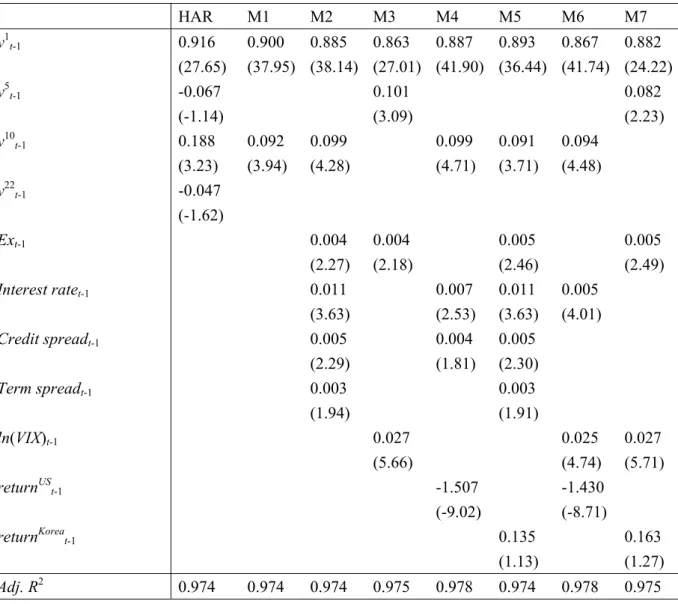
Table 3 reports the least squares estimates of the model coefficients and their t-statistics based on heteroskedasticity-consistent standard errors. For each model, the adjusted R2 value is also reported to measure the in-sample fitting performance. For the pure HAR model, the coefficients of daily and biweekly components, y1,t-1 and y10,t-1, are significantly estimated at the 1% significance level while

the weekly and monthly components, y5,t-1 and y22,t-1, are insignificant. When we conduct the Wald

test, y5,t-1 and y22,t-1 are also jointly insignificant. If the quarterly component y66,t-1 is included as an

explanatory variable as in Fernandes et al. (2014), y5,t-1, y22,t-1, and y66,t-1 are insignificant at the 5%

significance level and also jointly insignificant according to the Wald test. Therefore, we remove insignificant terms and leave only y1,t-1 and y10,t-1 terms in the model and denote it by M1. These

results are different from those in Fernandes et al. (2014), which report that the estimated coefficient for y66,t-1 is significant for the VIX index. This reflects the relatively higher participation of domestic

individual investors who are short-term oriented with speculative motives compared to their institutional counterparts in the KOSPI 200 options market, which reduces the medium- or long-term predictability of VKOSPI.

[Table 3 here]

When the four macro variables are added to the model, y5,t-1 and y22,t-1 are still insignificant while

appreciation of Korea’s currency (KRW) and an increase in the variables of the interest rate, credit spread, and term spread are associated with a higher VKOSPI level. In M3, when the US implied volatility index, VIX, is included, among the four macroeconomic variables, only the exchange rate returns remains significant. The lagged VIX index is positively related to the VKOSPI level, which is quite plausible considering that the VIX index captures market-wide volatility. We find that the US stock market returns are significantly and negatively related to the future VKOSPI (see M4) whereas the Korean stock market returns are not significantly related to the one-step ahead VKOSPI after controlling the macroeconomic variables (see M5). This means that the influence of the KOSPI 200 stock market return on the VKOSPI is mostly explained by the macroeconomic variables and that the Korea’s stock market return is redundant for describing the dynamics of VKOSPI if the macroeconomic factors are considered. The finding that the VKOSPI is not predicted by its underlying stock market return, but by the overseas stock market returns is interesting in that it provides a skeptical view on previous literature’s attempts to focus on the return-volatility relationship within a closed-economy context. Further, our finding on the relationship between VKOSPI and lagged S&P 500 return is consistent with an asymmetric volatility response, which indicates that the stock market return negatively affects the volatility level (Bekaert and Wu, 2000; Wu, 2001; Han et al., 2012; Lee and Ryu, 2013). Based on the adjusted R2 values and the significance of estimated coefficients, we find that the HAR-X model incorporating both US stock market return and implied volatility exhibits the best in-sample fitting performance and absorb most of the explanatory power of other macroeconomic variables in describing the VKOSPI dynamics (see M6) whereas the stock market return loses its explanatory power when it is replaced by the Korean stock market return and the adjusted R2 _{values of the model with the Korean stock market return decreases (see M7).}

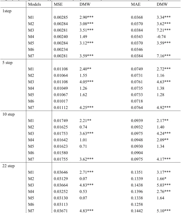
Table 4 reports out-of-sample forecast results. We report MSEs and MAEs of the seven versions of HAR-X model (M1-M7) for one-step and multi-step ahead out-of-sample forecasts (h=1, 5, 10, and 22). We observe that M6 outperforms the rest of the models by exhibiting the lowest MSE and MAE losses in almost all cases, suggesting that M6 is the best model in out-of-sample forecasting as well as in-sample fitting. For one-step ahead forecasting, the DMW test between M6 and each model, except for M4, rejects the null hypothesis of equal predictability. This implies that M6 produces significantly better one-step ahead out-of-sample forecast. Exceptionally, M4 has the lowest MAE while the DMW tests between M6 and M4 are insignificant in both MSE and MAE. If we exclude M6, M4 has the lowest MSE value. This implies that the stock return of the US market plays an important role in one-day ahead out-of-sample forecasting of VKOSPI. Regarding the multi-step ahead forecasting, the M6 model has the lowest MSE and MAE losses in all cases and the DMW test rejects the null hypothesis of equal predictability in some cases. For 10-step and 22-step ahead forecasting, the DMW test statistics, in terms of MAE, between M6 and M4 are significant at the 5% or 1% level, which implies

that Model 6 produces significantly better forecasts than M4. This indicates that the inclusion of VIX is helpful particularly for long-term forecasting of VKOSPI.

[Table 4 here]

When we compare M6 with M1, M6 provides better out-of-sample forecasts than M1 in both MSE and MAE losses and for all forecast horizons. The DMW test between these two models rejects the null hypothesis of equal predictability for all cases at the 5% or 1% significance level. This result is interesting and contrasts with Fernandes et al. (2014) who report that the pure HAR model performs well and it is difficult to beat the pure HAR model in forecasting VIX. In their study, for example, in terms of MSE and MAE losses, the pure HAR model shows the best 1-step ahead forecast results. In contrast with their results, for the analysis on the VKOSPI, our chosen model, M6, clearly dominates the pure HAR model in our sample for forecasting all horizons.

As in within-sample estimation result, we confirm that the Korea’s stock market return is still redundant in forecasting future VKOSPI when other relevant covariates (the macroeconomic factors or VIX) are included. Comparing Model M2 with that of M5, their forecast errors (MSEs or MAEs) are similar to each other. This is because they produce similar out-of-sample forecasts for all horizons, which implies that the Korea’s stock market return is redundant in forecasting future VKOSPI when the macroeconomic factors are included. Comparing Model 3 with Model 7, their forecast errors are also similar to each other because each model produces similar forecasts for all horizons. The inclusion of the Korea’s stock market return does not make any significant contribution in forecasting future VKOSPI.

5

Conclusions and Policy Implications

Using the modified HAR framework, we analyze the statistical properties of an emerging market volatility index, namely the VKOSPI. Previous studies focus on advanced markets and do not consider the influence of overseas markets in predicting implied market volatility indexes. Our empirical results show that that the statistical properties of the VKOSPI are well captured by the HAR framework and that Korea’s macroeconomic variables can explain the VKOSPI dynamics. In particular, we find that the stock market return and implied volatility index of US market play a key role in explaining the dynamics of VKOSPI and predicting the future VKOSPI level, and their explanatory power dominates that of Korea’s macro-finance variables, which supports the consideration of the global information linkages when analyzing and modeling the implied volatility dynamics especially in emerging markets which are subject to significant global shocks.

Considering that the VKOSPI reflects market sentiment and the risk perspective of market participants, our study uncovering the time-series properties of the VKOSPI and explaining its dynamics provides useful trading information for market practitioners to implement investment strategies including hedging, speculative short-term trading, and broad portfolio management, based on the predicted implied volatility index. Our study on Korea and empirical findings for the VKOSPI can be extended to other emerging markets and provide a yardstick for comparison and contrasting of findings.

Acknowledgements

The authors are grateful for helpful comments and suggestions from Robert I. Webb, Heejin Yang, and the participants at the 2014 Sungkyunkwan University (SKKU) economics seminar.

References

[1] Ahn, H-.J., J. Kang, and D. Ryu (2008). Informed trading in the index option market: The case of KOSPI 200 options, Journal of Futures Markets 28(12): 1118-1146.

http://onlinelibrary.wiley.com/doi/10.1002/fut.20369/pdf

[2] Ahn, H-.J., J. Kang, and D. Ryu (2010). Information effects of trade size and trade direction: Evidence from the KOSPI 200 index options market, Asia-Pacific Journal of Financial Studies 39(3): 301-339.

http://onlinelibrary.wiley.com/doi/10.1111/j.2041-6156.2010.01016.x/pdf

[3] Banerjee, P.S., J.S. Doran, and D.R. Peterson (2007). Implied volatility and future portfolio returns, Journal of Banking and Finance 31(10): 3183-3199.

http://www.sciencedirect.com/science/article/pii/S0378426607000490#

[4] Becker, R., A.E. Clements, and S.I. White (2007). Does implied volatility provide any information beyond that captured in model-based volatility forecasts?, Journal of Banking and Finance 31(8): 2535-2549.

http://www.sciencedirect.com/science/article/pii/S0378426607000428

[5] Bekaert, G. and G. Wu (2000). Asymmetric Volatility and Risk in Equity Markets, Review of Financial Studies 13(1): 1-42.

[6] Blair, B.J., S.H. Poon, and S.J. Taylor (2001). Forecasting S&P 100 volatility: The incremental information content of implied volatilities and high-frequency index returns, Journal of

Econometrics 105(1): 5-26.

http://www.sciencedirect.com/science/article/pii/S0304407601000689

[7] Britten-Jones, M., and A. Neuberger (2000). Option Prices, Implied Price Processes, and Stochastic Volatility, Journal of Finance 55(2): 839-866.

http://onlinelibrary.wiley.com/doi/10.1111/0022-1082.00228/abstract

[8] Carr, P., and L. Wu (2006). A Tale of Two Indices, Journal of Derivatives 13(3): 13-29. http://papers.ssrn.com/sol3/papers.cfm?abstract_id=871729

[9] Chae, J., and E.J. Lee (2011). An analysis of split orders in an index options market, Applied Economics Letters 18(5): 473-477.

http://www.tandfonline.com/doi/abs/10.1080/13504851003724200#.VMok6Xn9mmQ

[10] Corrado, C.J., and T.W. Miller (2005). The forecast quality of CBOE implied volatility indexes, Journal of Futures Markets 25(4): 339-373.

http://onlinelibrary.wiley.com/doi/10.1002/fut.20148/pdf

[11] Corsi, F. (2009). A simple approximate long memory model of realized volatility, Journal of Financial Econometrics 7(2): 174-196.

http://papers.ssrn.com/sol3/papers.cfm?abstract_id=626064

[12] Demeterfi, K., E. Derman, M. Kamal, and J. Zou (1999). A Guide to Volatility and Variance Swaps, Journal of Derivatives 6(4): 9-32.

http://www.iijournals.com/doi/abs/10.3905/jod.1999.319129

[13] Diebold, F.X., and R.S. Mariano (1995). Comparing predictive accuracy, Journal of Business and Economic Statistics, 13(3): 253-263.

http://amstat.tandfonline.com/doi/abs/10.1080/07350015.1995.10524599#.VMor5Hn9mmQ [14] Eom, K.S., and S.B. Hahn (2005). Traders' strategic behavior in an index options market, Journal

of Futures Markets 25(2): 105–133.

[15] Fernandes, M., M.C. Medeiros, and M. Scharth (2014). Modeling and predicting the CBOE market volatility index, Journal of Banking & Finance 40(March): 1-10.

http://www.sciencedirect.com/science/article/pii/S0378426613004172#

[16] Frijns, B., C. Tallau, and A. Tourani-Rad (2010). The information content of implied volatility: Evidence from Australia, Journal of Futures Markets 30(2): 134-155.

http://onlinelibrary.wiley.com/doi/10.1002/fut.20405/pdf

[17] Giot, P. (2005). Implied volatility indexes and daily Value at Risk models, Journal of Derivatives 12(4): 54-64.

http://www.iijournals.com/doi/abs/10.3905/jod.2005.517186

[18] Giot, P., and S. Laurent (2007). The information content of implied volatility in light of the jump/continuous decomposition of realized volatility, Journal of Futures Markets 27(4): 337-359. http://onlinelibrary.wiley.com/doi/10.1002/fut.20251/pdf

[19] Guo, B., Q. Han, and D. Ryu (2013). Is KOSPI 200 options market efficient? Parametric and nonparametric tests of martingale restriction, Journal of Futures Markets 33(7): 629-652. http://onlinelibrary.wiley.com/doi/10.1002/fut.21563/full

[20] Han, Q., B. Guo, D. Ryu, and R.I. Webb (2012). Asymmetric and negative return-volatility relationship: The case of the VKOSPI, Investment Analysts Journal 76(November): 69-78. http://www.economics-ejournal.org/economics/journalarticles/2013-3/references/HanEtAl2012 [21] Jiang, G.J., and Y.S. Tian (2007). Extracting model-free volatility from option prices: An

examination of the VIX index, Journal of Derivatives 14(3): 35-60. http://www.iijournals.com/doi/abs/10.3905/jod.2007.681813

[22] Kim, H., and D. Ryu (2012). Which trader’s order-splitting strategy is effective? The case of an index options market, Applied Economics Letters 19(17): 1683-1692.

http://www.tandfonline.com/doi/abs/10.1080/13504851.2012.665590#.VMoveXn9mmQ

[23] Kim, J.S., and D. Ryu (2015). Are the KOSPI 200 Implied Volatilities Useful in Value-at-Risk Models?, Emerging Markets Review 22(March): 43-64.

[24] Konstantinidi, E., G. Skiadopoulos, and E. Tzagkaraki (2008). Can the evolution of implied volatility be forecasted? Evidence from European and US implied volatility indices, Journal of Banking & Finance 32(11): 2401-2411.

http://www.sciencedirect.com/science/article/pii/S0378426608000526

[25] Lee, B.S., and D. Ryu (2013). Stock returns and implied volatility: A new VAR approach, Economics:The Open-Access, Open-Assessment E-Journal 7(2013-3): 1-20.

http://www.economics-ejournal.org/economics/journalarticles/2013-3

[26] Lee, C., and D. Ryu (2014). The volatility index and style rotation: Evidence from the Korean stock market and VKOSPI, Investment Analysts Journal 79(May): 29-39.

http://www.journals4free.com/link.jsp?l=4662775

[27] Poteshman, A.M. (2000). Forecasting future volatility from option prices, working paper, University of Illinois at Urbana-Champaign, Urbana-Champaign, IL.

http://papers.ssrn.com/sol3/papers.cfm?abstract_id=243151

[28] Ryu, D. (2011). Intraday price formation and bid-ask spread components: A new approach using a cross-market model, Journal of Futures Markets 31(12): 1142-1169.

http://onlinelibrary.wiley.com/doi/10.1002/fut.20533/pdf

[29] Ryu, D. (2012). Implied volatility index of KOSPI200: Information contents and properties, Emerging Markets Finance and Trade 48(S2): 24-39.

http://www.tandfonline.com/doi/abs/10.2753/REE1540-496X48S202#.VMozM3n9mmQ

[30] Ryu, D. (2015). The information content of trades: An analysis of KOSPI 200 index derivatives, Journal of Futures Markets 35(3): 201-221.

http://onlinelibrary.wiley.com/doi/10.1002/fut.21637/pdf

[31] Ryu, D., J. Kang, and S. Suh (2015). Implied pricing kernels: An alternative approach for option valuation, Journal of Futures Markets 35(2): 127-147.

http://onlinelibrary.wiley.com/doi/10.1002/fut.21618/full

[32] Simon, D.P. (2003). The Nasdaq volatility index during and after the bubble, Journal of Derivatives 11(2): 9-24.

http://www.iijournals.com/doi/abs/10.3905/jod.2003.319213

[33] Taylor, S.J., P.K. Yadav, and Y. Zhang (2010). Information Content of Implied Volatilities and Model-Free Volatility Expectations: Evidence from Options Written on Individual Stocks, Journal of Banking & Finance 34(4): 871-881.

http://www.sciencedirect.com/science/article/pii/S0378426609002489#

[34] West, K.D. (1996). Asymptotic inference about predictive ability, Econometrica 64(5) 1067-1084. http://www.jstor.org/stable/2171956?seq=1#page_scan_tab_contents

[35] Wu, G. (2001). The Determinants of Asymmetric Volatility, Review of Financial Studies 14(3): 837-859.

Figure 1: Time trends of stock market returns and implied volatility indices

Notes: The two panels of this figure show the time-trends of the stock market returns and implied volatility indices for the Korean (Panel A) and US (Panel B) markets, respectively. In each panel, the left-hand vertical axis denotes the percentage value of each implied volatility index and the right-hand vertical axis denotes the level of each stock market return.

Panel A: KOSPI 200 and VKOSPI of the Korean market

Panel B: S&P 500 and VIX of the US market

0 50 100 150 200 250 300 350 0 10 20 30 40 50 60 70 80 90 100 2004 2005 2006 2007 2008 2009 2010 2011 2012 2013 KOSPI200 VKOSPI Year VKOSPI KOSPI200 0 200 400 600 800 1000 1200 1400 1600 1800 2000 0 10 20 30 40 50 60 70 80 90 2004 2005 2006 2007 2008 2009 2010 2011 2012 2013 S&P500 VIX Year VIX S&P500

Figure 2: Kernel density estimate of the logarithm of VKOPI

Notes: This figure presents the kernel density estimate of the logarithm of VKOSPI (ln(VKOSPIt)). The Gaussian kernel function is used in estimating the kernel density.

Table 1: Trading volume by investor types

Notes: This table presents the trend of trading volume of KOSPI 200 options by three investor types which are domestic individuals (Individuals), domestic institutions (Institutions), and foreigners (Foreigners), during the sample period (January 2003 to December 2013). The trading volume is presented in the number of options contracts (No. of contracts). Percent columns present the proportion of the trading volume of each investor type in percentage values. Source: Korea Exchange (www.krx.co.kr).

Individuals Institutions Foreigners

Year No. of contracts Percent No. of contracts Percent No. of contracts Percent

2004 2,518,055,127 49.9% 1,923,553,686 38.1% 601,505,735 11.9% 2005 2,172,436,231 42.8% 2,168,324,054 42.8% 729,643,101 14.4% 2006 1,806,619,467 37.4% 2,257,968,033 46.8% 764,258,410 15.8% 2007 1,997,894,273 36.9% 2,326,813,984 42.9% 1,094,979,897 20.2% 2008 1,986,468,165 35.9% 2,022,267,136 36.5% 1,524,213,507 27.5% 2009 2,031,590,461 34.8% 1,943,958,904 33.3% 1,866,431,945 31.9% 2010 2,289,980,791 32.5% 2,472,791,217 35.1% 2,289,025,116 32.5% 2011 2,344,518,997 31.9% 2,179,651,714 29.7% 2,819,153,811 38.4% 2012 878,716,432 27.9% 910,873,669 28.9% 1,361,198,397 43.2% 2013 343,069,921 29.6% 281,274,986 24.2% 536,575,821 46.2% Total 18,369,349,865 36.4% 18,487,477,383 36.6% 13,586,985,740 26.9%

Table 2: Descriptive statistics for the logarithm of the VKOSPI index

Notes: The sample period spans from March 26, 2004 to December 30, 2013, which includes 2,430 daily observations. This table reports the sample mean, median, minimum, maximum, standard deviation, skewness, and kurtosis values of the logarithm of the VKOSPI index, as well as the p -values of Jarque-Bera test for normality and of Augmented Dickey-Fuller (ADF) and Phillips-Perron (PP) tests for unit roots. Finally, we also report the log-periodogram estimate of the memory parameter d with its standard error in parenthesis.

Sample statistics ln(VKOSPI)

Mean 3.107 Median 3.039 Minimum 2.534 Maximum 4.492 Standard deviation 0.323 Skewness 1.140 Kurtosis 4.579 Jarque-Bera 0.000 ADF 0.044 PP 0.013

Table 3: Estimation results of the pure HAR model and the HAR-X model: In-sample model fitness

Notes: This table shows the in-sample fitness of the pure HAR model (HAR) and its extended HAR model (HAR-X) with exogenous variables (models M1-M7). yth denotes the average value of the logarithm of VKOSPI over the last h days. Ext-1 is the log return of USD/KRW (US Dollar/Korean

Won) exchange rate at time t-1 (positive Ext-1 value means that Korean Won (KRW) appreciates).

Interest rate denotes the 3-month CD rates. Credit spread is the yield difference between BBB and AA corporate bonds. Term spread is calculated as the difference between the yields on the 5-year government bonds and the 3-month CD rates. ln(VIX) is the logarithm of VIX. returnUS _{is the log} return of S&P 500 index and returnKorea _{is the log return of KOSPI 200 index. The table reports the} least squares estimates of the coefficients and their t-statistics provided in parentheses are based on heteroskedasticity-consistent standard errors. The last row shows the adjusted R² (Adj. R2_{) for each}

model. HAR M1 M2 M3 M4 M5 M6 M7 y1 t-1 0.916 0.900 0.885 0.863 0.887 0.893 0.867 0.882 (27.65) (37.95) (38.14) (27.01) (41.90) (36.44) (41.74) (24.22) y5 t-1 -0.067 0.101 0.082 (-1.14) (3.09) (2.23) y10 t-1 0.188 0.092 0.099 0.099 0.091 0.094 (3.23) (3.94) (4.28) (4.71) (3.71) (4.48) y22t-1 -0.047 (-1.62) Ext-1 0.004 0.004 0.005 0.005 (2.27) (2.18) (2.46) (2.49) Interest ratet-1 0.011 0.007 0.011 0.005 (3.63) (2.53) (3.63) (4.01) Credit spreadt-1 0.005 0.004 0.005 (2.29) (1.81) (2.30) Term spreadt-1 0.003 0.003 (1.94) (1.91) ln(VIX)t-1 0.027 0.025 0.027 (5.66) (4.74) (5.71) returnUS t-1 -1.507 -1.430 (-9.02) (-8.71) returnKorea t-1 0.135 0.163 (1.13) (1.27) Adj.R2 _{0.974 0.974 0.974 0.975 0.978 0.974 0.978 0.975}

Table 4: Out-of-sample forecast evaluation of the HAR-X model (M1-M7)

Notes: This table shows out-of-sample forecasting performance of the HAR model (HAR-X) with exogenous variables (models M1-M7). MSE denotes the mean squared errors and MAE is the mean absolute errors. DMW presents Diebold-Mariano and West (DMW) test statistics. DMW test statistic is calculated from the distance between M6 (the key model) and the rest models. *, **, and *** signify rejecting the null hypothesis of equal predictability for 10%, 5%, and 1%, respectively.

Models MSE DMW MAE DMW

1step M1 0.00285 2.90*** 0.0368 3.34*** M2 0.00284 3.08*** 0.0370 3.62*** M3 0.00281 3.51*** 0.0384 7.21*** M4 0.00240 1.49 0.0343 -0.74 M5 0.00284 3.12*** 0.0370 3.59*** M6 0.00234 0.0346 M7 0.00281 3.59*** 0.0384 7.16*** 5 step M1 0.01108 2.40** 0.0749 2.72*** M2 0.01064 1.55 0.0731 1.16 M3 0.01108 4.05*** 0.0761 4.63*** M4 0.01049 1.26 0.0735 1.38 M5 0.01067 1.62 0.0733 1.28 M6 0.01017 0.0718 M7 0.01112 4.25*** 0.0764 4.92*** 10 step M1 0.01749 2.21** 0.0939 2.17** M2 0.01625 0.74 0.0932 1.40 M3 0.01753 3.63*** 0.0975 4.24*** M4 0.01642 1.01 0.0948 2.09** M5 0.01623 0.71 0.0930 1.34 M6 0.01580 0.0904 M7 0.01755 3.62*** 0.0975 4.17*** 22 step M1 0.03646 2.71*** 0.1351 3.17*** M2 0.03129 0.07 0.1339 1.66* M3 0.03664 4.83*** 0.1438 5.03*** M4 0.03252 0.53 0.1396 2.76*** M5 0.03130 0.07 0.1338 1.64 M6 0.03113 0.1258 M7 0.03671 4.83*** 0.1442 5.10***

Please note:

You are most sincerely encouraged to participate in the open assessment of this discussion paper. You can do so by either recommending the paper or by posting your comments.

Please go to:

http://www.economics-ejournal.org/economics/discussionpapers/2015-7

The Editor