By Davis Yen Pan
Abstract
Compared to most digital data types, with the exception of digital video, the data rates associ-ated with uncompressed digital audio are substan-tial. Digital audio compression enables more effi-cient storage and transmission of audio data. The many forms of audio compression techniques offer a range of encoder and decoder complexity, compressed audio quality, and differing amounts of data com-pression. The -law transformation and ADPCM coder are simple approaches with low-complexity, low-compression, and medium audio quality algo-rithms. The MPEG/audio standard is a high-complexity, high-compression, and high audio qual-ity algorithm. These techniques apply to general au-dio signals and are not specifically tuned for speech signals.
Introduction
Digital audio compression allows the efficient stor-age and transmission of audio data. The various au-dio compression techniques offer different levels of complexity, compressed audio quality, and amount of data compression.
This paper is a survey of techniques used to com-press digital audio signals. Its intent is to provide useful information for readers of all levels of ex-perience with digital audio processing. The paper
begins with a summary of the basic audio digitiza-tion process. The next two secdigitiza-tions present detailed descriptions of two relatively simple approaches to audio compression: -law and adaptive differential pulse code modulation. In the following section, the paper gives an overview of a third, much more so-phisticated, compression audio algorithm from the Motion Picture Experts Group. The topics covered in this section are quite complex and are intended for the reader who is familiar with digital signal processing. The paper concludes with a discussion of software-only real-time implementations.
Digital Audio Data
The digital representation of audio data offers many advantages: high noise immunity, stability, and reproducibility. Audio in digital form also al-lows the efficient implementation of many audio processing functions (e.g., mixing, filtering, and equalization) through the digital computer.
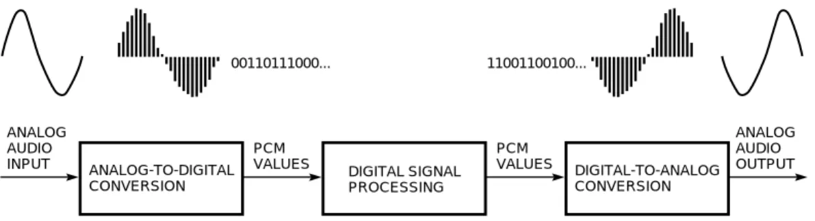
The conversion from the analog to the digital do-main begins by sampling the audio input in regular, discrete intervals of time and quantizing the sam-pled values into a discrete number of evenly spaced levels. The digital audio data consists of a sequence of binary values representing the number of quan-tizer levels for each audio sample. The method of representing each sample with an independent code word is called pulse code modulation (PCM). Figure 1 shows the digital audio process.
ANALOG-TO-DIGITAL
CONVERSION DIGITAL SIGNALPROCESSING
DIGITAL-TO-ANALOG CONVERSION PCM VALUES PCM VALUES ANALOG AUDIO INPUT ANALOG AUDIO OUTPUT 00110111000... 11001100100...
According to the Nyquist theory, a time-sampled signal can faithfully represent signals up to half the sampling rate.[1] Typical sampling rates range from 8 kilohertz (kHz) to 48 kHz. The 8-kHz rate covers a frequency range up to 4 kHz and so covers most of the frequencies produced by the human voice. The 48-kHz rate covers a frequency range up to 24 kHz and more than adequately covers the entire audi-ble frequency range, which for humans typically ex-tends to only 20 kHz. In practice, the frequency range is somewhat less than half the sampling rate because of the practical system limitations.
The number of quantizer levels is typically a power of 2 to make full use of a fixed number of bits per au-dio sample to represent the quantized values. With uniform quantizer step spacing, each additional bit has the potential of increasing the signal-to-noise ratio, or equivalently the dynamic range, of the quantized amplitude by roughly 6 decibels (dB). The typical number of bits per sample used for digital audio ranges from 8 to 16. The dynamic range ca-pability of these representations thus ranges from 48 to 96 dB, respectively. To put these ranges into perspective, if 0 dB represents the weakest audi-ble sound pressure level, then 25 dB is the mini-mum noise level in a typical recording studio, 35 dB is the noise level inside a quiet home, and 120 dB is the loudest level before discomfort begins.[2] In terms of audio perception, 1 dB is the minimum au-dible change in sound pressure level under the best conditions, and doubling the sound pressure level amounts to one perceptual step in loudness.
Compared to most digital data types (digital video excluded), the data rates associated with uncom-pressed digital audio are substantial. For example, the audio data on a compact disc (2 channels of au-dio sampled at 44.1 kHz with 16 bits per sample) re-quires a data rate of about 1.4 megabits per second. There is a clear need for some form of compression to enable the more efficient storage and transmis-sion of this data.
The many forms of audio compression techniques differ in the trade-offs between encoder and decoder complexity, the compressed audio quality, and the amount of data compression. The techniques pre-sented in the following sections of this paper cover the full range from the -law, a low-complexity, low-compression, and medium audio quality algo-rithm, to MPEG/audio, a complexity, high-compression, and high audio quality algorithm. These techniques apply to general audio signals and are not specifically tuned for speech signals. This paper does not cover audio compression algorithms designed specifically for speech signals. These al-gorithms are generally based on a modeling of the vocal tract and do not work well for nonspeech audio
signals.[3,4] The federal standards 1015 LPC (linear predictive coding) and 1016 CELP (coded excited lin-ear prediction) fall into this category of audio com-pression.
-law Audio Compression
The-law transformation is a basic audio compres-sion technique specified by the Comité Consultatif Internationale de Télégraphique et Téléphonique (CCITT) Recommendation G.711.[5] The transfor-mation is essentially logarithmic in nature and al-lows the 8 bits per sample output codes to cover a dynamic range equivalent to 14 bits of linearly quantized values. This transformation offers a com-pression ratio of (number of bits per source sample) /8 to 1. Unlike linear quantization, the logarithmic step spacings represent low-amplitude audio sam-ples with greater accuracy than higher-amplitude values. Thus the signal-to-noise ratio of the trans-formed output is more uniform over the range of amplitudes of the input signal. The-law transfor-mation is y = 2550 127 ln(1+)2 ln(1 + jxj) for x 0 1270 127 ln(1+)2 ln(1 + jxj) for x < 0
where m = 255, and x is the value of the input sig-nal normalized to have a maximum value of 1. The CCITT Recommendation G.711 also specifies a simi-lar A-law transformation. The-law transformation is in common use in North America and Japan for the Integrated Services Digital Network (ISDN) 8-kHz-sampled, voice-grade, digital telephony service, and the A-law transformation is used elsewhere for the ISDN telephony.
Adaptive Differential Pulse Code
Modulation
Figure 2 shows a simplified block diagram of an adaptive differential pulse code modulation (AD-PCM) coder.[6] For the sake of clarity, the figure omits details such as bit-stream formatting, the pos-sible use of side information, and the adaptation blocks. The ADPCM coder takes advantage of the fact that neighboring audio samples are generally similar to each other. Instead of representing each audio sample independently as in PCM, an ADPCM encoder computes the difference between each au-dio sample and its predicted value and outputs the PCM value of the differential. Note that the AD-PCM encoder (Figure 2a) uses most of the compo-nents of the ADPCM decoder (Figure 2b) to compute the predicted values.
(ADAPTIVE) QUANTIZER (ADAPTIVE) PREDICTOR (ADAPTIVE) DEQUANTIZER + + Dq[n] Xp[n] C[n] D[n] X[n] + – + + Xp[n – 1]
(a) ADPCM Encoder
(ADAPTIVE) DEQUANTIZER (ADAPTIVE) PREDICTOR Xp[n – 1] C[n] + (b) ADPCM Decoder Xp[n] + Dq[n] +
Figure 2 ADPCM Compression and Decompression
The quantizer output is generally only a (signed) representation of the number of quantizer levels. The requantizer reconstructs the value of the tized sample by multiplying the number of quan-tizer levels by the quanquan-tizer step size and possibly adding an offset of half a step size. Depending on the quantizer implementation, this offset may be necessary to center the requantized value between the quantization thresholds.
The ADPCM coder can adapt to the characteristics of the audio signal by changing the step size of ei-ther the quantizer or the predictor, or by changing both. The method of computing the predicted value and the way the predictor and the quantizer adapt to the audio signal vary among different ADPCM coding systems.
Some ADPCM systems require the encoder to pro-vide side information with the differential PCM val-ues. This side information can serve two purposes. First, in some ADPCM schemes the decoder needs the additional information to determine either the predictor or the quantizer step size, or both. Second, the data can provide redundant contextual informa-tion to the decoder to enable recovery from errors in the bit stream or to allow random access entry into the coded bit stream.
The following section describes the ADPCM algo-rithm proposed by the Interactive Multimedia Asso-ciation (IMA). This algorithm offers a compression factor of (number of bits per source sample)/4 to 1. Other ADPCM audio compression schemes include the CCITT Recommendation G.721 (32 kilobits per second compressed data rate) and Recommendation G.723 (24 kilobits per second compressed data rate) standards and the compact disc interactive audio compression algorithm.[7,8]
The IMA ADPCM Algorithm. The IMA is a consor-tium of computer hardware and software vendors cooperating to develop a de facto standard for com-puter multimedia data. The IMA’s goal for its audio compression proposal was to select a public-domain audio compression algorithm able to provide good compressed audio quality with good data compres-sion performance. In addition, the algorithm had to be simple enough to enable software-only, real-time decompression of stereo, 44.1-kHz-sampled, audio signals on a 20-megahertz (MHz) 386-class com-puter. The selected ADPCM algorithm not only meets these goals, but is also simple enough to en-able software-only, real-time encoding on the same computer.
The simplicity of the IMA ADPCM proposal lies in the crudity of its predictor. The predicted value of the audio sample is simply the decoded value of the immediately previous audio sample. Thus the predictor block in Figure 2 is merely a time-delay element whose output is the input delayed by one audio sample interval. Since this predictor is not adaptive, side information is not necessary for the reconstruction of the predictor.
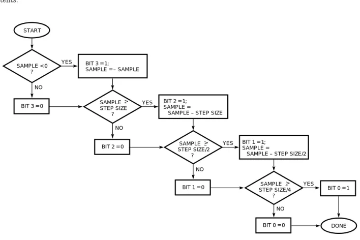
Figure 3 shows a block diagram of the quantization process used by the IMA algorithm. The quantizer outputs four bits representing the signed magnitude of the number of quantizer levels for each input sam-ple.
Adaptation to the audio signal takes place only in the quantizer block. The quantizer adapts the step size based on the current step size and the quan-tizer output of the immediately previous input. This adaptation can be done as a sequence of two table lookups. The three bits representing the number of quantizer levels serve as an index into the first table lookup whose output is an index adjustment for the second table lookup. This adjustment is added to a stored index value, and the range-limited result is used as the index to the second table lookup. The summed index value is stored for use in the next iteration of the step-size adaptation. The output of the second table lookup is the new quantizer step size. Note that given a starting value for the in-dex into the second table lookup, the data used for adaptation is completely deducible from the quan-tizer outputs; side information is not required for the quantizer adaptation. Figure 4 illustrates a block diagram of the step-size adaptation process, and Tables 1 and 2 provide the table lookup con-tents.
Table 1
First Table Lookup for the IMA ADPCM Quantizer Adaptation
Three Bits Quantized
Magnitude Index Adjustment
000 -1 001 -1 010 -1 011 -1 100 2 101 4 110 6 111 8 BIT 3 = 1; SAMPLE = – SAMPLE START SAMPLE < 0 ? > – YES NO
BIT 3 = 0 BIT 2 = 1;SAMPLE =
SAMPLE – STEP SIZE SAMPLE
STEP SIZE ?
YES
NO
BIT 2 = 0 BIT 1 = 1;SAMPLE =
SAMPLE – STEP SIZE/2 YES NO BIT 1 = 0 YES NO BIT 0 = 1 > – SAMPLE STEP SIZE/2 ? > – SAMPLE STEP SIZE/4 ? BIT 0 = 0 DONE
FIRST TABLE LOOKUP
DELAY FOR NEXT ITERATION OF STEP-SIZE ADAPTATION + + + LIMIT VALUE BETWEEN 0 AND 88 SECOND TABLE LOOKUP LOWER THREE BITS OF QUANTIZER OUTPUT INDEX ADJUSTMENT STEP SIZE
Figure 4 IMA ADPCM Step-size Adaptation
Table 2
Second Table Lookup for the IMA ADPCM Quantizer Adaptation
Index Step Size Index Step Size Index Step Size Index Step Size
0 7 22 60 44 494 66 4,026 1 8 23 66 45 544 67 4,428 2 9 24 73 46 598 68 4,871 3 10 25 80 47 658 69 5,358 4 11 26 88 48 724 70 5,894 5 12 27 97 49 796 71 6,484 6 13 28 107 50 876 72 7,132 7 14 29 118 51 963 73 7,845 8 16 30 130 52 1,060 74 8,630 9 17 31 143 53 1,166 75 9,493 10 19 32 157 54 1,282 76 10,442 11 21 33 173 55 1,411 77 11,487 12 23 34 190 56 1,552 78 12,635 13 25 35 209 57 1,707 79 13,899 14 28 36 230 58 1,878 80 15,289 15 31 37 253 59 2,066 81 16,818 16 34 38 279 60 2,272 82 18,500 17 37 39 307 61 2,499 83 20,350 18 41 40 337 62 2,749 84 22,358 19 45 41 371 63 3,024 85 24,623 20 50 42 408 64 3,327 86 27,086 21 55 43 449 65 3,660 87 29,794 88 32,767
IMA ADPCM: Error Recovery. A fortunate side effect of the design of this ADPCM scheme is that decoder errors caused by isolated code word errors or edits, splices, or random access of the compressed bit stream generally do not have a disastrous impact on decoder output. This is usually not true for com-pression schemes that use prediction. Since predic-tion relies on the correct decoding of previous audio samples, errors in the decoder tend to propagate. The next section explains why the error propagation is generally limited and not disastrous for the IMA algorithm. The decoder reconstructs the audio sam-ple, Xp[n], by adding the previously decoded audio sample, Xp[n—1]to the result of a signed magnitude product of the code word, C[n], and the quantizer step size plus an offset of one-half step size:
Xp[n] = Xp[n—1] + step_size[n]2C’ [n]
where C’ [n] = one-half plus a suitable numeric con-version of C [n].
An analysis of the second step-size table lookup reveals that each successive entry is about 1.1 times the previous entry. As long as range limiting of the second table index does not take place, the value for step_size[n] is approximately the product of the previous value, step_size[n—1], and a function of the code word, F(C[n—1]):
step_size[n]= step_size[n—1]2F(C[n—1]) The above two equations can be manipulated to express the decoded audio sample, Xp[n], as a func-tion of the step size and the decoded sample value at time, m, and the set of code words between time, m, and n Xp[n] = Xp[m]+step_size[m] 2 Pn i=m+1 f Qi j=m+1 F (C[j])g2C0[i]
Note that the terms in the summation are only a function of the code words from time m+1 onward. An error in the code word, C[q], or a random access entry into the bit stream at time q can result in an error in the decoded output, Xp[q], and the quan-tizer step size, step_size[q+1]. The above equation shows that an error in Xp[m] amounts to a constant offset to future values of Xp[n]. This offset is in-audible unless the decoded output exceeds its per-missible range and is clipped. Clipping results in a momentary audible distortion but also serves to correct partially or fully the offset term. Further-more, digital high-pass filtering of the decoder out-put can remove this constant offset term. The above equation also shows that an error in step_size[m+1] amounts to an unwanted gain or attenuation of fu-ture values of the decoded output Xp[n]. The shape
of the output wave form is unchanged unless the index to the second step-size table lookup is range limited. Range limiting results in a partial or full correction to the value of the step size.
The nature of the step-size adaptation limits the impact of an error in the step size. Note that an er-ror in step_size[m+1] caused by an erer-ror in a single code word can be at most a change of (1.1)9, or 7.45 dB in the value of the step size. Note also that any sequence of 88 code words that all have magnitude 3 or less (refer to Table 1) completely corrects the step size to its minimum value. Even at the lowest audio sampling rate typically used, 8 kHz, 88 sam-ples correspond to 11 milliseconds of audio. Thus random access entry or edit points exist whenever 11 milliseconds of low-level signal occur in the audio stream.
MPEG/Audio Compression
The Motion Picture Experts Group (MPEG) audio compression algorithm is an International Organi-zation for StandardiOrgani-zation (ISO) standard for high-fidelity audio compression. It is one part of a three-part compression standard. With the other two parts, video and systems, the composite standard addresses the compression of synchronized video and audio at a total bit rate of roughly 1.5 megabits per second.
Like -law and ADPCM, the MPEG/audio com-pression is lossy; however, the MPEG algorithm can achieve transparent, perceptually lossless compres-sion. The MPEG/audio committee conducted exten-sive subjective listening tests during the develop-ment of the standard. The tests showed that even with a 6-to-1 compression ratio (stereo, 16-bit-per-sample audio 16-bit-per-sampled at 48 kHz compressed to 256 kilobits per second) and under optimal listening con-ditions, expert listeners were unable to distinguish between coded and original audio clips with statisti-cal significance. Furthermore, these clips were spe-cially chosen because they are difficult to compress. Grewin and Ryden give the details of the setup, pro-cedures, and results of these tests.[9]
The high performance of this compression algo-rithm is due to the exploitation of auditory mask-ing. This masking is a perceptual weakness of the ear that occurs whenever the presence of a strong audio signal makes a spectral neighborhood of weaker audio signals imperceptible. This noise-masking phenomenon has been observed and cor-roborated through a variety of psychoacoustic ex-periments.[10]
Empirical results also show that the ear has a lim-ited frequency selectivity that varies in acuity from less than 100 Hz for the lowest audible frequencies to more than 4 kHz for the highest. Thus the audi-ble spectrum can be partitioned into critical bands that reflect the resolving power of the ear as a func-tion of frequency. Table 3 gives a listing of critical bandwidths.
Because of the ear’s limited frequency resolving power, the threshold for noise masking at any given frequency is solely dependent on the signal activity within a critical band of that frequency. Figure 5 il-lustrates this property. For audio compression, this property can be capitalized by transforming the au-dio signal into the frequency domain, then dividing the resulting spectrum into subbands that approx-imate critical bands, and finally quantizing each subband according to the audibility of quantization noise within that band. For optimal compression, each band should be quantized with no more lev-els than necessary to make the quantization noise inaudible. The following sections present a more detailed description of the MPEG/audio algorithm. MPEG/Audio Encoding and Decoding
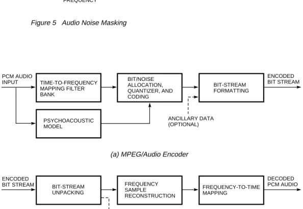
Figure 6 shows block diagrams of the MPEG/audio encoder and decoder.[11,12] In this high-level rep-resentation, encoding closely parallels the process described above. The input audio stream passes through a filter bank that divides the input into multiple subbands. The input audio stream simul-taneously passes through a psychoacoustic model that determines the signal-to-mask ratio of each subband. The bit or noise allocation block uses the signal-to-mask ratios to decide how to apportion the total number of code bits available for the quanti-zation of the subband signals to minimize the au-dibility of the quantization noise. Finally, the last block takes the representation of the quantized au-dio samples and formats the data into a decodable bit stream. The decoder simply reverses the for-matting, then reconstructs the quantized subband values, and finally transforms the set of subband values into a time-domain audio signal. As speci-fied by the MPEG requirements, ancillary data not necessarily related to the audio stream can be fitted within the coded bit stream.
The MPEG/audio standard has three distinct lay-ers for compression. Layer I forms the most basic algorithm, and Layers II and III are enhancements that use some elements found in Layer I. Each suc-cessive layer improves the compression performance but at the cost of greater encoder and decoder com-plexity.
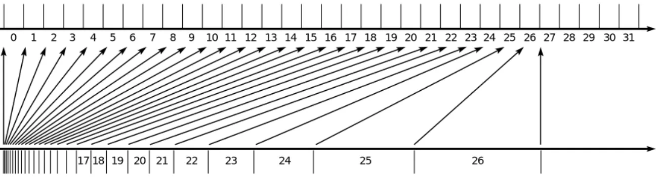
Layer I. The Layer I algorithm uses the basic filter bank found in all layers. This filter bank divides the audio signal into 32 constant-width frequency bands. The filters are relatively simple and pro-vide good time resolution with reasonable frequency resolution relative to the perceptual properties of the human ear. The design is a compromise with three notable concessions. First, the 32 constant-width bands do not accurately reflect the ear’s crit-ical bands. Figure 7 illustrates this discrepancy. The bandwidth is too wide for the lower frequencies so the number of quantizer bits cannot be specifi-cally tuned for the noise sensitivity within each crit-ical band. Instead, the included critcrit-ical band with the greatest noise sensitivity dictates the number of quantization bits required for the entire filter band. Second, the filter bank and its inverse are not loss-less transformations. Even without quantization, the inverse transformation would not perfectly re-cover the original input signal. Fortunately, the er-ror introduced by the filter bank is small and inaudi-ble. Finally, adjacent filter bands have a significant frequency overlap. A signal at a single frequency can affect two adjacent filter bank outputs.
Table 3
Approximate Critical Band Boundaries
Band Number Frequency (Hz)1 Band Number Frequency (Hz)1 0 50 14 1,970 1 95 15 2,340 2 140 16 2,720 3 235 17 3,280 4 330 18 3,840 5 420 19 4,690 6 560 20 5,440 7 660 21 6,375 8 800 22 7,690 9 940 23 9,375 10 1,125 24 11,625 11 1,265 25 15,375 12 1,500 26 20,250 13 1,735
,,,
,,,,,,,,,,
STRONG TONAL SIGNAL
REGION WHERE WEAKER SIGNALS ARE MASKED
FREQUENCY
AMPLITUDE
Figure 5 Audio Noise Masking
TIME-TO-FREQUENCY MAPPING FILTER BANK PSYCHOACOUSTIC MODEL PCM AUDIO INPUT ENCODED BIT STREAM BIT/NOISE ALLOCATION, QUANTIZER, AND CODING BIT-STREAM FORMATTING ANCILLARY DATA (OPTIONAL)
(a) MPEG/Audio Encoder
BIT-STREAM UNPACKING ENCODED BIT STREAM DECODED PCM AUDIO FREQUENCY SAMPLE RECONSTRUCTION FREQUENCY-TO-TIME MAPPING ANCILLARY DATA (IF ENCODED) (b) MPEG/Audio Decoder
31 30 29 28 27 26 25 24 23 22 21 20 19 18 17 16 15 14 13 12 11 10 9 8 7 6 5 4 3 2 1 0 26 25 24 23 22 21 20 19 18 17
MPEG/AUDIO FILTER BANK BANDS
CRITICAL BAND BOUNDARIES
Figure 7 MPEG/Audio Filter Bandwidths versus Critical Bandwidths The filter bank provides 32 frequency samples, one
sample per band, for every 32 input audio samples. The Layer I algorithm groups together 12 samples from each of the 32 bands. Each group of 12 sam-ples receives a bit allocation and, if the bit alloca-tion is not zero, a scale factor. Coding for stereo redundancy compression is slightly different and is discussed later in this paper. The bit allocation de-termines the number of bits used to represent each sample. The scale factor is a multiplier that sizes the samples to maximize the resolution of the quan-tizer. The Layer I encoder formats the 32 groups of 12 samples (i.e., 384 samples) into a frame. Besides the audio data, each frame contains a header, an optional cyclic redundancy code (CRC) check word, and possibly ancillary data.
Layer II. The Layer II algorithm is a simple en-hancement of Layer I. It improves compression per-formance by coding data in larger groups. The Layer II encoder forms frames of 3 by 12 by 32 = 1,152 samples per audio channel. Whereas Layer I codes data in single groups of 12 samples for each sub-band, Layer II codes data in 3 groups of 12 samples for each subband. Again discounting stereo redun-dancy coding, there is one bit allocation and up to three scale factors for each trio of 12 samples. The encoder encodes with a unique scale factor for each group of 12 samples only if necessary to avoid audi-ble distortion. The encoder shares scale factor val-ues between two or all three groups in two other cases: (1) when the values of the scale factors are sufficiently close and (2) when the encoder antici-pates that temporal noise masking by the ear will hide the consequent distortion. The Layer II algo-rithm also improves performance over Layer I by representing the bit allocation, the scale factor val-ues, and the quantized samples with a more efficient code.
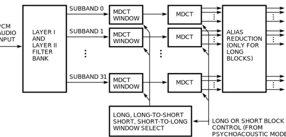
Layer III. The Layer III algorithm is a much more refined approach.[13,14] Although based on the same filter bank found in Layers I and II, Layer III compensates for some filter bank deficiencies by processing the filter outputs with a modified discrete cosine transform (MDCT). Figure 8 shows a block diagram of the process.
The MDCTs further subdivide the filter bank out-puts in frequency to provide better spectral resolu-tion. Because of the inevitable trade-off between time and frequency resolution, Layer III specifies two different MDCT block lengths: a long block of 36 samples or a short block of 12. The short block length improves the time resolution to cope with transients. Note that the short block length is one-third that of a long block; when used, three short blocks replace a single long block. The switch be-tween long and short blocks is not instantaneous. A long block with a specialized long-to-short or short-to-long data window provides the transition mech-anism from a long to a short block. Layer III has three blocking modes: two modes where the outputs of the 32 filter banks can all pass through MDCTs with the same block length and a mixed block mode where the 2 lower-frequency bands use long blocks and the 30 upper bands use short blocks.
LAYER I AND LAYER II FILTER BANK ALIAS REDUCTION (ONLY FOR LONG BLOCKS) PCM AUDIO INPUT SUBBAND 0 MDCT WINDOW SUBBAND 1 MDCT WINDOW SUBBAND 31 MDCT WINDOW MDCT MDCT MDCT LONG, LONG-TO-SHORT SHORT, SHORT-TO-LONG WINDOW SELECT
LONG OR SHORT BLOCK CONTROL (FROM PSYCHOACOUSTIC MODEL)
Figure 8 MPEG/Audio Layer III Filter Bank Processing, Encoder Side Other major enhancements over the Layer I and
Layer II algorithms include:
• Alias reduction — Layer III specifies a method of processing the MDCT values to remove some redundancy caused by the overlapping bands of the Layer I and Layer II filter bank.
• Nonuniform quantization — The Layer III tizer raises its input to the 3/4 power before quan-tization to provide a more consistent signal-to-noise ratio over the range of quantizer values. The requantizer in the MPEG/audio decoder re-linearizes the values by raising its output to the 4/3 power.
• Entropy coding of data values — Layer III uses Huffman codes to encode the quantized samples for better data compression.[15]
• Use of a bit reservoir — The design of the Layer III bit stream better fits the variable length na-ture of the compressed data. As with Layer II, Layer III processes the audio data in frames of 1,152 samples. Unlike Layer II, the coded data representing these samples does not necessar-ily fit into a fixed-length frame in the code bit stream. The encoder can donate bits to or bor-row bits from the reservoir when appropriate. • Noise allocation instead of bit allocation — The
bit allocation process used by Layers I and II only approximates the amount of noise caused by quantization to a given number of bits. The Layer III encoder uses a noise allocation iteration loop. In this loop, the quantizers are varied in an orderly way, and the resulting quantization noise
is actually calculated and specifically allocated to each subband.
The Psychoacoustic Model
The psychoacoustic model is the key component of the MPEG encoder that enables its high perfor-mance.[16,17,18,19] The job of the psychoacoustic model is to analyze the input audio signal and de-termine where in the spectrum quantization noise will be masked and to what extent. The encoder uses this information to decide how best to repre-sent the input audio signal with its limited number of code bits. The MPEG/audio standard provides two example implementations of the psychoacoustic model. Below is a general outline of the basic steps involved in the psychoacoustic calculations for ei-ther model.
• Time align audio data — The psychoacoustic model must account for both the delay of the au-dio data through the filter bank and a data off-set so that the relevant data is centered within its analysis window. For example, when using psychoacoustic model two for Layer I, the de-lay through the filter bank is 256 samples, and the offset required to center the 384 samples of a Layer I frame in the 512-point psychoacoustic analysis window is (512 — 384)/2 = 64 points. The net offset is 320 points to time align the psy-choacoustic model data with the filter bank out-puts.
• Convert audio to spectral domain — The psy-choacoustic model uses a time-to-frequency map-ping such as a 512- or 1,024-point Fourier
trans-form. A standard Hann weighting, applied to audio data before Fourier transformation, condi-tions the data to reduce the edge effects of the transform window. The model uses this sepa-rate and independent mapping instead of the fil-ter bank outputs because it needs finer frequency resolution to calculate the masking thresholds. • Partition spectral values into critical bands —
To simplify the psychoacoustic calculations, the model groups the frequency values into percep-tual quanta.
• Incorporate threshold in quiet — The model in-cludes an empirically determined absolute mask-ing threshold. This threshold is the lower bound for noise masking and is determined in the ab-sence of masking signals.
• Separate into tonal and nontonal components — The model must identify and separate the tonal and noiselike components of the audio signal be-cause the noise-masking characteristics of the two types of signal are different.
• Apply spreading function — The model deter-mines the noise-masking thresholds by applying an empirically determined masking or spreading function to the signal components.
• Find the minimum masking threshold for each subband — The psychoacoustic model calculates the masking thresholds with a higher-frequency resolution than provided by the filter banks. Where the filter band is wide relative to the crit-ical band (at the lower end of the spectrum), the model selects the minimum of the masking thresholds covered by the filter band. Where the filter band is narrow relative to the critical band, the model uses the average of the masking thresholds covered by the filter band.
• Calculate signal-to-mask ratio — The psychoa-coustic model takes the minimum masking thresh-old and computes the signal-to-mask ratio; it then passes this value to the bit (or noise) al-location section of the encoder.
Stereo Redundancy Coding
The MPEG/audio compression algorithm supports two types of stereo redundancy coding: intensity stereo coding and middle/side (MS) stereo coding. Both forms of redundancy coding exploit another perceptual weakness of the ear. Psychoacoustic re-sults show that, within the critical bands cover-ing frequencies above approximately 2 kHz, the ear bases its perception of stereo imaging more on the temporal envelope of the audio signal than its tem-poral fine structure. All layers support intensity stereo coding. Layer III also supports MS stereo coding.
In intensity stereo mode, the encoder codes some upper-frequency filter bank outputs with a single summed signal rather than send independent codes for left and right channels for each of the 32 fil-ter bank outputs. The intensity sfil-tereo decoder re-constructs the left and right channels based only on independent left- and right-channel scale factors. With intensity stereo coding, the spectral shape of the left and right channels is the same within each intensity-coded filter bank signal, but the magni-tude is different.
The MS stereo mode encodes the signals for left and right channels in certain frequency ranges as middle (sum of left and right) and side (difference of left and right) channels. In this mode, the encoder uses specially tuned techniques to further compress side-channel signal.
Real-time Software Implementations
The software-only implementations of the-law and ADPCM algorithms can easily run in real time. A single table lookup can do-law compression or decompression. A software-only implementation of the IMA ADPCM algorithm can process stereo, 44.1-kHz-sampled audio in real time on a 20-MHz 386-class computer. The challenge lies in developing a real-time software implementation of the MPEG/ audio algorithm. The MPEG standards document does not offer many clues in this respect. There are much more efficient ways to compute the calcu-lations required by the encoding and decoding pro-cesses than the procedures outlined by the standard. As an example, the following section details how the number of multiplies and additions used in a certain calculation can be reduced by a factor of 12.Figure 9 shows a flow chart for the analysis sub-band filter used by the MPEG/audio encoder. Most of the computational load is due to the second-from-last block. This block contains the following matrix multiply: S(i) = 63 X k=0 Y (k)2cos (22i + 1)2(k 0 16)2II 64 fori =0 ... 31.
Using the above equation, each of the 31 values of S(i) requires 63 adds and 64 multiplies. To optimize this calculation, note that the M(i,k) coefficients are similar to the coefficients used by a 32-point, un-normalized inverse discrete cosine transform (DCT) given by f(i) = 31 X k=0 F (k)2cos (22i + 1)2k2II 64 fori =0 ... 31.
Indeed, S(i) is identical to f(i) if F(k) is computed as follows = for F(k) Y (16) k= 0; =Y (k + 16)+Y (16 − k) k= 1 ... 16; =Y (k + 16)+Y (80 − k) k= 17 ... 31. for for
Thus with the almost negligible overhead of comput-ing the F(k) values, a twofold reduction in multiplies and additions comes from halving the range that k varies. Another reduction in multiplies and addi-tions of more than sixfold comes from using one of many possible fast algorithms for the computation of the inverse DCT.[20,21,22] There is a similar opti-mization applicable to the 64 by 32 matrix multiply found within the decoder’s subband filter bank.
Many other optimizations are possible for both MPEG/audio encoder and decoder. Such optimiza-tions enable a software-only version of the MPEG /audio Layer I or Layer II decoder (written in the C programming language) to obtain real-time perfor-mance for the decoding of high-fidelity monophonic audio data on a DECstation 5000 Model 200. This workstation uses a 25-MHz R3000 MIPS CPU and has 128 kilobytes of external instruction and data cache. With this optimized software, the MPEG /audio Layer II algorithm requires an average of 13.7 seconds of CPU time (12.8 seconds of user time and 0.9 seconds of system time) to decode 7.47 sec-onds of a stereo audio signal sampled at 48 kHz with 16 bits per sample.
Although real-time MPEG/audio decoding of stereo audio is not possible on the DECstation 5000, such decoding is possible on Digital’s workstations equipped with the 150-MHz DECchip 21064 CPU (Alpha AXP architecture) and 512 kilobytes of exter-nal instruction and data cache. Indeed, when this same code (i.e., without CPU-specific optimization) is compiled and run on a DEC 3000 AXP Model 500 workstation, the MPEG/audio Layer II algorithm re-quires an average of 4.2 seconds (3.9 seconds of user time and 0.3 seconds of system time) to decode the same 7.47-second audio sequence.
SHIFT IN 32 NEW SAMPLES INTO 512-POINT FIFO BUFFER, Xi
WINDOW SAMPLES: FOR i = 0 TO 511, DO Zi = Ci Xi PARTIAL CALCULATION: FOR i = 0 TO 63, DO CALCULATE 32 SAMPLES BY MATRIXING Yi Mi,k 63 k = 0 Si =
OUTPUT 32 SUBBAND SAMPLES Zi + 64 j 7 j = 0
Yi =
Figure 9 Flow Diagram of the MPEG/Audio Encoder Filter Bank
Summary
Techniques to compress general digital audio sig-nals include -law and adaptive differential pulse code modulation. These simple approaches apply low-complexity, low-compression, and medium au-dio quality algorithms to auau-dio signals. A third technique, the MPEG/audio compression algorithm, is an ISO standard for high-fidelity audio compres-sion. The MPEG/audio standard has three layers of successive complexity for improved compression performance.
References
1. A. Oppenheim and R. Schafer, Discrete Time Sig-nal Processing (Englewood Cliffs, NJ: Prentice-Hall, 1989): 80-87.
2. K. Pohlman, Principles of Digital Audio (Indi-anapolis, IN: Howard W. Sams and Co., 1989). 3. J. Flanagan, Speech Analysis Synthesis and
Per-ception (New York: Springer-Verlag, 1972).
4. B. Atal, "Predictive Coding of Speech at Low Rates," IEEE Transactions on Communications, vol. COM-30, no. 4 (April 1982).
5. CCITT Recommendation G.711: Pulse Code Mod-ulation (PCM) of Voice Frequencies (Geneva: In-ternational Telecommunications Union, 1972). 6. L. Rabiner and R. Schafer, Digital Processing of
Speech Signals (Englewood Cliffs, NJ: Prentice-Hall, 1978).
7. M. Nishiguchi, K. Akagiri, and T. Suzuki, "A New Audio Bit Rate Reduction System for the CD-I Format," Preprint 2375, 81st Audio Engineering Society Convention, Los Angeles (1986).
8. Y. Takahashi, H. Yazawa, K. Yamamoto, and T. Anazawa, "Study and Evaluation of a New Method of ADPCM Encoding," Preprint 2813, 86th Audio Engineering Society Convention, Ham-burg (1989).
9. C. Grewin and T. Ryden, "Subjective Assess-ments on Low Bit-rate Audio Codecs," Proceed-ings of the Tenth International Audio Engineer-ing Society Conference, London (1991):91-102.
10.J. Tobias, Foundations of Modern Auditory The-ory (New York and London: Academic Press, 1970): 159-202.
11.K. Brandenburg and G. Stoll, "The ISO/MPEG-Audio Codec: A Generic Standard for Coding of High Quality Digital Audio," Preprint 3336, 92nd Audio Engineering Society Convention, Vienna (1992).
12.K. Brandenburg and J. Herre, "Digital Au-dio Compression for Professional Applications," Preprint 3330, 92nd Audio Engineering Society Convention, Vienna (1992).
13.K. Brandenburg and J. D. Johnston, "Second Generation Perceptual Audio Coding: The Hy-brid Coder," Preprint 2937, 88th Audio Engineer-ing Society Convention, Montreaux (1990). 14.K. Brandenburg, J. Herre, J. D. Johnston, Y.
Mahieux, and E. Schroeder, "ASPEC: Adap-tive Spectral Perceptual Entropy Coding of High Quality Music Signals," Preprint 3011, 90th Au-dio Engineering Society Convention, Paris (1991). 15.D. Huffman, "A Method for the Construction of Minimum Redundancy Codes," Proceedings of the IRE, vol. 40 (1962) : 1098-1101.
16.J. D. Johnston, "Estimation of Perceptual En-tropy Using Noise Masking Criteria," Proceed-ings of the 1988 IEEE International Confer-ence on Acoustics, Speech, and Signal Processing (1988) : 2524-2527.
17.J. D. Johnston, "Transform Coding of Audio Signals Using Perceptual Noise Criteria," IEEE Journal on Selected Areas in Communications, vol. 6 (February 1988): 314-323.
18.K. Brandenburg, "OCF — A New Coding Algo-rithm for High Quality Sound Signals," Proceed-ings of the 1987 IEEE ICASSP (1987): 141-144. 19.D. Wiese and G. Stoll, "Bitrate Reduction of High
Quality Audio Signals by Modeling the Ear’s Masking Thresholds," Preprint 2970, 89th Au-dio Engineering Society Convention, Los Angeles (1990).
20.J. Ward and B. Stanier, "Fast Discrete Cosine Transform Algorithm for Systolic Arrays," Elec-tronics Letters, vol. 19, no. 2 (January 1983). 21.J. Makhoul, "A Fast Cosine Transform in One
and Two Dimensions," IEEE Transactions on Acoustics, Speech, and Signal Processing, vol. ASSP-28, no. 1 (February 1980).
22.W.-H. Chen, C. H. Smith, and S. Fralick, "A Fast Computational Algorithm for the Discrete Cosine Transform," IEEE Transactions on Communica-tions, vol. COM-25, no. 9 (September 1977).
Trademarks
The following are trademarks of Digital Equip-ment Corporation: Digital, DECstation, DEC 3000 AXP, and DECchip 21064.
MIPS is a trademark of MIPS Computer Systems, Inc.
Biography
Davis Yen Pan Davis Pan joined Digital in 1986
after receiving a Ph.D. in electrical engineering from MIT. A principal engineer in the Alpha Personal Systems Group, he is responsible for the develop-ment of audio signal processing algorithms for mul-timedia products. He was project leader for the Alpha/OSF base audio driver. He is a participant in the Interactive Multimedia Association Digital Audio Technical Working Group, the ANSI X3L3.1 Technical Working Group on MPEG standards ac-tivities, and the ISO/MPEG standards committee. Davis is also chair of the ISO/MPEG ad hoc com-mittee of MPEG/audio software verification.