Narrowest-over-threshold detection of multiple change-points and
change-point-like features
LSE Research Online URL for this paper:
http://eprints.lse.ac.uk/100430/
Version: Published Version
Article:
Baranowski, Rafal, Chen, Yining and Fryzlewicz, Piotr (2019)
Narrowest-over-threshold detection of multiple change-points and change-point-like features.
Journal of the Royal Statistical Society. Series B: Statistical Methodology, 81 (3).
pp. 649-672. ISSN 1369-7412
https://doi.org/10.1111/rssb.12322
[email protected]
https://eprints.lse.ac.uk/
Reuse
This article is distributed under the terms of the Creative Commons Attribution (CC BY) licence. This licence allows you to distribute, remix, tweak, and build upon the work, even commercially, as long as you credit the authors for the original work. More information and the full terms of the licence here: https://creativecommons.org/licenses/
2019 The Authors Journal of the Royal Statistical Society: Series B
(Statistical Methodology) Published by John Wiley & Sons Ltd on behalf of the Royal Statistical Society.
This is an open access article under the terms of the Creative Commons Attribution License, which permits use, distribution and reproduction in any medium, provided the original work is properly cited.
1369–7412/19/81649
81,Part3,pp.649–672
Narrowest-over-threshold detection of multiple
change points and change-point-like features
Rafal Baranowski, Yining Chen and Piotr FryzlewiczLondon School of Economics and Political Science, UK [Received January 2017. Final revision April 2019]
Summary. We propose a new, generic and flexible methodology for non-parametric function estimation, in which we first estimate the number and locations of any features that may be present in the function and then estimate the function parametrically between each pair of neighbouring detected features. Examples of features handled by our methodology include change points in the piecewise constant signal model, kinks in the piecewise linear signal model and other similar irregularities, which we also refer to as generalized change points. Our methodology works with only minor modifications across a range of generalized change point scenarios, and we achieve such a high degree of generality by proposing and using a new multiple generalized change point detection device, termed narrowest-over-threshold (NOT) detection. The key ingredient of the NOT method is its focus on the smallest local sections of the data on which the existence of a feature is suspected. For selected scenarios, we show the consistency and near optimality of the NOT algorithm in detecting the number and locations of generalized change points. The NOT estimators are easy to implement and rapid to compute. Importantly, the NOT approach is easy to extend by the user to tailor to their own needs. Our methodology is implemented in the R package not.
Keywords: Break point detection; Knots; Piecewise polynomial; Segmentation; Splines
1. Introduction
This paper considers the canonical univariate statistical model
Yt=ft+"t, t=1,: : :,T, .1/ where the deterministic and unknown signal ft is believed to display some regularity across the indext, and the stochastic noise"t is exactly or approximately centred at zero. Despite the simplicity of model (1), inferring information aboutftremains a task of fundamental importance in modern applied statistics and data science. When the interest is in the detection of ‘features’ inftsuch as jumps or kinks, then non-linear techniques are usually required.
Ifftis modelled as piecewise constant and it is of interest to detect its change points, several techniques are available, and we mention only a selection. For Gaussian noise"t, both non-penalized and non-penalized least squares approaches were considered by Yao and Au (1989). For specific choices of penalty functions, see for example Yao (1988), Lavielle (2005) and Davis
et al.(2006). The Gaussianity assumption on"twas relaxed to exponential family distributions in Lee (1997), Hawkins (2001) and Fricket al.(2014). In particular, Frick et al.(2014) also provided confidence intervals for the location of the estimated change points. Often this penalty-type approach requires a computational cost of at leastO.T2/. However, there are exceptions, Address for correspondence: Yining Chen, Department of Statistics, London School of Economics and Political Science, Columbia House, Houghton Street, London, WC2A 2AE, UK.
such as the pruned exact linear time (PELT) method (Killick, Fearnhead and Eckley, 2012), which achieves a linear computational cost, but requires the further assumption that change points are separated by time intervals drawn independently from some probability distribution: a scenario in which considerations of statistical consistency are not generally possible. A non-parametric version of the PELT method was investigated by Haynes et al.(2017). Another general approach is based on the idea of binary segmentation (BS) (Vostrikova, 1981), which can be viewed as a greedy approach with a limited computational cost. Its popular variants include circular binary segmentation (CBS) (Olshenet al., 2004) and wild binary segmentation (WBS) (Fryzlewicz, 2014). A selection of publications and software can be found in the on-line repositorychangepoint.infomaintained by Killick, Nam, Aston and Eckley (2012).
More general change point problems, in whichft is modelled as piecewise parametric (not necessarily piecewise constant) between ‘knots’, the number and locations of which are unknown and need to be estimated, have attracted less interest in the literature and overwhelmingly focus on linear trend detection. Among them, we mention the approach based on the least squares principle and Wald-type tests by Bai and Perron (1998), dynamic programming using theL0 -penalty (Maidstoneet al., 2017) and trend filtering (Tibshirani, 2014; Linet al., 2017). Finally, we mention a related problem of jump regression, where the aim is to estimate the points of sharp cusps or discontinuities of a regression function. As investigated in, for example, Wang (1995) and Xia and Qiu (2015), it proceeds by estimating the locations of features non-parametrically via wavelets or local kernel smoothing.
The aim of this work is to propose a new generic approach to the problem of detecting an unknown number of ‘features’ occurring at unknown locations inft. By a feature, we mean a characteristic offt, occurring at a locationt0, that is detectable by considering a sufficiently large subsample of dataYtaroundt0. Examples include change points inftwhen it is modelled as piecewise constant, change points in the first derivative whenft is modelled as piecewise linear and continuous, and discontinuities inft or its first derivative whenft is modelled as piecewise linear but without the continuity constraint. We shall provide a precise description of the type of features that we are interested in later. Moving beyondftonly, our approach will also permit the detection of similar features in some distributional aspects of"t, e.g. in its variance. Since all types of features that we consider describe changes in a parametric description offt, we use the terms ‘feature detection’ and ‘change point detection’ interchangeably throughout the paper. Occasionally, for precision, we shall be referring to change point detection in the piecewise constant model as the ‘canonical’ change point problem, whereas our general feature detection problem will sometimes be referred to as a ‘generalized’ change point problem.
Core to our approach is a particular blend of ‘global’ and ‘local’ treatment of the dataYtin the search for the multiple features that may be present inft: a combination that gives our method a multiscale character. At the first global stage, we randomly draw a number of subsamples .Ys+1,: : :,Ye/′, where 0s < eT. On each subsample, we assume, possibly erroneously, that
only one feature is present and use a tailor-made contrast function derived (according to a universal recipe that we provide later) from the likelihood theory to find the most likely location of the feature. We retain those subsamples for which the contrastexceeds a certain user-specified thresholdand discard the others. Among the subsamples retained, we search for the subsample that is drawn on thenarrowest interval, i.e. one for whiche−sis the smallest: it is this step that gives rise to the namenarrowest over threshold(NOT) for our methodology. The focus on the narrowest interval constitutes the local part of the method and is a key ingredient of our approach which ensures that, with high probability, at most one feature is present in the interval selected. This key observation gives our methodology a general character and enables it to be used, only with minor modifications, in a wide range of scenarios, including those described in
the previous paragraph. Having detected the first feature, the algorithm then proceeds recursively to the left and to the right of it, and stops, on any current interval, if no contrasts can be found that exceed the threshold.
Besides its generic character, other benefits of the methodology proposed include low compu-tational complexity, ease of implementation, accuracy in the detection of the feature locations and the fact that it enables parametric estimation of the signal on each section delimited by a pair of neighbouring estimated features. Regarding the computational complexity, the fact that typical contrasts are computable in linear time leads to a computational complexity of O.MT/for the entire procedure; typically, only a limited number of data subsamples,M, need to be drawn (we provide precise bounds later; with finitely many change points, we can take M=O{log.T/}in general). Moreover, the entire threshold-indexed solution path can also be computed efficiently, in typically close-to-linear time, as observed from our numerical experi-ments. Regarding the estimation accuracy, in the scenarios that we consider theoretically, our procedure yields nearly optimal rates of convergence for the estimators of feature locations.
On a broader level, our methodology promotes the idea of fitting simple models on subsets of the data (the local aspect), and then aggregating the results to obtain the overall fit (the global aspect): an idea that is also present in the WBS method of Fryzlewicz (2014). However, we emphasize that the way that the simple models (here: models containingat most onechange point or feature) are fitted in the NOT and WBS methods are entirely different and have different aims. Unlike WBS, the NOT methodology focuses on thenarrowestintervals of the data on which it is possible to locate the feature of interest. It is this focus that enables NOT detection to extend beyond change point detection for a piecewise constantft, the latter being the sole focus of the WBS method. The lack of the narrowest interval focus in the WBS and BS methods means that they are not applicable to more general feature detection, and we explain the mechanics of this important phenomenon briefly in the following simple example.
Consider a continuous piecewise linear signal that has two change points:
ft= ⎧ ⎪ ⎪ ⎪ ⎨ ⎪ ⎪ ⎪ ⎩ 1 350t, t=1,: : :, 350, 1, t=351,: : :, 650, 1001 350 − 1 350t, t=651,: : :, 1000. .2/
If we approximateftby using a piecewise linear signal with only one change point in its derivative, then the best approximation (in terms of minimizing thel2-distance) will result in an estimated change point att=500, which is away from the true change points att=350 andt=650, as is illustrated in Fig. 1. Therefore, taking the entire sample of data and searching for one of its multiple change points by fitting, via least squares, a triangular signal with a single change point does not make sense. It is this issue that leads to the failure of the BS and WBS methods for signals that are not piecewise constant. In contrast, NOT detection avoids this issue because of its unique feature of picking thenarrowest intervals, which are likely to contain only one change point. To understand the mechanics of this key feature, imagine that nowftis observed with noise. Through its pursuit of the narrowest intervals, NOT detection will ensure that, with high probability, some suitably narrow intervals around the change pointst=350 andt=650 are considered. More precisely, by construction, they will besufficiently narrow to contain only one change point each, but sufficiently wide for the designed contrast (see Section 2.3 for more on contrasts) to indicate the existence of the change point within both of them. The designed contrast function will indicate the correct location of the change point (modulothe estimation
(a) (b) (c)
Fig. 1. Bestl2-approximation ( ) of the true signal ( ) via a triangular signal with a single change point, the location of which is fixed at (a) the left change point, (b) halfway between the true change points and (c) at the right change point (approximation errors are given in terms of squaredl2-distance): (a)τD350, errorD15.0; (b)τD500, errorD6.3; (c)τD651, errorD15.0
error) if only one change point is present in the data subsample that is considered, unlike in the situation that was described earlier in which multiple change points were included in the chosen interval. More details on this example are presented in section C.3 of the on-line supplementary materials.
This example is different from the canonical change point detection problem (i.e. piecewise constant signal with multiple change points) where, if we approximate the signal by using a piecewise constant function with only one change point, the change point of the fitted signal will always be among the true change points (Venkatraman, 1992). Since the latter property does not hold in most generalized change point detection problems, this highlights the need for new methods with better localization of the feature of interest, such as our NOT algorithm. Fanget al.(2019) independently considered a related shortest interval idea in the context of the canonical change point detection problem. However, they did not consider it as a springboard to more general feature detection problems, which is the key motivation behind NOT detection and its most valuable contribution.
The remainder of this paper is organized as follows. In Section 2, we give a mathematical de-scription of the NOT algorithm. In particular, we consider the NOT approach in four scenarios, each with a different form of structural change in the mean and/or variance. For the development of both theory and computation, in selected scenarios, we introduce the tailor-made contrast function that is derived from the generalized likelihood ratio (GLR). Theoretical properties of the NOT algorithm, such as its consistency and convergence rates are also provided. In Section 3, we propose to use the NOT method with the strengthened Schwarz information criterion sSIC and discuss its computational aspects and theoretical properties. Section 4 discusses possible ex-tensions of the NOT method. A comprehensive simulation study is carried out in Section 5, where we compare NOT with the state of the art change point detection tools. In Section 6, we consider data examples of global temperature anomalies and London housing data. All proofs, together with details on the construction of the contrast functions, the computational aspects and exten-sion of the NOT method and further discusexten-sion on model misspecification, as well as additional simulations and a real data example, can be found in the on-line supplementary materials. 2. The narrowest-over-threshold framework
2.1. Set-up
To describe the main NOT framework, we consider a simplified version of model (1), where
Yt=ft+σt"t, t=1,: : :,T, .3/ whereftis the signal, and whereσtis the noise’s standard deviation at timet. To facilitate the technical presentation of our results, in Sections 2 and 3, we assume that"t∼IIDN.0, 1/. In Section 4, we extend our framework to other types of noise.
We assume that .ft,σt/can be partitioned into q+1 segments, with q unknown distinct change points 0=τ0<τ1< : : : <τq<τq+1=T. Here the value ofqis not prespecified and can grow withT. For eachj=1,: : :,q+1 and for t=τj−1+1,: : :,τj, the structure of .ft,σt/is modelled parametrically by a local (i.e. depending onj) real-valuedd-dimensional parameter vectorΘj(withΘj=Θj−1), wheredis known and typically small. To fix ideas, in what follows, we assume that each segment offt andσt follows a polynomial. In addition, we require the minimum distance between consecutive change points to be d or greater for the purpose of identifiability. (Otherwise, for example, takeft to be piecewise linear with a known constant
σt, in which cased=2; if we had a segment of length 1, then we would not be able to define a line based on a single point.) In other words,.ft,σt/can be divided intoqdifferent segments, each from the same parametric family of much simpler structure. Some commonly encountered scenarios are listed below, where the following assumptions hold inside thejth segment for each j=1,: : :,q+1.
(a) Constant variance, piecewise constant mean(scenario 1):σt=σ0andft=θjfort=τj−1+ 1,: : :,τj.
(b) Constant variance, continuous and piecewise linear mean (scenario 2):σt=σ0and ft= θj,1+θj,2tfort=τj−1+1,: : :,τj, with the additional constraint of
θj,1+θj,2τj=θj+1,1+θj+1,2τj forj=1,: : :,q.
(c) Constant variance, piecewise linear (but not necessarily continuous) mean (scenario 3):
σt=σ0 and ft=θj,1+θj,2t for t=τj−1+1,: : :,τj. In addition, fτj+θj,2=fτj+1 for j=1,: : :,q.
(d) Piecewise constant variance, piecewise constant mean(scenario 4):ft=θj,1andσt=θj,2>0 fort=τj−1+1,: : :,τj.
Sinceσ0 in scenarios 1–3 acts as a nuisance parameter, in the rest of this paper, for sim-plicity we assume that its value is known. If it is unknown, then it can be estimated accu-rately by using the median absolute deviation (MAD) method (Hampel, 1974). More specifi-cally, with independent and identically distributed (IID) Gaussian errors, the MAD estimator ofσ0is defined as ˆσ=median.|Y2−Y1|,: : :,|YT −YT−1|/={Φ−1.34/
√
2} in scenario 1, and as ˆ
σ=median.|Y1−2Y2+Y3|,: : :,|YT−2−2YT−1+YT|/={Φ−1.34/√6}in scenarios 2 and 3. Here
Φ−1.·/denotes the quantile function of the standard normal distribution. Note that the MAD estimator is robust to any change points in the underlying signalft, because of its combination of working with the differenced data, and its use of the median. Finally, we note that a different procedure is proposed to estimateσ0with dependent errors; see Section 4.1 for more details.
2.2. Main idea
We now describe the main idea of the NOT method formally; more details can be found in Section 2.4, where the pseudocode of the NOT algorithm is given.
In the first step, instead of directly using the entire data sample, we randomly extract subsam-ples, i.e. vectors.Ys+1,: : :,Ye/′, where.s,e/is drawn uniformly from the set of pairs of indices
in{0,: : :,T−1}×{1,: : :,T}that satisfy 0s < eT. Letl.Ys+1,: : :,Ye;Θ/be the likelihood ofΘgiven.Ys+1,: : :,Ye/′. We then compute the GLR statistic for all potential single change points within the subsample and pick the maximum, i.e.
Rb .s,e].Y/=2 log sup Θ1,Θ2{l.Ys+1,: : :,Yb;Θ1/l.Yb+1,: : :,Ye;Θ2/} supΘl.Ys+1,: : :,Ye;Θ/ ; R.s,e].Y/= max b∈{s+d,:::,e−d}R b .s,e].Y/: .4/
Here we also implicitly requiree−s2d, which comes from the identifiability condition, be-cause typically we need at leastdobservations to determineΘ1, and anotherdobservations to determineΘ2.
If constraints are in place betweenΘjandΘj+1for anyj=1,: : :,q(e.g. as in scenario 2), the supremum in the numerator of equation (4) is taken over the set that contains only elements of formΘ1×Θ2satisfying these constraints. Otherwise, as in scenarios 1, 3 and 4, equation (4) can be simplified to
Rb.s,e].Y/=2 log sup
Θl.Ys+1,: : :,Yb;Θ/supΘl.Yb+1,: : :,Ye;Θ/ supΘl.Ys+1,: : :,Ye;Θ/
: This procedure is repeated onMrandomly drawn pairs of integers.s1,e1/,: : :,.sM,eM/.
In the second step, we test allR.sm,em].Y/form=1,: : :,Magainst a given thresholdζT. Among those significantR.sm,em].Y/s, we pick the one corresponding to the interval.smÅ,emÅ] that has the smallest length. Once a change point has been found in.smÅ,emÅ] (i.e.bÅ that maximizes
Rb
.smÅ,emÅ].Y/: a function ofb), the same procedure is then repeated recursively to the left and to the right of it, until no further significant GLRs can be found. In each recursive step, we could reuse the previously drawn intervals, provided that they fall entirely within each current subsegment considered.
After the process of estimating the change points has been completed, we can estimate the signals within each segment by using standard methods such as least squares or maximum likelihood. Note that the estimation of knot locations in spline regression can be viewed as a multiple-change-point detection problem set in the context of polynomial segments that are continuously differentiable but have discontinuous higher order derivatives at the change points between these segments; NOT detection can be used for this purpose.
Admittedly, in our framework, one could also use a deterministic scheme (e.g. that in Ru-fibach and Walther (2010)) to pick a sufficiently rich family of intervals for multiscale inference. However, one advantage of our approach is that, through the use of randomness in drawing the intervals, we avoid having to make a subjective choice of a particular fixed design. Never-theless, with a very large number of intervals drawn, the difference in performance between the random and deterministic designs is likely to be minimal: an observation that was also made in Fryzlewicz (2014).
2.3. Log-likelihood ratios and contrast functions
In many applications, the GLR (4) in NOT detection can be simplified with the help of ‘contrast functions’ under the setting of Gaussian noise. In particular, these constructions mainly involve taking inner products between the data and other deterministic vectors, which greatly facilitates the development of both theory and computation, especially if these deterministic vectors are mutually orthonormal. In fact, the form of these contrast functions is crucial in our theoretical development.
More precisely, for every integer triple.s,e,b/with 0s < eT, our aim is to findCb .s,e].Y/ such that
(a) arg maxbCb.s,e].Y/=arg maxbRb.s,e].Y/, (b) heuristically speaking, the value ofCb
.s,e].Y/is relatively small if there is no change point in.s,e] and
(c) the formulation ofCb
.s,e].Y/mainly consists of taking inner products between the data and certain contrast vectors.
In what follows, we give the contrast functions corresponding to scenarios 1 and 2, where the aforementioned properties are satisfied. Their details under scenarios 3 and 4, as well as a com-prehesive discussion on the construction, can be found in section B of the on-line supplementary materials. We note that this approach recovers the cumulative sum statistic in scenario 1, which is popular in this canonical change point detection setting. One can view the resulting statistics as generalizations of cumulative sum statistics under other scenarios.
2.3.1. Scenario 1
Hereftis piecewise constant. For any integer triple.s,e,b/with 0s < eT ands < b < e, we define the contrast vectorψb.s,e]=.ψb.s,e].1/,: : :,ψb.s,e].T//′as
ψ.sb,e].t/= ⎧ ⎪ ⎪ ⎪ ⎨ ⎪ ⎪ ⎪ ⎩ e −b .e−s/.b−s/ , t=s+1,: : :,b, − b −s .e−s/.e−b/ , t=b+1,: : :,e, 0, otherwise: .5/
Also, ifb∈{s+1,: : :,e−1}, then we setψb
.s,e].t/=0 for allt. As an illustration, plots ofψb.s,e] with various.s,e,b/are shown in Fig. 2(a).
For any vectorv=.v1,: : :,vT/′, we define the contrast function as
C.sb,e].v/= |v,ψb.s,e]|: .6/
(a)
(b)
Fig. 2. Plots of (a)ψb.s,e]and (b)φ.sb,e]given by respectively equation (5) and equation (7) forsD0,eD1000 and several values ofb: ,bD125; ,bD500; ,bD750
2.3.2. Scenario 2
Hereftis piecewise linear and continuous. For any triple.s,e,b/with 0s < eT ands+1< b < e, consider the contrast vectorφb.s,e]=.φb.s,e].1/,: : :,φb.s,e].T//′with
φb.s,e].t/= ⎧ ⎪ ⎪ ⎨ ⎪ ⎪ ⎩ αb
.s,e]β.s,e]b [{3.b−s/+.e−b/−1}t−{b.e−s−1/+2.s+1/.b−s/}], t=s+1,: : :,b, −α b .s,e] βb .s,e] [{3.e−b/+.b−s/+1}t−{b.e−s−1/+2e.e−b+1/}], t=b+1,: : :,e, 0, otherwise, .7/ where αsb,e= 6 l.l2−1/{1+.e−b+1/.b−s/+.e−b/.b−s−1/} 1=2 , βbs,e= .e −b+1/.e−b/ .b−s−1/.b−s/ 1=2
andl=e−s. Ifb∈{s+2,: : :,e−1}, then we setφb.s,e].t/=0 for allt. We illustrate the structure ofφb.s,e]in Fig. 2(b). The contrast function is then defined as
C.sb,e].v/= |v,φb.s,e]|: .8/
2.4. The narrowest-over-threshold algorithm
Here we present the pseudocode of a generic version of the NOT algorithm. The main ingredient of the NOT procedure is a contrast functionCb
.s,e].·/, which is chosen by the user, depending on the assumed nature of change points in the data, e.g. as exemplified by our scenarios 1 and 2 above, and scenarios 3 and 4 in section B of the on-line supplementary materials. In addition, some tuning parameters are needed:ζT>0 is the threshold with respect to which the contrast should be tested, whereas Mis the number of the intervals that are drawn in the procedure. Guidance on the choice ofζT andMis given in Section 3. In particular, there we advocate an automatic choice ofζT by combining the NOT algorithm with an information-based criterion, thus making our procedure threshold free.
To sum up, the input includes the data vectorY, the set ofFTM that contains all randomly drawn subintervals for testing and the global variableSfor the set of estimated change points initialized withS= ∅. Then the NOT algorithm is started recursively with.s,e]=.0,T] and a givenζT. Here the entire set ofFTM that contains all random intervals is generated before we start running algorithm 1 (Table 1). In this way, we are better able to control the computational complexity of the entire procedure.
2.5. Theoretical properties of narrowest-over-threshold method
In this section, we analyse the theoretical behaviour of the NOT algorithm in scenarios 1 and 2. We use infill asymptotics, which are standard in the literature ona posteriori change point detection. An attractive feature of our methodology is that proofs for other scenarios can in principle be constructed ‘at home’ by the user, by following the same generic proof strategy as the strategy that we use for these two scenarios.
First, we revisit the canonical change point detection problem, scenario 1, where the signal vectorf=.f1,: : :,fT/′is piecewise constant. Hereσ0is assumed to be known. Otherwise, one
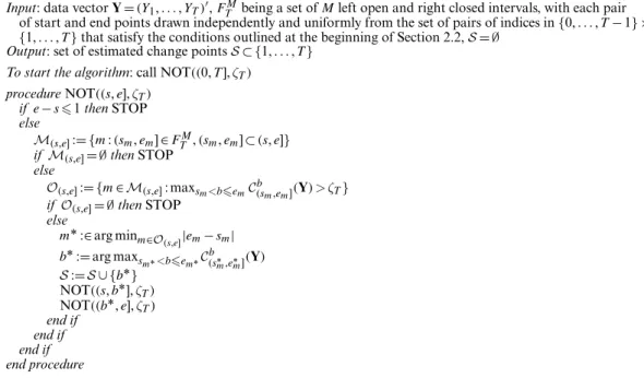
Table 1. Algorithm 1—NOT algorithm
Input: data vectorY=.Y1,: : :,YT/′,FTMbeing a set ofMleft open and right closed intervals, with each pair of start and end points drawn independently and uniformly from the set of pairs of indices in{0,: : :,T−1}× {1,: : :,T}that satisfy the conditions outlined at the beginning of Section 2.2,S= ∅
Output: set of estimated change pointsS⊂{1,: : :,T} To start the algorithm: call NOT..0,T],ζT/
procedureNOT..s,e],ζT/ ife−s1thenSTOP else
M.s,e]:={m:.sm,em]∈FTM,.sm,em]⊂.s,e]} ifM.s,e]= ∅thenSTOP
else
O.s,e]:={m∈M.s,e]: maxsm<bemC b
.sm,em].Y/ >ζT} ifO.s,e]= ∅thenSTOP
else
mÅ:∈arg minm∈O.s,e]|em−sm| bÅ:=arg maxsmÅ<bemÅCb.sÅm,eÅm].
Y/ S:=S∪{bÅ} NOT..s,bÅ],ζT/ NOT..bÅ,e],ζT/ end if end if end if end procedure
of our theory. For notational convenience, we setσ0=1. For other values ofσ0, our theorems are still valid with only minor adjustments to the constants therein. Explicit expressions for all the constants (i.e.C,C1,C2andC3) are given in section I.2 of the on-line supplementary materials.
Theorem 1. Suppose thatYtfollow model (3) in scenario 1. LetδT=minj=1,:::,q+1.τj−τj−1/,
∆fj= |fτj+1−fτj|,fT=minj=1,:::,q∆
f
j. Let ˆqand ˆτ1,: : :, ˆτqˆdenote respectively the number and locations of change points, sorted in increasing order, estimated by algorithm 1 with the contrast function given by equation (6). Then there are constantsC,C1,C2,C3>0 (not depending onT) such that, givenδ1T=2,f
TC √
log.T/,C1√log.T/ζT< C2δT1=2fT andM 36T2δT−2log.T2δT−1/, asT→ ∞, Pqˆ=q, max j=1,:::,q{|τˆj−τj|.∆ f j/2}C3log.T/ →1: .9/
Given two sequences{AT}∞T=1and{BT}∞T=1, we writeAT∼BT whenAT=O.BT/andBT= O.AT/. In the simplest canonical case where we have finitely many change points withδT∼T andf
T∼1, so the conditionδ 1=2 T fTC
√
log.T/is always satisfied for a sufficiently largeT. Theorem 1 indicates that the NOT procedure requiresM=O{log.T/}many random intervals for consistent detection of all the change points, which leads to a total computational cost of O{Tlog.T/}for the entire procedure. Furthermore, maxj=1,:::,q.|τˆj−τj|/=Op{log.T/}, which trails the minimax rate ofOp.1/by only a logarithmic factor. In addition, we note that the NOT procedure allows forδT1=2f
T, which is a quantity that characterizes the level of difficulty of the problem, to be of order√log.T/. As argued in Chan and Walther (2013), this is the smallest rate that permits change point detection for any method from a minimax perspective.
Next, we revisit scenario 2, in which the signal is piecewise linear and continuous. Again, we set
σ0=1 for notational convenience. Explicit expressions of the constants in the following theorem (i.e.C,C1,C2andC3) can be found in section I.3 of the on-line supplementary materials.
Theorem 2. Suppose thatYtfollow model (3) in scenario 2. LetδT=minj=1,:::,q+1.τj−τj−1/,
∆fj= |2fτj−fτj−1−fτj+1|,fT=minj=1,:::,q∆fj. Let ˆqand ˆτ1,: : :, ˆτqˆdenote respectively the number and locations of change points, sorted in increasing order, estimated by algorithm 1 with the contrast function given by equation (8). Then there are constantsC,C1,C2,C3>0 (not depending onT) such that, givenδT3=2f
TC √
log.T/,C1√log.T/ζT< C2δ3T=2fT and M36T2δ−T2log.T2δT−1/, asT→ ∞, Pqˆ=q, max j=1,:::,q{|τˆj−τj|.∆ f j/2=3}C3log.T/1=3 →1: .10/
In the case in which we have finitely many change points withδT∼T, we again needM= O{log.T/}random intervals for consistent estimation of all the change points, leading to the total computational cost ofO{Tlog.T/}. In addition, whenf
T∼T−
1(a case in whichf
tis bounded), our theory indicates that the resulting change point detection rate of the NOT algorithm is Op{T2=3log.T/1=3}, which is different from the rate ofOp.T2=3/that was derived by Raimondo (1998) by only a logarithmic factor; moreover, under additional assumptions and with a more careful but restrictive choice ofζT, this rate can be further improved toOp{T1=2log.T/1=2}; see Section 3.4 and lemma 9 in the on-line supplementary materials for more details. Furthermore, we remark that, in more general cases (i.e. the number of change points increasing withT) in scenario 2, the level of difficulty of the problem in scenario 2 can be characterized byδ3T=2f
T, which is a quantity that is analogous toδT1=2f
T in the setting of scenario 1.
Both theorem 1 and theorem 2 imply that there is an admissible range of thresholds that
would ensure consistent change point detection. They pave the way for establishing theorem 3 and theorem 4 in Section 3, which promote the automatic selection of the threshold via an information criterion.
Finally, we emphasize again that WBS will fail to estimate change points consistently in scenario 2, for reasons that were described in Section 1.
3. Narrowest-over-threshold method with the strengthened Schwarz information criterion
3.1. Motivation
The success of algorithm 1 depends on the choice of the thresholdζT. Although theorem 1 and theorem 2 state that there areζT that guarantee consistent estimation of the change points, this choice still typically depends on some unobserved quantities; furthermore, there are many more general scenarios where a theoretically optimal threshold might be difficult to derive.
For a givenYandFTM, each thresholdζT corresponds to a candidate model produced by the NOT algorithm. Therefore, if we could produce a ‘solution path’ of candidate models obtained from the NOT algorithm along all possible thresholds, we could then try to select the best model along the solution path via minimizing an information-based criterion. In this sense, the task of selecting the best threshold is equivalent to selecting the best model on the solution path.
3.2. Algorithm 2: the narrowest-over-threshold solution path algorithm
Denote by T.ζT/={τˆ1.ζT/,: : :, ˆτq.ζˆ T/.ζT/} the locations of change points estimated by al-gorithm 1 with thresholdζT and define the threshold-indexed solution path as the family of
sets{T.ζT/}ζT0. This threshold-indexed solution path has the following important proper-ties. First, as a function ζT →T.ζT/, it changes its value only at discrete points, i.e. there are 0=ζT.0/<ζT.1/< : : : <ζT.N/, such that T.ζT.i//=T.ζT.i+1// for any i=0, 1,: : :,N−1, and
T.ζT/=T.ζT.i//for anyζT∈[ζT.i/,ζ .i+1/
T /; second,T.ζT/= ∅for anyζTζT.N/.
However, the thresholdsζT.i/are unknown and depend on the data; therefore naively applying algorithm 1 on a range of prespecified thresholds typically does not recover the entire solution path. Moreover, from the computational point of view, repeated application of algorithm 1 to find the solution path is not optimal either, because intuitively we would expect the solutions forζT.i+1/andζT.i/to be similar for mosti. These issues are circumvented by algorithm 2, which can compute the entire threshold-indexed solution path quickly, thus facilitating the study of a data-driven approach to the choice ofζT in Section 3.3. The key idea of algorithm 2 is to make use of information fromT.ζT.i//to compute bothζT.i+1/andT.ζT.i+1//iteratively for every i=0,: : :,N−1. The pseudocode of algorithm 2, as well as other relevant details, can be found in section C.2 of the on-line supplementary materials.
3.3. Choice ofζT via the strengthened Schwarz information criterion
Suppose that we haveT.ζ.1//,: : :,T.ζ.N//that form the NOT solution path, i.e. the collec-tion of candidate models that is produced by algorithm 2. We propose to selectT.ζ.k//that minimizes the strengthened Schwarz information criterion sSIC (Liuet al., 1997; Fryzlewicz, 2014) defined as follows. Letk=1,: : :,N, ˆqk= |T.ζT.k//|and ˆΘ1,: : :, ˆΘqˆ
k+1be the maximum likelihood estimators of the segment parameters in model (3) with the estimated change points ˆ
τ1,: : :, ˆτqˆk∈T.ζ .k/
T /. Here, for notational convenience, we have suppressed the dependence of ˆ
τ1,: : :, ˆτqˆkonζ .k/
T . Further, denote bynkthe total number of estimated parameters, including the locations of the change points and free parameters inΘ1,: : :,Θqˆ
k+1(note that the total number of the latter can be different from the dimensionality of eachΘj multiplied by the number of segments, as for example in scenario 2). Then the strengthened Schwarz information criterion is sSIC.k/= −2 ˆ qk+1 j=1
log{l.Yτˆj−1+1,: : :,Yτjˆ ; ˆΘj/}+nklog
α.T/, .11/
for some pregivenα1, with ˆτ0=0 and ˆτqˆk+1=T. Whenα=1, we recover the well-known Schwarz information criterion.
One reason why we use sSIC here is to facilitate our theoretical development below. In fact, once we have obtained the NOT solution path via algorithm 2, other criteria, such as the modified Bayes information criterion (Zhang and Siegmund, 2007), the minimum description length (Daviset al., 2006) or the steepest drop to low levels (Fryzlewicz, 2018a), could conceivably be used for model (or, equivalently, threshold) selection.
3.4. Theoretical properties of narrowest-over-threshold method with the strengthened Schwarz information criterion
In this section, we analyse the theoretical behaviour of the NOT algorithm with sSIC in scenarios 1 and 2. Here we focus on the situation where the number of change pointsqis fixed (i.e. does not increase withT). This is typical for the theoretical development of information-criterion-based approaches and reflects the fact that such approaches tend to work better in practice for signals with at most a moderate number of change points. See also Yao (1988). Again, for notational convenience, we setσ0=1. Our results below provide theoretical justifications for using the NOT
algorithm with sSIC. Crucially, in contrast with algorithm 1, here we do not need to supply a threshold.
Theorem 3. Suppose thatYtfollow model (3) in scenario 1. LetδT=minj=1,:::,q+1.τj−τj−1/,
∆fj= |fτj+1−fτj|andfT =minj=1,:::,q∆fj. Furthermore, assume thatq does not increase withT,δT=log.T/α
′
C1,f
TC2and maxt=1,:::,T|ft|C¯for someC1,C2,C >¯ 0 andα′>1. Let ˆqand ˆτ1,: : :, ˆτqˆdenote respectively the number and locations of change points, sorted in increasing order, estimated by the NOT algorithm (via algorithm 2) with the contrast function given by equation (6) andζT picked via sSIC usingα∈.1,α′/. Then there is a constantC(not depending onT) such that, givenM36T2δT−2log.T2δ−T1/, asT→ ∞,
Pqˆ=q, max
j=1,:::,q|τˆj−τj|Clog.T/
→1:
Theorem 4. Suppose that Yt follow model (3) in scenario 2. Let δT=minj=1,:::,q+1.τj− τj−1/, ∆fj= |2fτj−fτj−1−fτj+1|, fT=minj=1,:::,q∆
f
j. Furthermore, assume that q does not increase withT,δT=TC1,fTTC2and maxt=1,:::,T|ft|C¯ for someC1,C2,C >¯ 0. Let ˆqand ˆτ1,: : :, ˆτqˆdenote respectively the number and locations of change points, sorted in increasing order, estimated by the NOT algorithm (via algorithm 2) with the contrast function given by equation (8) andζT picked via sSIC usingα>1. Then there is a constantC (not depending onT) such that, givenM36C−12log.C−11T/, asT→ ∞,
Pqˆ=q, max
j=1,:::,q|τˆj−τj|C √{T
log.T/}→1:
For a discussion of the optimality of the rates that are obtained in theorems 3 and 4 regarding the accuracy of the estimated change point locations, see Section 2.5.
3.5. Computational complexity
Here we elaborate on the computational complexity of algorithm 1 (see Section 2.4) and al-gorithm 2 (see Section 3.2 and section C.2 of the on-line supplementary materials). For both algorithms, the task of computation can be divided into two main parts. First, we need to eval-uate a chosen contrast function for all points in theM randomly picked left open and right closed intervals with their start and end points in{0,: : :,T−1}and{1,: : :,T}respectively. In the second part, we find potential locations of the change points for a single thresholdζT in the case of algorithm 1 and for all possible thresholds in the case of algorithm 2.
Naturally, the computational complexity of the first part depends on the cost of computing the contrast function for a single interval. In all the scenarios that are studied in this paper, this cost is linear in the length of the interval, i.e. the cost of computing{Cb
.s,e].Y/} e−1
b=s+1isO.e−s/. This is explained in detail in section C.1 of the on-line supplementary materials. The intervals drawn in the procedures have approximatelyO.T/points on average; therefore the computational complexity of the first part of the computations isO.MT/in a typical application. Importantly, as the calculations for one interval are completely independent of the calculations for another, it is straightforward to run these computations in an ‘embarrassingly parallel’ manner. In addition, for the second part, as mentioned in detail in the section C.2 of the on-line supplementary materials, its computational complexity is typically less thanO.MT/, thus bringing the total computational complexity of both algorithm 1 and algorithm 2 toO.MT/.
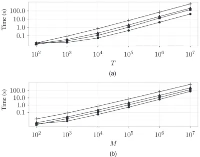
Fig. 3 shows execution times for the implementation of algorithm 2, the NOT solution path algorithm, implemented in the R packagenot, with the data{Yt}tT=1being IIDN.0, 1/. The
(a) T ime (s) T ime (s) (b)
Fig. 3. Execution times for the implementation of algorithm 2 available in R package not (Baranowski et al., 2016a), for various feature detection problems with the dataYt,tD1,. . . ,T, IIDN.0, 1/(in a single run, computations for the input of the algorithm are performed in parallel, using eight cores of an Intel Xeon 3.6-GHz central processor unit with 16 Gbytes of random-access memory; the computation times are averaged over 10 runs in each case) ( , scenario 1; , scenario 2; , scenario 3; , scenario 4): (a) fixedMD10000; (b) fixedTD10000
running times appear to scale linearly both inT (Fig. 3(a)) and inM(Fig. 3(b)), which pro-vides evidence that the computational complexity of algorithm 2 in this particular example is practically of orderO.MT/.
Finally, we remark that the memory complexity of algorithm 2 is alsoO.MT/, which combined with its low computational complexity implies that our approach can handle problems of size T in the range of millions.
3.6. Other practical considerations 3.6.1. Choice ofM
As can be seen in theorem 1 and theorem 2, the minimum required value forMgrows withT(i.e. atO{log.T/}, for a fixed number of well-spaced change points). In practice, when the number of observations is of the order of thousands, we would recommend settingM=10000. With this value ofM, the implementation of algorithm 1 provided in the Rnotpackage (Baranowski
et al., 2016a) achieves an average computation time not longer than 2 s in all the examples in Section 5 by using a single core of an Intel Xeon 3.6-GHz central processor unit. This can be accelerated further, as the notpackage allows for computing the contrast function over the intervals drawn in parallel by using all available central processor unit cores.
However, caution must be exercised for signals with a large expected number of change points, for whichMmay need to be increased. For example, Maidstoneet al.(2017) found that the NOT algorithm withM=105 offered better practical performance on the change point rich signals that they considered. In the most extreme scenario where we expect change points to occur very frequently with a largeT, we would recommend pickingMas large as possible to match the available computational power and applying a penalty that is less stringent than sSIC. See section F of the on-line supplementary materials.
3.6.2. Early stopping for narrowest-over-threshold method with the strengthened Schwarz information criterion
If the number of change points in the data is expected to be quite moderate, then it may not be necessary to calculate sSIC for allk. In practice, solutions on the path corresponding to very small values ofζT contain many estimated change points. Such solutions are unlikely to minimize equation (11). By considering|T.ζT.k//|qmax, we could achieve some computational gains without adversely impacting the overall performance of the methodology. As such, in all applications that are presented in this work we compute sSIC only forksuch that|T.ζT.k//|qmax withqmax=25.
4. Narrowest-over-threshold method under different noise types
In this section, we discuss how the NOT method can be extended to handle different types of noise. Section 4.1 deals with dependent noise, whereas Section 4.2 covers heavy-tailed noise. In addition, we investigate the case of noise with slowly varying variance in section D of the on-line supplementary materials.
4.1. Narrowest-over-threshold method under dependent noise
When the errors"tin model (3) are dependent withE."t/=0 and var."t/=1, the aforementioned NOT procedure can still be applied as a quasi-likelihood-type procedure. Conceivably, using the NOT algorithm here would incur information loss. As is shown in corollaries 1 and 2 in scenarios 1 and 2, the NOT method is still consistent if we replace the noise’s assumption of IID data in theorems 1 and 2 by stationarity with short memory. This new dependence assumption is satisfied by a large class of stationary time series models, including auto-regressive moving average models. See also the numerical examples in section E of the on-line supplementary materials, where we again select the thresholds automatically via sSIC. Here we assume that
σ0=1. However, if not, MAD-type estimators based on simple differencing are no longer appropriate for dependent data. We comment on this issue later. The following corollaries give guidelines on the choice of the threshold, as well as a guarantee on the performance of the NOT algorithm from a theoretical perspective.
Corollary 1. Suppose thatYtfollow model (3) in scenario 1, but with{"t}being a stationary short memory Gaussian process, i.e. the auto-correlation function of{"t}, denoted byρkfor any lagk∈Z, satisfiesΣ∞k=−∞|ρk|<∞. Then, the conclusion of theorem 1 still holds (with different
constants).
Corollary 2. Suppose thatYtfollow model (3) in scenario 2, but with{"t}being a stationary short memory Gaussian process. The conclusion of theorem 2 holds (with different constants). In our theoretical development for the dependent noise setting, the smallest permitted thresh-old to be used in the NOT algorithm depends linearly onσ0.Σ∞k=−∞|ρk|/1=2. This quantity can
also be viewed as a generalization of the independent noise setting, where the threshold is pro-portional toσ0(sinceΣ∞k=−∞|ρk| =1). More details of its derivation are provided in section 1.6
of the on-line supplementary materials.
This poses a few challenges in the practical application of NOT detection to signals with dependent noise:
(a) the (pre-)estimation of the residuals"tin preparation for the estimation of their long-run variance;
(c) the estimation ofσ0.Σ∞k=−∞|ρk|/1=2.
These problems are known to be difficult in time series analysis in general. A possible solution is outlined below.
For problem (a), we have had some success with the wavelet-based method of Johnstone and Silverman (1997), which was implemented in the R packagewavethresh(Nason, 2016); its advantages are that it is specifically designed for dependent noise and that, being based on non-linear wavelet shrinkage, it is particularly suited for signals with irregularities, such as (generalized) change points. Here the Haar wavelet transform of the data is appropriate in scenario 1, whereas a transform with respect to any wavelet that annihilates linear functions is appropriate in scenarios 2 and 3. Once the empirical residuals have been obtained from problem (a) we could then estimateσ0in problem (b) by its sample version and estimateσ0.Σk∞=−∞|ρk|/1=2
in problem (c) in a model-based way (e.g. using the auto-regressive model with its orderpchosen by an information criterion).
Another possibility to estimate change points under dependent noise is to use self-normalizing-based statistics. See, for instance, Shao and Zhang (2010), Betken (2016), Peˇsta and Wendler (2018) and Zhang and Lavitas (2018). These statistics could potentially be fed into our NOT approach as well.
Finally, we mention two practical ways of reducing the dependence and making the series closer to Gaussian, before applying NOT detection:
(a) preaverage the data over non-overlapping moving windows of sizeh, creating a new data set of length⌊T=h⌋; the hope is that, by the law of large numbers, the preaveraged noise will be closer to Gaussian and also less serially dependent than the original noise; (b) add additional IID Gaussian noise to the data, with mean 0 and suitably chosen standard
deviation; this will have a similar effect to that previously, i.e. it will bring the distribution of the data closer to Gaussian and reduce the serial dependence within the data.
4.2. Extension of narrowest-over-threshold method under heavy-tailed noise
NOT detection appears to be relatively robust under noise misspecification. As is demonstrated later in Section 5, it offers reasonable estimates when the noise is non-Gaussian but the Gaussian contrast functions are used. We now discuss how its performance can be improved further in the presence of heavy-tailed noise.
In scenario 1, we propose to apply the following new contrast function, which is defined for
Yand 0s < b < eT as
˜
Cb.s,e].Y/= S.s,e].Y/,ψb.s,e] .12/ in our NOT procedure. Here, for any vectorv=.v1,: : :,vT/′, thei-component ofS.s,e].v/is given byS.s,e].v/i=sgn{vi−.e−s/−1Σet=s+1vt}andψb.s,e]is defined by equation (5). (For certain noise distributions, subtracting the sample median ofvinstead of the sample mean would appear more
appropriate.) The rationale behind function (12) is to assign Ys+1− 1 e−s e t=s+1 Yt,: : :,Ye− 1 e−s e t=s+1 Yt
(i.e. residuals for fitting a curve with no change point on a given interval) into two classes (±1, i.e. a two-point distribution, thus with light tails) and apply the contrast function to their±1-labels. The empirical performance of the NOT approach (via algorithm 2) combined with equation (12) and sSIC is also illustrated in section E of the on-line supplementary materials.
5. Simulation study
5.1. Settings
We consider examples following scenarios 1–4 that were introduced in Section 2.3, as well as an extra example satisfyingσt=σ0andftis a piecewise quadratic function oft(scenario 5).
We simulate data according to equation (3) by using the test signals M1 teeth, M2 blocks, M3 wave1, M4 wave2, M5 mix, M6 vol and M7 quad, with the noise following
(a) IIDN.0, 1/, (b) IIDN.0, 2/,
(c) IID scaled Laplace with zero mean and unit variance, (d) IID scaled Studentt5-distribution with unit variance and
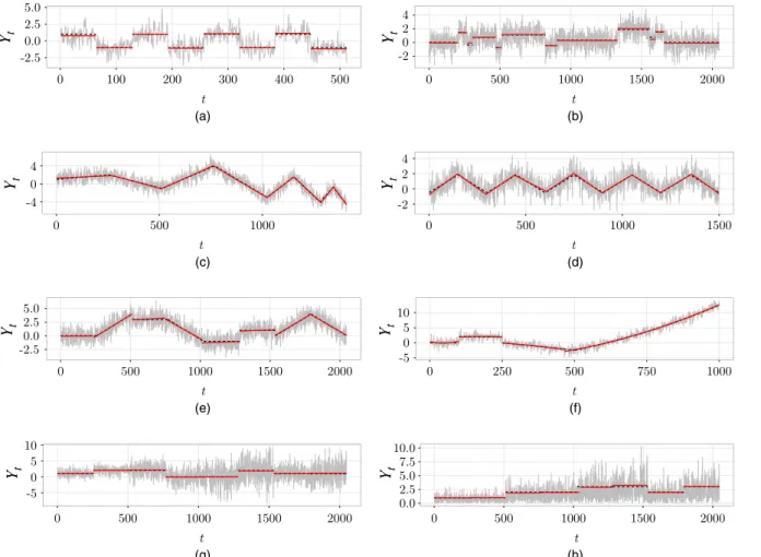
(e) a stationary Gaussian AR(1) process ofϕ=0:3, with zero mean and unit variance. A detailed specification of our test models can be found in section A of the on-line supplementary materials. Fig. 4 shows the examples of the data generated from models M1–M7, as well as the estimates produced by the NOT algorithm in a typical run.
5.2. Estimators
We apply algorithm 2 to compute the NOT solution path and pick the solution minimizing sSIC introduced in Section 3.3 withα=1 (which is equivalent to the Schwarz information criterion). In each simulated example, we use the contrast function that was designed to detect change points in the scenario that the example follows, given in Section 2.3 and section B of the on-line supplementary materials under the assumption that"tis IID Gaussian. The resulting method is referred to simply as ‘NOT’. In addition, for scenario 1 only, we also apply algorithm 2 combined with equation (12) and the Schwarz information criterion, which we call ‘NOT HT’. Here ‘HT’ stands for ‘heavy tails’. The number of intervals drawn in the procedure and the maximum number of change points for the Schwarz information criterion are set toM=10000 andqmax=25 respectively.
We then compare the performance of NOT and NOT HT against the best competitors avail-able in the Comprehensive R Archive Network. To the best of our knowledge, none of the competing packages can be applied in all of scenarios 1–5.
For change point detection in the mean, the selected competitors from the Comprehen-sive R Archive Network arechangepoint (Killick and Eckley, 2014; Killicket al., 2016) implementing the PELT methodology that was proposed by Killick, Fearnhead and Eckley (2012),changepoint.np(Hayneset al., 2016) implementing a non-parametric extension of the PELT methodology that was studied in Hayneset al.(2017),wbs(Baranowski and Fry-zlewicz, 2015) implementing WBS proposed by Fryzlewicz (2014),ecp(James and Matteson, 2014) implementing the e.cp3o method that was proposed by James and Matteson (2015),
strucchange(Zeileiset al., 2002) implementing the methodology of Bai and Perron (2003),
Segmentor3IsBack(Cleynenet al., 2013) implementing the technique that was proposed by Rigaill (2015),nmcdr(Zou and Lancezhange, 2014) implementing NMCD, the non-parametric multiple change point detection methodology of Zouet al.(2014),stepR(Peinet al., 2018) implementing the simultaneous multiscale change point estimator SMUCE that was proposed by Fricket al.(2014) andFDRSeg(Liet al., 2017) implementing the method called FDRSeg proposed by Liet al.(2016). We refer to the corresponding methods as PELT, NP-PELT, WBS, e.cp3o, B&P, S3IB, NMCD, SMUCE and FDRSeg respectively.
Note that e-cp3o, NMCD, NOT, PELT and NP-PELT can be used also for change point detection in scenario 4, where change points occur in the mean and variance of the data. In
Narro w est-o ver-threshold Detection 665 (a) (b) (c) (d) (e) (f) (g) (h) Y Yt Yt Yt Y Yt Yt Yt
Fig. 4. Examples of data generated from simulation models outlined in section A of the on-line supplementary materials: (a)–(g) data seriesYt( ), true signalft( ), ˆftbeing the least squares estimate offtwith the change points estimated by the NOT algorithm ( ); (h) centred datajYt fˆtj ( ), true standard deviationσt( ) and the estimated standard deviation ˆσtbetween the change points detected by the NOT algorithm ( ); (a) model M1 teeth, scenario 1; (b) model M2 blocks, scenario 1; (c) model M3 wave1, scenario 2; (d) model M4 wave2, scenario 2; (e) model M5 mix, scenario 3; (f) model M7 quad, scenario 5; (g) model M6 vol,ft, scenario 4; (h) model M6 vol,σt, scenario 4
addition, for scenario 4, we also include the heterogeneous SMUCE method (Peinet al., 2017) implemented instepR(Peinet al., 2018) and the segment neighbourhoods method (Auger and Lawrence, 1989) implemented inchangepoint(Killick and Eckley, 2014; Killicket al., 2016). We refer to them as HSMUCE and SegNeigh respectively.
Only B&P allows for change point detection in piecewise linear and piecewise quadratic signals (in particular, WBS is not suitable for these settings as described in Sections 1 and 2.5); hence we also study the performance of the trend filtering methodology of Kimet al.(2009) termed TF hereafter, using the implementation that is available from the R packagegenlasso(Taylor and Tibshirani, 2014), to have a broader comparison. See also Linet al.(2017). TF aims to estimate a piecewise polynomial signal from the data, not focusing on the change point detection problem directly. Let ˆf.tTF/denote the TF estimate of the true signalft; then the TF estimates of the change points in scenario 2 are defined as thoseτfor which|2 ˆf.τTF/−fˆτ.TF−1/−fˆτ.TF+1/|>ǫ, where
ǫ>0 is a very small number being the numerical level of tolerance (more precisely, we set
ǫ=1:11×10−15 in our study). In the piecewise quadratic case, the change points are defined as thoseτ for which the third-order differences|fˆτ.TF+2/−3 ˆf.τTF+1/+3 ˆf.τTF/−fˆ.τTF−1/|>ǫ. We note that both B&P and TF require a substantial amount of computational resources in this study.
Finally, we remark that the tuning parameters for the competing methods are set to the values that were recommended by the corresponding R packages, and the R code for all simulations can be downloaded from our GitHub repository (Baranowskiet al., 2016b).
5.3. Results
Here we present only the results under the setting where the noise is (a) IID standard normal in Table 2. Additional results under the other above-mentioned noise settings can be found in section E of the on-line supplementary materials.
For each method, we show a frequency table for the distribution of ˆq−q, where ˆq is the number of the estimated change points andq denotes the true number of change points. We also report Monte Carlo estimates of the mean-squared error of the estimated signal, given by
MSE=E 1 T T t=1 .ft−fˆt/2 :
For all methods except TF, ˆftis calculated by finding the least squares approximation of the sig-nal of the appropriate type depending on the trueft, between each consecutive pair of estimated change points. For TF, ˆftused in the definition of the mean-squared error is the penalized least squares estimate offtreturned by the TF algorithm.
To assess the performance of each method in terms of the accuracy of the estimated locations of the change points, we report estimates of the (scaled) Hausdorff distance
dH=T−1E[max{ max
j=0,:::,q+1k=0,min:::, ˆq+1|τj−τˆk|,k=max0,:::, ˆq+1j=0,min:::,q+1|τˆk−τj|}],
where 0=τ0<τ1< : : : <τq<τq+1=T and 0=τˆ0<τˆ1< : : : <τˆq<τˆq+1=T denote respectively true and estimated locations of the change points. From the definition above, it follows that 0dH1. An estimator is regarded as performing well when itsdHis close to 0. However,dH would be large when the number of change points is underestimated or some of the estimated change points are far from the real change points. In addition, we also report estimates of the inverseV-measuredV defined as
where ‘V.·,·/’ is theV-measure (withβ=1) proposed by Rosenberg and Hirschberg (2007) for the evaluation of segmentation. An estimator is regarded as performing well when itsdVis close to 0. More specifically, 0dV1, and a perfect estimator hasdV=0, whereasdV=1 means that none of the features are detected (i.e. ˆq=0).
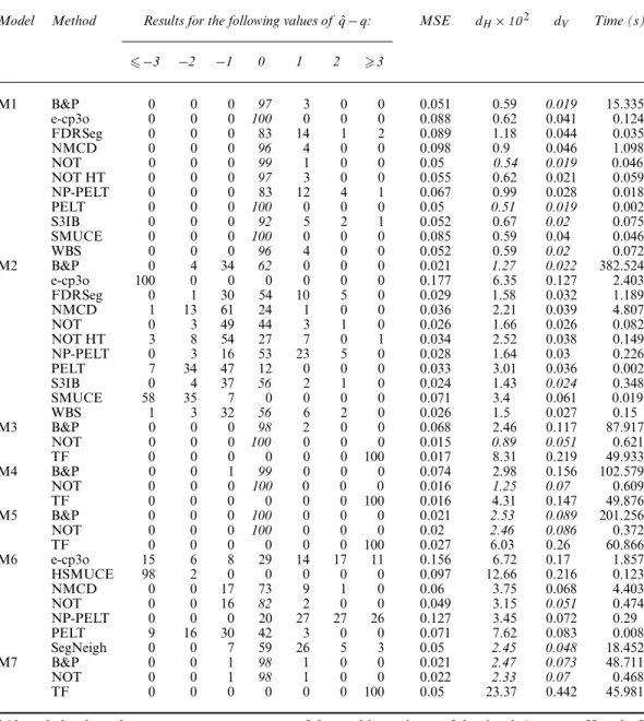
We find that, in most of the simulated scenarios, the NOT method is among the most compet-itive methods in terms of the estimation of the number of change points and their locations, as well as the true signal. Importantly, it is very fast to compute, which gives it a particular advan-tage over its competitors in scenarios 2, 3 and 5. Finally, the NOT algorithm with the contrast function derived under the assumption that the noise is IID Gaussian is relatively robust against the misspecification in"t, when the truth is either correlated or heavy tailed.
6. Real data analysis
6.1. Temperature anomalies
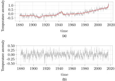
We analyse the Goddard Institute for Space Studies surface temperature anomalies data set that is available from GISTEMP Team (2016) (http://data.giss.nasa.gov/gistemp /tabledata v3/GLB.Ts+dSST.csv), consisting of monthly global surface temperature anomalies recorded from January 1880 to June 2016. The anomaly here is defined as the dif-ference between the average global temperature in a given month and the baseline value, being the average calculated for that time of the year over the 30-year period from 1951 to 1980; for more details see Hansenet al.(2010). This and similar anomalies series are frequently studied in the literature with a particular focus on identifying change points in the data; see for example Ruggieri (2013) or James and Matteson (2015).
The plot of the data (Fig. 5(a)) indicates the presence of a linear trend with several change points in the temperature anomalies series. The corresponding changes are not abrupt; therefore we believe that scenario 2 with change points in the slope of the trend is the most appropriate here. To detect the locations of the change points, we apply the NOT algorithm (via algorithm 2) with the contrast given by equation (8), combined with the Schwarz information criterion to determine the best model on the solution path.
(a) T emperature anomaly T emperature anomaly (b)
Fig. 5. Change point analysis for the GISTEMP data set introduced in Section 6.1: (a) data seriesYt( ) and ˆftestimated by using change points returned by the NOT algorithm ( ); (b) residuals ˆ"tDYt fˆt
Table 2. Distribution of ˆq qfor data generated according to model (3) with the noise term"tIIDN.0, 1/ for various choices offt andσtgiven in section A of the on-line supplementary materials and competing methods listed in Section 5†
Model Method Results for the following values ofqˆ−q: MSE dH×102 dV Time (s)
−3 −2 −1 0 1 2 3 M1 B&P 0 0 0 97 3 0 0 0.051 0.59 0.019 15.335 e-cp3o 0 0 0 100 0 0 0 0.088 0.62 0.041 0.124 FDRSeg 0 0 0 83 14 1 2 0.089 1.18 0.044 0.035 NMCD 0 0 0 96 4 0 0 0.098 0.9 0.046 1.098 NOT 0 0 0 99 1 0 0 0.05 0.54 0.019 0.046 NOT HT 0 0 0 97 3 0 0 0.055 0.62 0.021 0.059 NP-PELT 0 0 0 83 12 4 1 0.067 0.99 0.028 0.018 PELT 0 0 0 100 0 0 0 0.05 0.51 0.019 0.002 S3IB 0 0 0 92 5 2 1 0.052 0.67 0.02 0.075 SMUCE 0 0 0 100 0 0 0 0.085 0.59 0.04 0.046 WBS 0 0 0 96 4 0 0 0.052 0.59 0.02 0.072 M2 B&P 0 4 34 62 0 0 0 0.021 1.27 0.022 382.524 e-cp3o 100 0 0 0 0 0 0 0.177 6.35 0.127 2.403 FDRSeg 0 1 30 54 10 5 0 0.029 1.58 0.032 1.189 NMCD 1 13 61 24 1 0 0 0.036 2.21 0.039 4.807 NOT 0 3 49 44 3 1 0 0.026 1.66 0.026 0.082 NOT HT 3 8 54 27 7 0 1 0.034 2.52 0.038 0.149 NP-PELT 0 3 16 53 23 5 0 0.028 1.64 0.03 0.226 PELT 7 34 47 12 0 0 0 0.033 3.01 0.036 0.002 S3IB 0 4 37 56 2 1 0 0.024 1.43 0.024 0.348 SMUCE 58 35 7 0 0 0 0 0.071 3.4 0.061 0.019 WBS 1 3 32 56 6 2 0 0.026 1.5 0.027 0.15 M3 B&P 0 0 0 98 2 0 0 0.068 2.46 0.117 87.917 NOT 0 0 0 100 0 0 0 0.015 0.89 0.051 0.621 TF 0 0 0 0 0 0 100 0.017 8.31 0.219 49.933 M4 B&P 0 0 1 99 0 0 0 0.074 2.98 0.156 102.579 NOT 0 0 0 100 0 0 0 0.016 1.25 0.07 0.609 TF 0 0 0 0 0 0 100 0.016 4.31 0.147 49.876 M5 B&P 0 0 0 100 0 0 0 0.021 2.53 0.089 201.256 NOT 0 0 0 100 0 0 0 0.02 2.46 0.086 0.372 TF 0 0 0 0 0 0 100 0.027 6.03 0.26 60.866 M6 e-cp3o 15 6 8 29 14 17 11 0.156 6.72 0.17 1.857 HSMUCE 98 2 0 0 0 0 0 0.097 12.66 0.216 0.123 NMCD 0 0 17 73 9 1 0 0.06 3.75 0.068 4.403 NOT 0 0 16 82 2 0 0 0.049 3.15 0.051 0.474 NP-PELT 0 0 0 20 27 27 26 0.127 3.45 0.072 0.29 PELT 9 16 30 42 3 0 0 0.071 7.62 0.083 0.008 SegNeigh 0 0 7 59 26 5 3 0.05 2.45 0.048 18.452 M7 B&P 0 0 1 98 1 0 0 0.021 2.47 0.073 48.711 NOT 0 0 1 98 1 0 0 0.022 2.33 0.07 0.468 TF 0 0 0 0 0 0 100 0.05 23.37 0.442 45.981
†Also tabulated are the average mean-square error of the resulting estimate of the signalft, average Hausdorff distancedH, average inverse V-measuredV and average computation time by using a single core of an Intel Xeon 3.6-GHz central processor unit with 16 Gbytes of random-access memory, all calculated over 100 simulated data sets. Methods with the largest empirical frequency of ˆq−q=0 or smallest average ofdHordV, and those within 10% of the highest or lowest accordingly, are given in italics.
Narro w est-o ver-threshold Detection 669 (b) (e) (c) (f)
Monthly percentage change Monthly percentage change
Fig. 6. Change point analysis for the monthly percentage changes in the UK HPI from January 1995 to May 2016: (a)–(c) monthly percentage changes Ytand the fitted piecewise constant mean ˆft, between the change points estimated with the NOT method; (d)–(f)jYt fˆtjand the fitted piecewise constant standard deviation ˆσt, between the change points estimated with the NOT method; (a), (d) Hackney; (b), (e) Newham; (c), (f) Tower Hamlets
The NOT estimate of the piecewise linear trend and the corresponding empirical residuals are shown in Fig. 5. We identify eight change points at the following dates: March 1901, December 1910, July 1915, June 1935, April 1944, December 1946, June 1976 and May 2015. Previous studies, conducted on similar temperature anomalies series (observed at a yearly frequency and obtained from a different source), report change points around 1910, 1945 and 1976 (see Ruggieri (2013) for an overview of some related analyses). In addition to the change points around these dates, the NOT algorithm identifies two periods, 1901–1915 and 1935–1946, with local deviations from the baseline. We also observe a long-lasting upward trend in the anomalies series starting in December 1946. Finally, NOT detection indicates that the slope of the trend is increasing, with the most recent change point in May 2015.
6.2. UK house price index
We analyse monthly percentage changes in the UK house price index (HPI) (https://www. gov.uk/government/statistical-data-sets/uk-house-price-index-data-downloads-january-2017), which provides an overall estimate of the changes in house prices across the UK. The data and a detailed description of how the index is calculated are available on line from UK Land Registry (2016). Fryzlewicz (2018b), who proposed a method for signal estimation and change point detection in scenario 1, used this data set to illustrate the performance of his methodology. We perform a similar analysis, assuming the more flexible scenario 4, allowing for changes both in the mean and in the variance, which, we argue, leads to additional insights and better interpretable estimates for this data set.
As in Fryzlewicz (2018b), we analyse the percentage changes in the HPI for three London boroughs, namely Hackney, Newham and Tower Hamlets, all of which are in East London. Hackney and Tower Hamlets border on the City of London, which is a major business and financial district, and home to Canary Wharf, which is another important financial centre. In contrast Newham, to the east of Hackney and Tower Hamlets, hosted the London 2012 Olympic Games, which involved large-scale investment in that borough.
Fig. 6 shows monthly percentage changes in the HPI for the boroughs analysed and the corresponding NOT estimates, obtained by using the contrast function for scenario 4. As rec-ommended in Section 3.3, we set the number of intervals drawn in the procedure toM=10000 and choose the threshold that minimizes the Schwarz information criterion. For better compa-rability, the NOT algorithm is applied with the same random seed for each data series.
In contrast with Fryzlewicz (2018b), whose tail greedy unbalanced Haar method estimates at least 10 change points in each HPI series, we detect just a few change points in the data, facili-tating the interpretation of the results. Furthermore, for all three boroughs, the NOT algorithm estimates two change points (one around March 2008 and one around September 2009) that could possibly be linked to the 2008–2009 financial crisis and its effect on the housing market. Estimated standard deviations for that period are much larger than the estimates corresponding to the other segments of piecewise constancy, suggesting that the market is more volatile during 2008–2009, and thus in this example scenario 4 may be more relevant than scenario 1 considered in Fryzlewicz (2018b).
Acknowledgements
We thank Paul Fearnhead for his helpful comments on an earlier draft, and on the implementa-tion of our R package. We also thank the Associate Editor and four referees for their comments and suggestions. Piotr Fryzlewicz’s work was supported by Engineering and Physical Sciences Research Council grant EP/L014246/1.

![Fig. 2. Plots of (a) ψ b .s,e] and (b) φ b .s,e] given by respectively equation (5) and equation (7) for s D 0, e D 1000 and several values of b: , b D 125; , b D 500; , b D 750](https://thumb-us.123doks.com/thumbv2/123dok_us/9040332.2801834/8.727.88.663.384.895/fig-plots-ψ-given-respectively-equation-equation-values.webp)