Markov chain Monte Carlo methodoloy for inference with generalised linear spatial models

(1)

Markov Chain Monte Carlo

methodology for inference

with generalised linear spatial

models

Ioanna Lampaki

Submitted for the degree of Doctor of Philosophy at Lancaster University,

(2)

(3)

(4)

Declaration

I declare that this thesis entitled ”MCMC methodology for inference on generalised linear spatial models” is the result of my own research under the guidance of Dr. Chris Sherlock except as otherwise cited in the references. This thesis has not been submitted in any form for the award of a higher degree elsewhere.

All the algorithms presented in Chapter 3 have been coded in R (R Core Team 2015) whereas the algorithms presented in Chapter 4 have been coded in the C programming language using the GNU Scientific Library (Galassi et al. 2010).

(5)

Acknowledgements

This doctoral thesis was funded by the Faculty of Science and Technology of Lancaster University and many people have contributed to its completion in so many different ways. First and foremost, I would like to express my gratitude to my supervisor Chris Sherlock for his guidance and support. His help, intuition and excitement has been invaluable for the completion of this thesis. I would especially like to thank him for his patience, willingness and ability to always give answers to my never-ending questions. Working with him has been an invaluable experience and has taught me a lot. I am also indebted to him for proofreading this thesis and providing me with constructive comments. I would also like to thank Jonathan Tawn for his genuine interest and support.

I have been very lucky in sharing the same office for four years with some of the most wonderful people I have ever met. Special mention to Stephanie Wallace, Ross Towe, Karen Pye and my ”neighbour” Simon Taylor who was always willing to help with any problem I had while I was learning to code in C. You have all been such a great company, supporters, office-mates and source of laugh and joy throughout these years. I would also like to thank Giorgos Sermaidis, Yanyun Wu and Ye Liu for all the good time we had.

(6)

My time in Lancaster would not have been the same without you. All of you are part of my best memories in Lancaster. A big thanks to Ioannis Papastathopoulos for his continuous encouragement and emotional support during this journey.

Lastly but definitely not least, the biggest thank you goes to my family, Vasilis, Tina, Liza and Eleni for their endless support and love. Also, to my adorable nieces, Agapi and Ioli for always making me eager to visit home and for making me understand that sometimes there might be more important things than this work out there. I wouldn’t have made it without you. Thank you!

(7)

Abstract

Many real world phenomena are described through models that include an unobserved process which is usually characterised by a continuous distribution. Such models are widely used in geostatistics where a continuous spatial phenomenon is modelled through an underlying latent Gaussian process.

If the observed data are also Gaussian then inference for the underlying process and the model parameters is relatively straightforward. In many applications though the as-sumption of normally distributed data is not sensible and the asas-sumption of Poisson or binomial data is more suitable. These models, with non-Gaussian data, are known as generalised linear spatial models (GLSM). In such cases, inference requires more so-phisticated techniques and a common approach is the use of Markov chain Monte Carlo methods (MCMC). However, the correlation between the components of the latent pro-cess and the correlation between the latent propro-cess and the model parameters generally hinders the performance of any MCMC scheme which updates the latent process and the parameters sequentially.

(8)

In this thesis we focus on the Poisson GLSM and elaborate on the problem of the correla-tion within the latent process. In particular, our aim is to construct an efficient proposal distribution for sampling from the posterior distribution of the latent process condition-ally on the other parameters. Initicondition-ally, we investigate the idea of constructing a global normal approximation to the conditional posterior distribution of the latent process and use it as the proposal distribution in a simple and fast MCMC scheme. For this purpose, we initially employ various transformations of the data and find that some of the con-structed schemes perform well in certain low dimensional scenarios. Subsequently, we construct one dimensional proposals for each component of the latent process through an approximation to each univariate marginal posterior conditional on a few principal components. The suggested MCMC scheme updates each component of the process sep-arately and then proceeds by updating the few important principal components. As suggested by our results, this method has a stable and efficient performance in a variety of scenarios and dimensions.

(9)

List of Tables

3.3.1 Algorithm L1. Acceptance rates (α), relative ESS, average CPU time

and adjusted ESS for dimensions d = 25,49,100. Grey color indicates

that the permutation test does not support convergence. The∗ indicates

that the thinned sample size was less than 50 and permutation test was

not conducted. . . 86

3.3.2 Algorithm L2. Acceptance rates (α), relative ESS, average CPU time

3.3.3 Algorithm A1. Acceptance rates (α), relative ESS, average CPU time

(13)

3.3.4 Algorithm RA. Acceptance rates (α), relative ESS, average CPU time

3.3.5 Algorithm iRA. Acceptance rates (α), relative ESS, average CPU time

3.3.6 Algorithm Christensen et al. (2006). Acceptance rates (α), relative ESS,

average CPU time and adjusted ESS for dimensionsd= 25,49,100. . . 91

3.3.7 Algorithm pMMALA. Acceptance rates (α), relative ESS, average CPU

time and adjusted ESS for dimensionsd= 25,49,100. . . 92

4.3.1 Algorithm U-MHIS. Minimum, median and maximum acceptance rates

(α), relative ESS, average CPU time and adjusted ESS for dimensions

d={25,49,100}. Grey colour: K–S test does not support convergence. . . 134

4.3.2 U-PC. Minimum, median and maximum acceptance rates (α), relative

ESS, average CPU time and adjusted ESS for dimensionsd={25,49,100}.

Grey colour: K–S test does not support convergence. . . 135

4.3.3 PC-RWM. Minimum, median and maximum acceptance rates (α), relative

ESS, average CPU time and adjusted ESS for dimensionsd= 25,49,100.

(14)

4.3.4 PC-MALA. Minimum, median and maximum acceptance rates (α),

rel-ative ESS, average CPU time and adjusted ESS for dimensions d =

{25,49,100}. Grey colour: K–S test does not support convergence. . . 137

4.3.5 Algorithm Christensen et al. (2006). Relative ESS, average CPU time

and adjusted ESS for dimensions d = {25,49,100}. The algorithm was

tuned so that it achieved acceptance rates 57%−59%. . . 138

4.3.6 Algorithm of Christensen et al. (2006) and PC-MALA. Minimum, median

and maximum acceptance rates (α), relative ESS, average CPU time and

adjusted ESS for dimension d = 196. Grey: KS test does not support

convergence. . . 139 4.3.7 Algorithm of Christensen et al. (2006) and PC-MALA. Minimum, median

and maximum acceptance rates (α), relative ESS, average CPU time and

adjusted ESS for dimension d = 400. Grey: KS test does not support

convergence. . . 140 4.3.8 Algorithm of PC-MALA (left) and Christensen et al. (2006) (right).

Min-imum, median and maximum acceptance rates (α), relative ESS, average

CPU time and adjusted ESS for dimensions d= 25,49,100. The

accep-tance rates displayed correspond to PC-MALA. Grey: KS test does not

support convergence. The correlation matrix R is constructed using the

(15)

4.3.9 Algorithm of PC-MALA (left) and Christensen et al. (2006) (right).

Min-imum, median and maximum acceptance rates (α), relative ESS, average

CPU time and adjusted ESS for dimensionsd= 196,400. The acceptance

rates displayed correspond to PC-MALA. Grey: KS test does not support

convergence. The correlation matrix R is constructed using the Matern

(16)

List of Figures

2.1 Density of the proposal distribution, q(θ) (dashed line) and of the target

distributionπ(θ) (solid line). . . 22

2.2 Correlation against distance. Left: exponential correlation function with

φ= 1, Right: Gaussian correlation function withφ= 1.73. The parameter

φhas been matched so that in both casesρ(u) = 0.05 at the same distance

u. . . 32

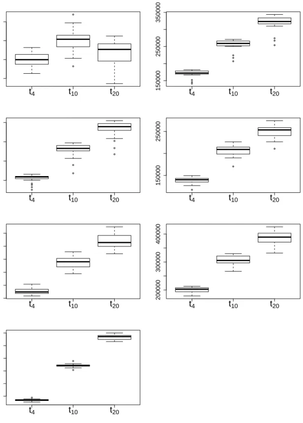
3.1 Boxplots of ESS obtained form algorithm L1 for seven different scenarios

of parameter values and dimension d= 25. . . 75

3.2 Contours of bivariate log-target (Black lines) and log-proposals (Red lines)

distribution. Top row: Proposals of the L1 (left) and L2 (right) algo-rithms. Middle row: Proposals of the RA (left) and iRA (right) proposals.

Bottom row: Proposal of A algorithm onηscale (left) andψ scale (right).

Parameters’ values fixed to be y = (10,10), µ_η = (log(10),log(10)),

(17)

3.3 Contours of bivariate log-target (Black lines) and log-proposals (Red lines) distribution. Top row: Proposals of the L1 (left) and L2 (right) algo-rithms. Middle row: Proposals of the RA (left) and iRA (right) proposals.

Bottom row: Proposal of A algorithm onηscale (left) andψ scale (right).

Parameters’ values fixed to be y = (10,10), µ_η = (log(10),log(10)),

σ2= 1, φ= 10 and distance between points set equal to 1. . . 95

3.4 Contours of bivariate log-target (Black lines) and log-proposals (Red lines)

distribution. Top row: Proposals of the L1 (left) and L2 (right)

algo-rithms. Middle row: Proposals of the A1 (left) and A2 (right)

algo-rithms onη scale. Bottom row: Proposals of the A1 (left) and A2 (right)

algorithms on ψ scale. Parameters’ values fixed to be y = (10,10),

µ_η = (log(10),log(10)), σ2 = 1, φ = 100 and distance between points

set equal to 1. . . 96

4.1 Plots of ¯va (grey solid line), ¯vt (black dashed line) and ¯vE _{(black solid}

line) against the numberkof principal components. The prior correlation

matrix R is constructed using the exponential correlation function. Top

to Bottom: d = {25,49,100,196,400}. Left to Right: φ = 1, φ = 10,

φ= 100. . . 120

4.2 Colour configuration for Figures 4.3–4.5 and Figure 4.7. Each colour

cor-responds to a different scenario of parameter values. . . 123

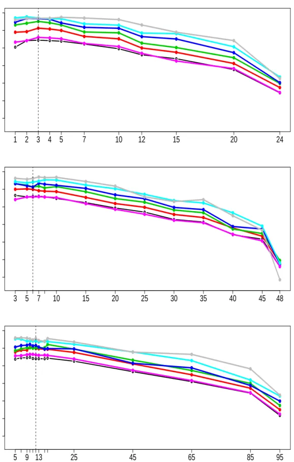
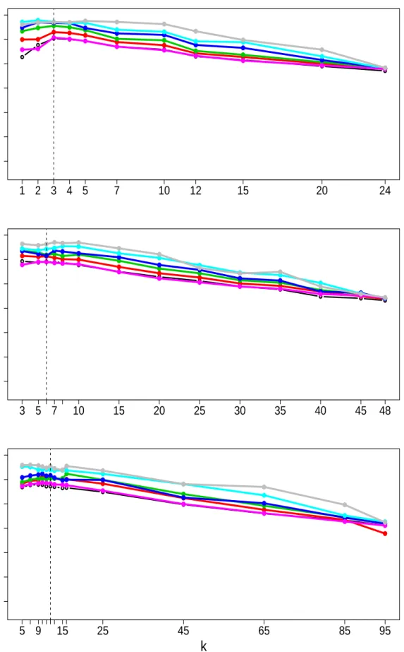
4.3 Algorithm U-PC. Logarithm of minimum relative ESS against different

values ofk. Top to bottom: Dimension,d={25,49,100}. The correlation

(18)

4.4 Algorithm PC-RWM. Logarithm of minimum relative ESS against

differ-ent values ofk. Top to bottom: Dimension,d={25,49,100}. The

corre-lation matrixR is constructed using the exponential correlation function. 125

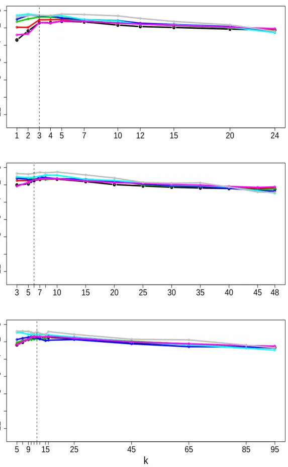
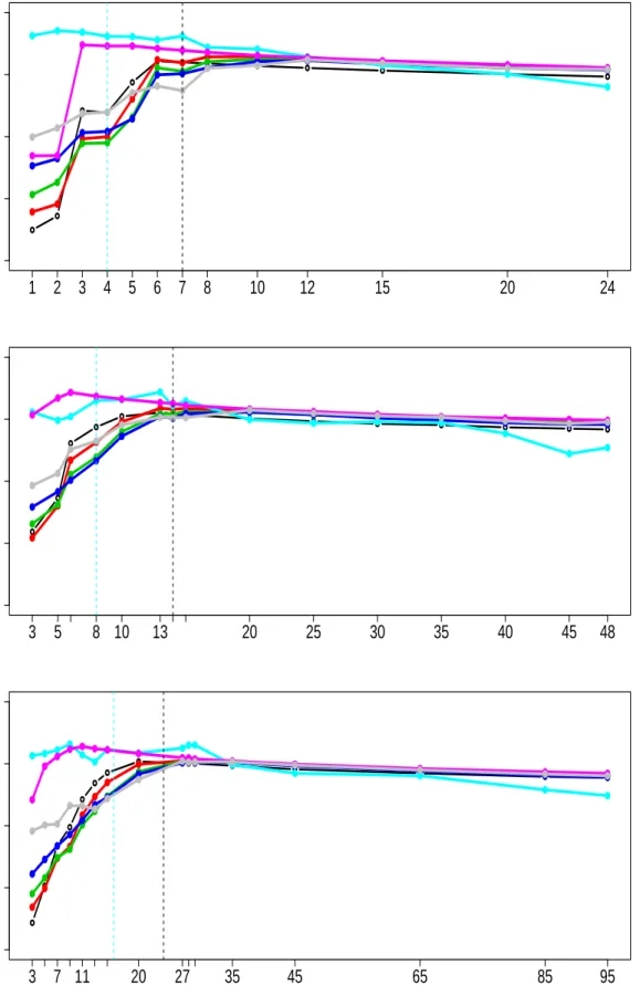
4.5 Algorithm PC-MALA. Logarithm of minimum relative ESS against

dif-ferent values ofk. Top to bottom: Dimension,d={25,49,100}. The

cor-relation matrixRis constructed using the exponential correlation function.126

4.6 Plots of ¯va _{(grey solid line), ¯}_vt _{(black dashed line) and ¯}_vE _{(black solid}

line) against the numberkof principal components. The prior correlation

matrix R is constructed using the Mat´ern family with κ = 1.5. Top to

Bottom:d={25,49,100,196,400}. Left to Right: φ={1,10,100} . . . 141

4.7 Algorithm PC-MALA. Logarithm of minimum relative ESS against

dif-ferent values of k. Top to bottom: Dimension, d = {25,49,100}. The

correlation matrixR is constructed using the Matern family with κ= 1.5. 142

4.8 Density plots of KS10, KS11, KS23 (left to right). The red lines indicate

the 95% quantile and the black dashed line the observed value of the

statistic. Scenario (d= 25,µ_η = log(10), σ2= 1, φ= 10,dataset b). . . 148

4.9 Density plots of KS7, KS12, KS20, KS48, KS49 (left to right). The red

lines indicate the 95% quantile and the black dashed line the observed

value of the statistic. Scenario (d = 49,µ_η = log(10), σ2 = 3, φ = 10,

dataset c). . . 149

4.10 Density plots ofKS3,KS8,KS33,KS41,KS71,KS90,KS93(left to right

and top to bottom). The red lines indicate the 95% quantile and the black

dashed line the observed value of the statistic. Scenario (d = 100,µ_η =

(19)

4.11 Plots of posterior means (left) and variances (right) of η. x-axis: Chris-tensen et al. (2006) algorithm, y-axis: U-PC algorithm. Top to Bottom:

scenario (d = 25, µ_η = log(10), σ2 = 1, φ = 10, dataset b), scenario

(d = 49, µ_η = log(10), σ2 _{= 3,} _φ _{= 10, dataset c), scenario (}_d _{= 100,}

µ_η = log(100), σ2 = 1,φ= 10, dataset a) . . . 152

4.12 QQ-plots of η10, η11, η23. x-axis: Algorithm of Christensen et al. (2006),

y-axis: U-PC algorithm. Scenario (d= 25,µ_η = log(10), σ2 _{= 1}_{, φ}_{= 10}_,

dataset b). . . 153

y-axis: U-PC algorithm. Scenario (d= 19,µη = log(10), σ2 = 1, φ= 10,

dataset b). . . 153

y-axis: U-PC algorithm. Scenario (d= 100,µ_η = log(10), σ2 = 1, φ= 10,

dataset b). . . 154

4.15 Traceplots for η10, η11, η23 (top to bottom) obtained from algorithm of

Christensen et al. (2006) (left) and U-PC algorithm (right). Scenario (d=

25,µ_η = log(10), σ2= 1, φ= 10,dataset b). . . 155

4.16 Traceplots forη7, η12, η20, η48, η49(top to bottom) obtained from algorithm

of Christensen et al. (2006) (left) and U-PC algorithm (right). Scenario

(d= 49,µ_η = log(10), σ2 = 3, φ= 10,dataset c). . . 155

4.17 Traceplots forη3,η8,η33,η41,η71,η90,η93(top to bottom) obtained from

algorithm of Christensen et al. (2006) (left) and U-PC algorithm (right).

(20)

4.18 Autocorrelation plots of η10, η11, η23 (left to right and top to bottom).

The black line corresponds to the ACF for the algorithm of Christensen et al. (2006) and the red line to U-PC. The dashed lines indicate the upper

and lower bounds of a 95% confidence interval. Scenario (d = 25,µ_η =

log(10), σ2 = 1, φ= 10, dataset b) . . . 156

4.19 Autocorrelation plots of η7, η12, η20, η48, η49 (left to right and top to

bot-tom). The black line corresponds to the ACF for the algorithm of Chris-tensen et al. (2006) and the red line to U-PC. The dashed lines indi-cate the upper and lower bounds of a 95% confidence interval. Scenario

(d= 49,µη = log(10), σ2 = 3, φ= 10, dataset c) . . . 157

4.20 Autocorrelation plots of η3, η8, η33, η41, η71, η90, η93 (left to right and

top to bottom).The black line corresponds to the ACF for the algorithm of Christensen et al. (2006) and the red line to U-PC. The dashed lines indicate the upper and lower bounds of a 95% confidence interval. Scenario

(21)

CHAPTER

1

Introduction

1.1 Motivation

Geostatistics is a branch of spatial statistics focusing on the study of a continuous spa-tial phenomenon. Such phenomena could be the temperature, radioactivity or even the intensity of weed growth over a predefined area of study. This kind of phenomena can conceptually be described by a continuous stochastic process, which however, is not di-rectly observed. Instead, what we have available is only a finite sample of observations of a random variable at specific locations over the study area. However, the locations of the data are not informative about the process we want to model. These observations, are usually assumed to be either identical to or a noisy version of the underlying true process or of a function of it. Interest usually lies in either predicting the realisation of the process at unsampled locations or making inference about the parameters of the model.

(22)

The typical modelling framework for such geostatistical problems is the generalised linear spatial model (GLSM). The GLSM is a generalised linear model but with an additional layer of stochasticity, the underlying latent process, in the linear predictor. The modelling of this process depends on the problem under study. It could for instance be modelled as a stationary or non-stationary Gaussian process, Gaussian Markov random field or we could even loosen the assumption of Gaussianity. In this Thesis we focus on the traditional GLSM as introduced in Diggle et al. (1998) where it is modelled through a stationary Gaussian process. The parameters involved in the model are of two types. Those used to model the trend and those used to model the spatial dependence, i.e., the covariance structure of the process. The GLSM gives the flexibility of modelling various types of data such as Poisson or binomial and also has as a special case the linear spatial model where the response variable is assumed to be normally distributed. In this thesis we deal with non-linear models and especially the Poisson GLSM.

Under the Bayesian framework, inference on the latent process and the parameters of the model relies on the use of MCMC methods since direct sampling from their joint posterior distribution is not possible; unless the data are Gaussian. Usually, in order to sample from this joint posterior an MCMC scheme will alternate between updating the parameters conditionally on the latent process and then updating the latent process conditionally on the current values of the parameters in the chain. Although such a scheme might appear straightforward to implement, it entails practical difficulties.

First of all, the latent process is usually of high dimension and this automatically hinders the performance of any MCMC scheme since mixing and convergence times increase with the dimension of the target; as also does their computational cost. Moreover, there is dependence between the latent process and the parameters and this will usually cause

(23)

the chain to converge and mix slowly. If the updating mechanism, say, for one of the parameters is not efficient this can also affect the mixing of the other components that are updated conditionally on that parameter.

Another challenging issue, is sampling from the posterior distribution of the latent pro-cess conditional on the parameters. The problem lies not only on the dependence of the latent process with the parameters but on the fact that the components of the process

can be strongly correlated ´a posteriori. This posterior dependence in combination with

the dimensionality of the process makes the construction of an efficient proposal chal-lenging. Updating the latent process in blocks can lead to poor mixing for the same reasons as explained in the previous paragraph. On the other hand, updating the latent process in one step is also demanding since a proposal distribution that aattempts to match the shape of a correlated high dimensional target is hard to construct.

All parameters affect how strong the posterior correlation within the latent process will be but a very important contributing factor is the data and more specifically the amount of information they provide on the latent process. For instance, if the data are weak then the main contribution to the posterior distribution of the process will come from the prior, and the posterior dependence can therefore be strong. On the other hand, if the data are strongly informative then the likelihood will contribute more to the posterior distribution and the components of the latent process will be approximately

independent´a posteriori or at least less correlated than´a priori. This is a key obstacle

in constructing a generic MCMC scheme that would perform efficiently irrespective of the observed data.

Christensen et al. (2006) have suggested an MCMC scheme that attempts to provide a solution to all of the aforementioned problems. Their approach is based on a

(24)

reparam-eterisation of the process and the mean parameters so that these are all approximately independent with zero mean and unit variance. Additionally, these transformed random variables are also expected to be approximately independent of the parameters associ-ated with the covariance structure of the process. They have provided a good, workable solution to the difficult problem of dependence between the latent process and the other parameters.

Finally, before closing this section we should mention that alternatives to MCMC meth-ods for inference on GLSMs do exist such as the more recently introduced approach of integrated nested Laplace approximation (INLA) (Rue et al. 2009). INLA is a method of approximate Bayesian inference and unlike traditional MCMC it is a non-sampling based technique and provides approximate inference through a series of accurate Gaus-sian and Laplace approximations. Another fundamental difference between INLA and MCMC is that the former assumes that inferences are to be drawn on the marginal posterior distributions of each component of the latent process and these exactly are the posteriors that it attempts to approximate. The procedure followed in order to approx-imate these posterior marginals can be briefly summarised in the following steps. First of all, the joint posterior distribution of the model parameters is approximated using the Laplace approximation and subsequently the marginal posterior of each parameter is obtained by numerically integrating out the remaining model parameters. Then, the marginal posterior distribution of each component of the latent process given the model parameters is approximated. This is achieved using a series expansion that takes into account third order terms that account for the skewness. Finally, the model parameters are integrated out of the product of the two marginal approximations in order to obtain the marginal posterior of each component of the latent process. Great computational

(25)

gains are achieved when the underlying latent process has a Markov structure as illus-trated in Rue et al. (2009). Although this is not required for the implementation of the suggested methodology, methods for approximating Gaussian processes through Gaus-sian Markov processes do exist Rue & Held (2005), Lindgren et al. (2011) and reduce the comptutauional complexity of the problem. For a comparative study between INLA and specfic MCMC methods we refer the reader to Taylor & Diggle (2012).

1.2 Scope and Outline

The focus of the present thesis is to provide an efficient MCMC scheme for inference on generalised linear spatial models. Since Christensen et al. (2006) have provided a framework for breaking the dependence between the process and the parameters we constrain our focus on the development of an efficient proposal for the latent process. Therefore, the methodology developed in Chapter 3 and Chapter 4 considers that all parameters in the model are fixed and interest lies only on sampling from the posterior distribution of the process given all the parameters. Although our focus is placed on the Poisson generalised linear spatial model, most of the proposed methodology could also be extended to the case of a Binomial generalised linear spatial model.

In Chapter 2 we provide material that is relevant and needed for the rest of the thesis. In Section 2.1 we outline some fundamental MCMC algorithms that will be used later on and discuss some issues related to their practical implementation, performance and efficiency. Section 2.2 introduces the reader to the area of geostatistics and the associated models. We describe the formulation and components of the linear spatial model along with the inferential procedure usually used and, in Section 2.2.6, extend these in the case of the generalised linear spatial model, which is the focus of this thesis. Finally, in

(26)

Section 2.2.7 we review some of the MCMC schemes that have been suggested in the literature for inference on the generalised linear spatial model.

In Chapter 3 we focus on constructing a single global normal approximation to the posterior density of interest. In particular, we explore the idea of applying a normal ap-proximation to the conditional density of a transformation of the data. This enables us to work under the framework of the linear Gaussian model, where the form of the posterior is tractable. In that way we are able to find an approximate posterior distribution for the latent variables and use this as a proposal in a simple, fast and straightforward-to-implement MCMC scheme.

In Chapter 4 we employ concepts of multivariate analysis and rather than constructing a global approximation to the target we use an approximation to each univariate marginal posterior conditional on a few principal components. In that way, we develop a two-stage proposal mechanism where each component of the process is updated separately and subsequently, the mixing of the algorithm is improved by additionally updating the few important principal components. This results in an efficient algorithm with stable performance across different datasets and dimensions.

Both in Chapter 3 and Chapter 4 the efficiency of the constructed algorithms is assessed and compared against existing schemes through extensive simulation studies.

(27)

CHAPTER

2

Background material

2.1 A review of Markov chain Monte Carlo algorithms

Markov chain Monte Carlo (MCMC) methods constitute a unified framework which enables sampling from complicated and analytically intractable distributions. This is achieved by constructing an ergodic Markov chain with stationary distribution identical to the distribution of interest. In our case this stationary distribution will be the posterior

distribution, π(θ|y), of a d-dimensional vector of continuous random variablesθ, given

the observed data,y. Once a sufficiently large sample is obtained, Monte Carlo estimates

of any functional ofθ, that we are interested in, can be obtained.

This section introduces the reader to the MCMC algorithms that are used in this thesis, namely the Metropolis-Hasting (MH), Random Walk Metropolis (RWM), Metropolis Adjusted Langevin Algorithm (MALA) and Riemann manifold MALA (MMALA) algo-rithm. In particular, we begin by setting out the basic MH algorithm and outline how the

(28)

rest are special cases of it. Theoretical properties and technical conditions for the con-vergence of these algorithms have been investigated over the last 20 years. However, we are mainly interested in their practical implementation and therefore focus on providing an intuitive interpretation of each algorithm and aspects that define their performance. Unless otherwise stated, the two main sources of this section are Gilks et al. (1996) and Gamerman & Lopes (2006).

2.1.1 Metropolis-Hastings algorithm (MH)

The MH algorithm, Metropolis et al. (1953) and Hastings (1970), uses an appropri-ate transition density such that the constructed Markov chain converges to the desired

stationary distribution. Let g(θ,θ∗) denote the probability (density) of moving to θ∗

given that we are at θ. A sufficient condition for a Markov chain to have a stationary

distribution,π(θ) =π(θ|y) is, for g(θ,θ∗) to satisfy the detailed balance,

π(θ)g(θ,θ∗) =π(θ∗)g(θ∗,θ).

This condition is equivalent to the statement that, at stationarity, the chance of being

atθ and moving toθ∗ is the same as the chance of being atθ∗ and moving toθ. The

MH algorithm proposes the chain to move to a new stateθ∗ which is generated from a

proposal distributionq(θ∗|θ). However, the proposed value is not always accepted, but

is accepted according to some probability α(θ,θ∗). This acceptance rate is chosen such

that the probability (density) of moving toθ∗ given that we are in θ, whereθ∗6=θ, is,

(29)

whereas the probability (mass) of proposing a value and rejecting it so that we stay at

θ; is given by

g(θ,θ) = 1−

Z

q(θ∗|θ)α(θ,θ∗)dθ∗.

In general, the probability of moving to any setC given that we are atθ is given by

g(θ, C) = Z C q(θ∗|θ)α(θ,θ∗)dθ∗+I(θ∈C) 1− Z q(θ∗|θ)α(θ,θ∗)dθ∗ .

The so called acceptance ratioα(θ,θ∗) is defined in such a way that when combined with

the transition kernel gives a chain satisfying the detailed balance equation. In particular it is set to be α(θ,θ∗) = min 1,π(θ ∗₎_q₍_θ_|_θ∗₎ π(θ)q(θ∗|θ) , (2.1.2)

ensuring that the chain has as stationary distributionπ(θ) =π(θ|y).

(30)

In practice, in order to draw samples fromπ(θ|y) the MH algorithm proceeds as follows:

• Initialise θ =θ0

• Draw θprop from a density q(θprop|θcur)

• Calculate the acceptance probability

α(θcur,θprop) = min

1,π(θ

prop₎_q₍_θcur_|_θprop₎

π(θcur)q(θprop|θcur)

(2.1.3)

• Draw u∼U[0,1]

• If u≤α(θcur,θprop), set θcur=θprop, else keepθcur unchanged.

• Whether or not the proposal was accepted store θcur as the next element of the

chain

From (2.1.3), it is easy to notice that any proposed values outside the support ofπ will

have an acceptance ratio of 0, sinceπ(θprop) = 0,

π(θprop)q(θcur|θprop)

π(θcur)q(θprop|θcur) = 0,

and will therefore be rejected. Hence, ideally we want to use a proposal such that

support(q(·|θ)) ⊆ support (π). This however, might sometimes be computational

in-feasible in practice especially for complicated high dimensional targets constrained in

subsets ofR. In such cases, one would use a proposal with support greater than that of

the target and use rejection sampling in order to only propose sensible values ofθ (see

algorithm A1 in Section 3.2.2 for such a practice).

Finally, the ergodicity of the resulting Markov chain can be guaranteed if it is π

(31)

of the taregt,π, can be explored in a finite number of transition steps. More formally,

Definition 2.1.2. A Markov chain isπ-irreduciple if for everyθ∈Θthere existsn∈Z+

such thatgn(θ, C)>0 for all subsets C⊆Θ where π(C)>0.

However, even if the chain isπ-irreducible convergence toπmight not be guaranteed. To

overcome such an issue we also need the property of aperiodicity. Aperiodicity ensures that chain does not have any cyclic behaviour. In particular,

Definition 2.1.3. A Markov chain with stationary distribution π is called aperiodid if there do no exist disjoint subsets of Θ, Θ1, ...,ΘN, for N ≤2, with g(θ,Θi+1) = 1 for

allθ∈Θi and also g(θ,Θ1) = 1 for every θ∈ΘN.

2.1.2 Efficient MCMC: convergence and mixing

The key conditions in order to draw valid inference based on samples drawn from a

constructed using MCMC is that the chain has converged toπ(·), in total variation sense

(see Definition 2.1.4), and has also adequately explored the support of the distribution. These two properties, namely convergence and mixing, are the ones that determine the efficiency of an MCMC scheme.

Consider that we are interested in estimating the expectation of some real-valued

func-tion r(θ) under π(·), i.e., r := Eπ[r(θ)], using the output of an MCMC scheme that

was run for n iterations. Since in practice the chain is unlikely to start in stationarity,

it will require a certain number of iterations, c, until it has effectively converged and

is producing samples from π. Including the initial c draws in the estimation of r would

(32)

samples and estimater through, ˆ rn= 1 n−c n X i=c+1 r(θi)

This procedure of discarding an initial number of iterations is known as burn-in. Apart from visual inspection of traceplots of the chain there are many diagnostics in the lit-erature for assessing whether a chain has converged and, if so, the number of iterations that were needed for convergence to be achieved; being therefore a very useful tool for defining an appropriate burn-in period. There are available both single chain diagnostics such as the ones proposed by Geweke (1992) and Raftery & Lewis (1992) and multiple chain diagnostics such as the diagnostic of Gelman & Rubin (1992) and its

multivari-ate extension of Brooks & Gelman (1998a). All of these diagnostics, assess whether the

distribution of either, parts of the same chain or two different chains are similar or not by comparing either the first two moments or a certain set of quantiles of the empirical distribution of the chains.

Mixing on the other hand relates to the dependence between the samples drawn under

π(·). If the samples drawn are strongly dependent then the chain will be slowly

mix-ing, meaning that the process will move slowly. As such, longer runs would be needed

to adequately explore the target distribution and provide accurate estimates, ˆrn, with

standard errors equivalent to those obtained had the samples been drawn independently

fromπ. In particular, if we setN =n−cand denote by θ0 the first sample drawn after

the burn-in, then, under stationarity, the variance of ˆrN is given by,

vr= N

(33)

where

ESS := N

1 + 2Pl

i=1Cor(r(θ0), r(θi))

(2.1.4)

andl is the first time that Cor(r(θi), r(θi+l)) falls below some predefined level, so as to

be considered negligible. The denominator of (2.1.4) is the estimated integrated auto-correlation time, and ESS represents the number of independent samples to which the

N drawn dependent samples are equivalent; in the sense of providing estimates with

similar standard errors.

A certain limit theorem holds for any Markov chain that converges toπ at a geometric

rate; such chains are called geometrically ergodic.

Definition 2.1.4. Let the distribution of the chain, started at an initial pointθ, aftern

iterations be gn(θ,·). An ergodic Markov chain, is geometrically ergodic with stationary distributionπ if there exist a positive constant b <1 and a real valued function M such that,

kgn(θ,·)−π(·)k ≤M(θ)bn,

∀θ, n∈_Z+ _{and where}_{|| · ||} _{denotes the total variation distance. For two densities} _m

1,

m2 onE, the total variation distance is defined as,km1−m2k:= sup

A⊂E

|m1(A)−m2(A)|.

Geometrically ergodic chains satisfy the following central limit theorem,

ˆ rN d →normal Eπ[r(θ)], N1/2vr .

Ideally we would like to have a sampler that converges quickly to the stationary distri-bution of interest and also mixes fast. In practice mixing is usually assessed by visual inspection of traceplots, autocorrelation plots and estimation of ESS.

(34)

2.1.3 Random walk Metropolis (RWM)

A special case of the MH algorithm is the Random Walk Metropolis, as introduced

in Metropolis et al. (1953) where the proposal distribution qis symmetric and centred

on the current value of θ. In this case, the only difference in the above algorithm is

the simplification of the acceptance ratio to α(θcur,θprop) = min

1,π_π(₍θ_θpropcur₎)

, since,

due to the symmetry of q, q(θcur|θprop) = q(θprop|θcur). A widely used proposal for

the RWM that satisfies the above is the normal distribution where the proposed jumps

(θprop−θcur) are normally distributed with mean 0, i.e.,

θprop ∼MVN(θcur, λI), (2.1.5)

where the proposal variance,λ, is called the ‘tuning parameter’ andI denotes the identity

matrix. In this case the RWM algorithm proposes a value from the above proposal and this is always accepted if this move is uphill, i.e., if the proposal has a higher posterior

density than the current one; it is accepted with probabilityα(θcur,θprop) otherwise.

For kernels of the form (2.1.5), the choice ofλis of vital importance since it determines

how large or small the jumps from θcur _to _θprop _{will be. If} _λ _{is too small then the}

proposed and current values are going to be too similar leading to high acceptance rates but also to high autocorrelations in the sample since accepted moves will be very close

together. On the other hand, large values ofλwould result in low acceptance rates and

high autocorrelation since the chain rarely moves. In both cases the chain needs a large number of iterations to explore the target. It has been shown (Roberts et al. 1997) that in certain scenarios the optimal acceptance rate for the RWM is between 20% and 30%,

(35)

Finally, in the above we have oulined the simplest version of RWM with common variance

λfor alldcomponents ofθand no correlation structure. This however in practice is quite

unrealistic in many cases. We discuss how this can be overcome in Section 2.1.5.

2.1.4 Metropolis adjusted Langevin algorithm (MALA)

The RWM is a local algorithm in that the proposed value is in some sense close to

the current value. This closeness is quantified by √λ. In what follows, we outline the

Metropolis Adjusted Langevin Algorithm (MALA) which constitutes a more sophisti-cated algorithm and it is an extension of the RWM. For a more detailed description we refer the reader to Roberts & Tweedie (1996), Roberts & Rosenthal (1998) and Roberts & Rosenthal (2001).

It appears sensible to try encourage the chain to propose values with higher posterior density so as to achieve higher acceptance rates.

A Langevin diffusion process θt, for a density π(θ), evolves according to the following

stochastic differential equation,

dθt=

1

2∇logπ(θt)dt+dBt, (2.1.6)

withBtdenoting a d-dimensional Brownian motion. Under certain technical conditions

(see references above), this has as asymptotic distribution,π(θt), ast→ ∞. The discrete

analogue of the above process can be written as,

θt=θt−1+

λ

2∇logπ(θt−1) +λ

(36)

whereZ ∼N(0, I) and therefore θt∼MVN θt−1+ λ 2∇logπ(θt−1), λI .

Hence, if we use this as the proposal mechanism (withθt=θprop and θt−1 =θcur) we

might suspect that convergence to the targetπ(θ) is faster than the usual RWM. As we

see, this proposal incorporates gradient information in the mean and for that reason it tends to move the chain to regions of higher posterior density. In that way, we encourage the chain to move towards the nearest posterior mode and stay in the main posterior

mass of the distribution. As with the RWM, the parameter λ defines the size of the

proposed jumps.

Since now the shape of the proposal is closer to that of the target in conrast to the RWM, fewer proposals will be rejected and for that reason the optimal acceptance

prob-ability,α(θcur,θprop), for MALA proposals is around 40%−60%. In particular, Roberts

& Rosenthal (1998) showed that for target distributions consisting of iid components the

optimal acceptance rate is close to 57.4% and is achieved for values ofλ∝d−1/3.

Sum-marising, as d→ ∞ the MALA algorithm results in higher optimal proposal variances

along with higher optimal acceptance rates and therefore better mixing properties.

Nonetheless, besides these advantages of MALA a word of caution is needed if the target has tails as light as or lighter than those of a Gaussian density. In this case, when in the tails of the posterior, the magnitude of the gradient of the log posterior can be so large that the subsequenr proposal will be even further out in the tails. This

could lead to not exploring the main body. For instance, let π(θ|y) ∝ e−θ4/4 leading

(37)

be even larger, compared to θ, having as a result a great increase in the mean of the proposal distribution so that the proposed value will usually lie in the tails of the target. In order to tackle this problem, Roberts & Tweedie (1996) describe the truncated MALA where they place an upper bound on the magnitude of the gradient term in the mean of the proposal.

Furthermore, the MALA algorithm is likely to perform worse than the RWM when dealing with multimodal targets. If the current position of the chain is close to one mode, the MALA will tend to move the chain towards that mode and keep it always there. Therefore, it is possible to stay trapped in a particular mode for many iterations. Given that in practice the algorithm is run for a finite number of iterations it is possible that the drawn posterior samples would not represent the true target leading to wrong inferences.

2.1.5 Preconditioned MALA and RWM

So far, we have assumed the use of a constant tuning,λ, for all the components ofθand

no covariance structure. However, in practice this could be quite unrealistic since each component can have different variance and there may also exist correlations. Therefore,

principle components ofθwith smallest variance will be mixing well whereas those with

larger variances, will be mixing poorly. So it would be better to use a covariance matrix where the diagonal elements need not be the same, and if correlations are present in the posterior then the off-diagonal elements would not be zero. This technique is known as preconditioning.

(38)

the form, θt∼MVN θt−1+ λ 2M∇logπ(θt−1), λM . (2.1.7)

The same approach can be applied in the case of the RWM, e.g. Sherlock et al. (2010). The corresponding preconditioned RWM uses the following proposal, distribution,

θt∼MVN (θt−1, λM).

The main question though, is how to choose this covariance matrix. Ideally, we would like to have a proposal distribution which mimics the target distribution in the sense of having similar curvature. One approach for finding a suitable covariance matrix for our proposal would be to run a simple MALA/RWM algorithm with only a constant tuning for a fixed number of iterations, estimate the covariance matrix from the drawn posterior

samples and use this matrix asM for the preconditioned MALA/RWM. However, this

approach is quite empirical as the shape of the target can depend on the current position. Additionally, more than a few iterations may be needed to obtain a covariance matrix close to the true one.

2.1.6 Manifold MALA and simplified manifold MALA

Let the likelihood of θ beL(θ) and let the prior distribution of θ be p(θ). It is known

from likelihood theory that, asymptotically, a consistent estimate for the covariance

matrix ofθ is the inverse of the expected Fisher information matrix,

−E_y_|_θ ∂2 ∂θ∂θ0 log{L(θ)} −1 .

(39)

Subsequently, taking the equivalent measure for the posterior density ofθ,π(θ|y), results

in a consistent estimate of the posterior covariance matrix ofθ and is given by

M(θ) =−E_y_|_θ ∂2 ∂θ∂θ0 log{π(θ|y)} −1 ,

The idea of using M(θ) as the preconditioning matrix in the MALA proposal (2.1.7)

is exploited in Girolami & Calderhead (2011) and the resulting algorithm is known as simplified manifold MALA (sMMALA).

Girolami & Calderhead (2011), employ concepts of Riemann geometry and Hamiltonian dynamics and construct efficient algorithms working well in high dimensions with strong posterior correlations. The authors, construct two algorithms namely manifold MALA (MMALA) and Riemann manifold Hamiltonian Monte Carlo (RMHMC). The RMHMC lies beyond the material used/covered in this thesis and we therefore restrict ourselves in briefly describing the idea of MMALA since a simplified version of it will be used later in the thesis. For an introduction and review of Hamiltonian Monte Carlo schemes we refer the reader to Chapter 5 of Brooks et al. (2011)

In analogy to (2.1.6), the underlying diffusion of the simple preconditioned MALA is described by, dθt= 1 2M∇logπ(θt)dt+M 1/2_d_B t,

where the preconditioning matrixM is fixed. Girolami & Calderhead (2011) construct a

preconditioning matrix that is position specific and therefore define the above diffusion with a position dependent volatility matrix as shown below,

dθt=

1

2{M(θt)∇logπ(θt)dt+∆(θt)}+M

1/2₍_θ

(40)

where ∆i(θt) =|M(θt)|1/2 d X j=1 ∂ ∂θj n [M(θt)]ij|M(θt)|−1/2 o . (2.1.8)

In the above expression we have accounted for the transcription error in the drift term clarified by Xifara et al. (2014). Using an expansion of the gradient term in (2.1.8), Girolami & Calderhead (2011) discretise the above equation to obtain the proposal density

θprop∼MVN (µ(θcur, λ), λM(θcur)) (2.1.9)

with thei-th element ofµ(θcur, λ) given by,

θcur_i + λ 2{M(θ cur₎_∇ θlogπ(θcur|y)}i−λ d X j=1 M(θcur)∂M −1₍_θcur₎ ∂θj M(θcur) ij + λ 2 d X j=1 {M(θcur)}_ijtr M(θcur)∂M −1₍_θcur₎ ∂θj . (2.1.10)

In that way, according to the authors, the diffusion is defined on a Riemann manifold

and the use of M(θcur) is justified as it can be viewed as the metric tensor

describ-ing the curvature of the manifold. In the case where the elements of ∆(θt) are 0, the

resulting proposal reduces to a preconditioned MALA with the position dependent

pre-conditioning matrixM(θcur). As we see from expression (2.1.10), the MMALA can be

computationally expensive since it requires the calculation of third derivatives whereas the typical gain in efficiency over sMMALA can be small.

(41)

2.1.7 Independence sampler (MHIS)

Another type of MH algorithm is the Independence Sampler, Tierney (1994), for which

the proposal does not depend on the current value of the chain, θcur. The next value

in the chain is not actually independent of the current one since the usual accept reject

scheme is used. Since the proposal distribution,q, does not depend on the current value

the acceptance probability becomes

α(θcur,θprop) = min

1,π(θ prop₎_q₍_θcur₎ π(θcur)q(θprop) . (2.1.11)

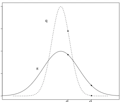
In the case of the MHIS the need of a proposal that mimics the target is very important. One useful strategy is to choose a proposal with mode, and curvature at the mode, matching these of the target distribution. Moreover, in order to be sure that the whole target is explored we want the proposal to have heavier tails than the target distribution; this is known as the heavy tail rule. If the proposal has lighter tails than the target then it is highly likely that the proposed values will be within the main body of the distribution and the tails will not be well explored. However, when eventually the chain does move to the tail, the probability that subsequent proposals will be accepted is very small and

so the chain mixes very poorly. For instance consider thatθ is one dimensional and the

proposal has lighter tails than the taregt as illustrated in Figure 2.1 and a relatively

constant ratio π(θ)/q(θ) for values of θ in the main body of the distribution. Assume

that the current value of θis θ1 and a move toθ2 is proposed. In this case, π(θ2)/q(θ2)

will be very high and inceπ(θ1)/q(θ1) is relatively constant, the value of the acceptance

ratio, in 2.1.11, π(θ2)q(θ1) π(θ1)q(θ2) = π(θ2)/q(θ2) π(θ1)/q(θ1) .

(42)

0.0 0.2 0.4 0.6 0.8 θ2 θ1 ● ● ● ● π q

Figure 2.1: Density of the proposal distribution, q(θ) (dashed line) and of the target

distributionπ(θ) (solid line).

will be large. Therefore, such a proposed value as θ2 will be accepted. If however we

consider the opposite scenario of currently being to θ2 and proposing a move to θ1,

the ratio π(θ1)/q(θ1) is almost constant and π(θ2)/q(θ2) is very high. Therefore, the

acceptace ratio

π(θ1)q(θ2)

π(θ2)q(θ1)

= π(θ1)/q(θ1)

π(θ2)/q(θ2)

will be very small and such moves will be always rejected making the return back to the main body of the target difficult .

As a final note we would like to mention the effect of choosing as a proposal the prior distribution. This might seem quite tempting since the acceptance ratio simplifies further to just the ratio of the likelihoods. However, if the likelihood is informative, so that the posterior and prior are dissimilar, then we might end up with very low acceptance rates. In particular, we will be proposing values that have high probability according to the

(43)

prior but may not correspond to a large likelihood value and having, as a result, to reject these moves. See Gamerman & Lopes (2006) for a detailed discussion.

2.1.8 Adaptive MCMC

As already mentioned, an appropriately shaped and also optimally tuned proposal distri-bution is crucial for constructing a well-mixing MCMC scheme. However, in complicated, high-dimensional targets this can be extremely difficult especially when a good estimate of the posterior covariance matrix is not available. But even in low-dimensional targets

defining an optimal value for the tuning parameter λ can be painful since, usually in

practice, this has to be done through trial an error.

Adaptive MCMC was created to provide a solution to such problems and minimise, as much as possible, the user intervention. The idea behind adaptive MCMC schemes is to use the information that becomes available as the sampler runs. This information is used in order to automatically update the variance of the proposal distribution, using estimates obtained from the empirical distribution of the chain so far, according to a pre-defined updating rule.

Although in practice such schemes have by now become straightforward to implement there are certain issues to be considered. First of all, if the chain starts away from the main body of the target distribution, i.e., in the tails, then there is a chance for the chain to stay there for a long time and, in the time available, not explore areas with high posterior probability. This is because the algorithm learns about this insignificant area and automatically adjusts the proposal distribution so that it can efficiently explore that specific part of the support. Therefore, even if the sampler is ergodic, given that it is run for a finite number of iterations, the posterior estimates obtained might not represent

(44)

the truth since it may take a long time to obtain an adequate sample. For that reason, in practice, the proposal distribution will sometimes use a mixture of an adaptive and a non-adaptive kernel in order to minimise the chance of being trapped in such areas (see for instance Sherlock et al. (2013) and Fearnhead et al. (2014)).

Another issue is by how much and how often should the proposal variance change during the MCMC scheme. For instance, it is sensible to initially let the sampler run with a fixed proposal and once a certain number of accepted moves has been achieved then start adapting the proposal distribution. This is to ensure that the chain has moved sufficiently so that the covariance matrix is not singular.

However, since the transition kernel keeps changing for as long as the sampler runs, convergence to the stationary distribution is not anymore guaranteed and hence nor is the ergodicity of the chain. There has been a lot of research on the ergodicity and convergence properties of adaptive MCMC schemes and two important concepts that have arisen are

the diminishing adaptation and the containment condition. Let (θn, γn) be the position

and transition kernel at then-th iteration under the adaptive scheme. Given the starting

value and initial kernel (θ0, γ0), the containment condition states that if the chain were

to start at θn with a non-adaptive fixed kernel γn then, irrespective of n, the chain

will have nearly converged to π(·) after N iterations, for large enough N. For nearly

all possible (θn, γn). As mentioned in Brooks et al. (2011), Chapter 4, the containment

condition will usually hold for most adaptive schemes given that a reasonable adaptation rule is used and therefore focus is placed on the notion of diminishing adaptation.

Diminishing adaptation suggests that changes in the proposal should become negligible as the chain evolves. This is to ensure that after a large number of iterations the successive transition kernels are similar and therefore reach an equilibrium. However, these changes

(45)

should also be large enough to reflect necessary changes in the covariance matrix.

For a thorough review and theoretical justifications on convergence and ergodicity results of adaptive MCMC we refer the reader to Andrieu & Thoms (2008) and Roberts & Rosenthal (2009) and the references therein.

2.2 Model based geostatistics

As mentioned in the Introduction of the thesis, Geostatistics concerns the study of a continuous spatial phenomenon. This phenomenon is usually modelled through a

sta-tionary Gaussian process,{S(x) :x∈_R2_}_{. By stationary we mean that the expectation}

and variance of the process is the same for allxand the correlation between S(xi) and

S(xj) only depends on the distance betweenxi andxj. Additionally, the Gaussianity of

the process S(x) implies that S(x1), ..., S(xd) are jointly normally distributed for any

set of locationsx1, ..., xd, . This process however, is not directly observed. Instead, there

is available only a finite sample of observations of a random variable, Y, at specific

sampling locations, xi, i = 1,2, ..., d, over the area of interest. These observations, y,

are usually assumed to be either identical to or a noisy version of the underlying true process or of a function of it. Interest usually lies in predicting the realisation of the process, or a functional of it, at unsampled locations or making inference about some parameters of the model.

The term ‘model-based geostastics’ was introduced in the seminal paper of Diggle et al. (1998) to describe the unified modelling and inferential framework provided by the au-thors.

(46)

spatial model and show how this is extended to the generalised linear spatial model just like the simple linear model extends to a GLM. The LSM and the GLSM can be viewed as a linear or generalised linear mixed-effects model (Breslow & Clayton 1993) respectively where the random effects form a Gaussian random field.

In Section 2.2.2 we outline the simple LSM along with the inferential procedure usually used. Section 2.2.3 presents the most widely used covariance functions used to model the spatial dependence and the characteristics that each one bestows on the underlying process. Finally, in Section 2.2.6 we describe the GLSM and review some of the current MCMC schemes used for inference in Section 2.2.7. Unless otherwise stated, the two main sources of information for this Section are Diggle et al. (2007) and Diggle et al. (2003).

2.2.1 The Gaussian process

As it constitutes a key component of the linear spatial model this section focuses on the definition of the Gaussian process and the notion of weak and strong stationarity.

Definition 2.2.1. A stochastic process, or random field, S with parameter space T is a collection of random variables{S(x) :x∈T}. The dimension ofT isN and the random variablesS(x)are vectors of dimension nthen the random fieldS is said to be an(N, n)

random field.

In our settingxrepresents the spatial coordinates of a sampling point and therefore the

setT is of dimensionN = 2. Also, at eachx,S(x) is one dimensional and therefore gives

rise to an (2,1) dimensional random field. For every stochastic process we can define the

mean and covariance function given by

(47)

respectively. If the mean function of the process S is constant for every x and the

covatriance function,c(xi,xj), only depends on the differencexi−xj, i.e.,

µ(x+t) =µ(x) and c(xi+h, xj+h) =c(xi, xj)

then the process S is said to be weakly stationary. A stronger form of statioanrity is

that of strong stationarity. The stochastic process S is said to be (strongly) stationary

if, its finite-dimensional distributions are invariant under the operation (+), i.e., if the

joint distribution of (S(x1+h), ..., S(xd+h)) is independent of hfor all xj ∈R2 and

anyd≥1.

Definition 2.2.2. The Gaussian process S, or a Gaussian random field, is a random field for which the joint distribution of (S(x1), ..., S(xd)) is multivariate Gaussian for

any finited≥1 and every (x1, ...,xd).

In the case of a Gaussian process weak stationarity implies strong stationarity. For that reason in the following sections we do not distinct the two and in general refer to a stationary Gaussian process without clarifying whether the process is weakly or strongly stationary. In general though this does not hold. If a stochastic process is strongly sta-tionary then it is also weakly stasta-tionary but the opposite does not hold. For a thorough study of Gaussian processes and in general random fields we refer the reader to Adler & Taylor (2007).

2.2.2 The linear spatial model (LSM)

Let {S(x) : x ∈ _R2_} _{be the underlying process of interest and} _y _{= (}_y

1, ..., yd)

0

be a

realisation of the observable random variable Y = (Y1, ..., Yd)

0

at sampling locations

(48)

explanatory variables measured at the sampling locations xi. In practice, S(xi), i =

1, ..., d, is assumed to be normally distributed with mean 0 and marginal variance σ2.

The correlation structure of the process S(x) will be discussed later. For i = 1, ..., d,

conditionally onS(x),Yiare assumed to be independent following a normal distribution

with varianceτ2and mean linearly related tof_iandS(xi). The equivalent mathematical

formulation of the model is given by,

Yi=f

0

iβ+S(xi) +Zi, i= 1, ..., d (2.2.1)

where Zi ∼ normal 0, τ2

and are mutually independent. At a specific location, even if the true value of the underlying process were known there would be some variability between consecutive measurements. Such variations are depicted by the conditional

vari-ance, τ2, of Yi|S(xi),β which is either interpreted as measurement error or small scale

variation.

It is intuitive to assume that nearby locations would give rise to similar measurements while the correlation between two locations fades away as their distance increases. The al-ternative, where the correlation increases with distance, would not lead to a positive

def-inite covariance matrix. Let S := (S(x1), ..., S(xd))

0

and Cor(S(xi), S(xj)) = ρ(uij;φ)

whereρ(·;φ) denotes a correlation function parametrised over some correlation

param-eterφ. Then it follows that,

S ∼MVN 0, σ2R(φ)

(2.2.2)

(49)

conse-quently

Y ∼MVN F β, σ2R(φ) +τ2I

(2.2.3)

with F representing the design matrix, with rows f0_i, and I being the d×d identity

matrix.

A widely used equivalent formulation considers an underlying Gaussian process which does not have a constant zero mean. In this case the covariate information is incorporated

in to the mean of the process. If we defineη:=F β+S, then,

Y =η+Z, (2.2.4) whereη= (η(x1), ..., η(xd))∼MVN F β, σ2R(φ) ,Z ∼normal 0, τ2I . Equivalently, Yi =f 0 iβ+S(xi) +Zi= ηi+Zi, for i= 1, ..., d (2.2.5)

where marginally, ηi ∼Normal f0iβ, σ2

. Note that the process {η(x) : x∈ R2} is no

longer stationary as defined in Section 2.2.1 but, as mentioned in Diggle et al. (2007), it

is covariance stationary. In the absence of explanatory variables, where f0_iβ is replaced

by a constant and fixed mean effectβ, then bothη(x) andS(x) are stationary Gaussian

processes.

Although the working framework of the normal model is well established, the assumption

of a linear relationship between the response variable Y and the signal process appears

to be quite unrealistic in real life phenomena. Consider for instance applications where

the observable variableY concerns counts or in general has an asymmetric distribution.

(50)

Gaussian data. Historically, before the introduction of GLSMs, approximate normality of the response variable was achieved through a transformation of the data and then inference was carried out under the Gaussian framework. A widely used family of such transformations is the Box-Cox (Box & Cox 1964) which however can be applied to strictly positive-valued data and comes at the additional cost of estimating an addi-tional parameter. Addiaddi-tionally, after such transformations, the model parameters, i.e.,

β, might not have a sensible natural interpretation. For a more detailed discussion and

implementation of Box-Cox transformations on the geostatistical model see Christensen, Diggle & Ribeiro (2001).

To simplify notation for the rest of this thesis we will suppressS(xi) to Si and η(xi) to

ηi.

2.2.3 Models for the correlation structure

In the previous section we briefly discussed some of the assumptions made regarding the correlation structure of the latent process. For instance, the process is often assumed to be stationary, isotropic and also the correlation between any two points should decrease as the distance increases. In addition, the correlation function used should be positive definite.

A flexible family of correlation functions satisfying these properties is the Mat´ern family

as introduced by Mat´ern (1960) given by,

ρ(u;φ, κ) = (u/φ)

κ_K

κ(u/φ)

2κ−1_Γ(_κ₎ , (2.2.6)

where Γ(·) is the Gamma function andKκ(·) corresponds to the modified Bessel function

(51)

correlation as the distanceuincreases. Given any two pointsu units apart, the largerφ

is, the higher the correlation between these two points will be.

The Mat´ern family gains its flexibility from the shape parameter κ since it defines the

differentiability of the correlation function at the origin or equivalently the smoothness

of the stochastic process S(·). In particular, κ reflects the short distance dependence of

the random field. Asκ increases the correlation remains at higher levels for longer and

the latent process becomes smoother.

A particular property that describes the smoothness of a stochastic process is the mean-square differentiability.

Definition 2.2.3. Mean Square Differentiability

A stochastic processS(x) with finite second moments is mean-square differentiable with mean-square derivativeS0(x) if as kk →0, E " S(x+)−S(x) kk −S 0 (x) 2# →0. (2.2.7)

Higher order derivatives can be obtained in a similar way. A very helpful result that pro-vides links between the differentiability of the correlation function at the origin with the mean-square differentiability of the stochastic process is the following. If the correlation

structure of the latent processS(x) is modelled using the Mat´ern family of correlation

of order κ then S(x) isdκ−1 times mean-square differentiable, where dκ denotes the

smallest integer that is not greater than κ. The more times mean-square differentiable

a process is the smoother it will be and therefore the stronger the correlation near the origin, i.e., for distances very close to 0.

(52)

of the Mat´ern family; the exponential and Gaussian correlation functions. In particular,

asκ→ ∞,ρ(u;φ)→exp{−(u/φ)2}corresponding to the Gaussian correlation function,

which should not be confused with the normal distribution, and forκ = 0.5 we obtain

the exponential correlation function given byρ(u;φ) = exp(−u/φ).

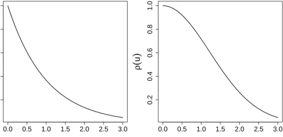
Figure 2.2 shows the exponential and Gaussian correlation functions. Since the

param-eters φ and κ are not orthogonal the values of φ have been matched so that in both

cases ρ(u) = 0.05 at the same distance u. For the exponential correlation φ = 1 and

for the Gaussian correlation function φ≈1.73. A process arising form the exponential

correlation function is not mean-square differentiable whereas process arising form the Gaussian correlation function is infinitely mean-square differentiable. As we see, in the case of the exponential correlation function the correlation drops quickly near the origin whereas in the case of the Gaussian the correlation stays near 1 for distances up to 0.5.

Other valid correlation functions outside the Mat´ern family, are the powered exponential

0.0 0.5 1.0 1.5 2.0 2.5 3.0 0.2 0.4 0.6 0.8 1.0 u ρ

(

u

)

0.0 0.5 1.0 1.5 2.0 2.5 3.0 0.2 0.4 0.6 0.8 1.0 u ρ

(

u

)

Figure 2.2: Correlation against distance. Left: exponential correlation function with

φ= 1, Right: Gaussian correlation function with φ= 1.73. The parameter φ has been

matched so that in both casesρ(u) = 0.05 at the same distance u.

(53)

by, ρ(u;φ, a) = exp − u φ a , 0< a≤2

embodies both the exponential, for a = 1, and the Gaussian correlation for a = 2.

However, the powered exponential family is not as flexible as the Mat´ern family since

the underlying processS(x) will not be mean-square differentiable for a <2.

The spherical correlation function,

ρ(u;φ) =        1−3 2 u φ+ 1 2 u φ 3 , 0≤u≤φ 0, u > φ,

is not mean-square differentiable but it is even more restrictive than the powered

expo-nential since it assumes that at distance equal toφthe correlation becomes exactly zero

and therefore has a finite range. As illustrated in Warnes & Ripley (1987), Mardia & Watkins (1989) and further discussed in Stein (1999), the spherical correlation function can usually give rise to a multimodal log-likelihood and therefore maximum likelihood techniques can be problematic when it comes to parameter estimation.

For simplicity, throughout this thesis we will usually denote the correlation matrix

R(φ, κ) simply by R. If we want though to stress that this matrix is a function of

φ, κwe will use R(φ, κ).

For a more thorough and technical investigation of correlation functions we refer the reader to Chapter 2 of Stein (1999).

For the LSM inference can be carried out both under the classical and Bayesian frame-work. The likelihood is tractable since the spatial process can be integrated out and maximum likelihood estimates of the parameters can be obtained. In a Bayesian setting