Dynamic chain graph models for time series network data

Open Research Online

The Open University’s repository of research publications

and other research outputs

Dynamic chain graph models for time series network

data

Journal Item

How to cite:

Anacleto, Osvaldo and Queen, Catriona (2017).

Dynamic chain graph models for time series network data.

Bayesian Analysis, 12(2) pp. 491–509.

For guidance on citations see FAQs.

c

2016 International Society for Bayesian Analysis

Version: Version of Record

Link(s) to article on publisher’s website:

http://dx.doi.org/doi:10.1214/16-BA1010

Copyright and Moral Rights for the articles on this site are retained by the individual authors and/or other copyright

owners. For more information on Open Research Online’s data policy on reuse of materials please consult the policies

page.

Dynamic Chain Graph Models for Time Series

Network Data

Osvaldo Anacleto∗ and Catriona Queen†

Abstract. This paper introduces a new class of Bayesian dynamic models for inference and forecasting in high-dimensional time series observed on networks. The new model, called the dynamic chain graph model, is suitable for multivariate time series which exhibit symmetries within subsets of series and a causal drive mechanism between these subsets. The model can accommodate high-dimensional, non-linear and non-normal time series and enables local and parallel computation by decomposing the multivariate problem into separate, simpler sub-problems of lower dimensions. The advantages of the new model are illustrated by forecasting traffic network flows and also modelling gene expression data from transcriptional networks.

Keywords:chain graph, multiregression dynamic model, network traffic flow forecasting, gene expression networks, network data, time series.

1

Introduction

Multivariate time series are often observed on a network or graph. Despite the ever-increasing research on network modelling, statistical dynamic modelling on networks has not been explored much so far (Kolaczyk,2009, Chapter 9). This paper proposes a new class of multivariate Bayesian dynamic models (West and Harrison,1997) for time series networks, called dynamic chain graph models.

Although Bayesian dynamic models have long been successfully applied in many different application areas (see, for example Velozo et al.,2014; Xiao et al.,2015; Nasci-mento et al.,2015; Quir´os et al.,2015), few of these models can accommodate complex high-dimensional series, while not being too demanding computationally. Furthermore, established Bayesian multivariate dynamic models such as the matrix normal dynamic linear model (Quintana and West, 1987) and its Gaussian graphical model extension (Carvalho and West, 2007) are only suitable for multivariate series whose component univariate series are similar and share a common structure.

The multiregression dynamic model (MDM) (Queen and Smith, 1993) is an alter-native model that does not require all the component univariate time series to have a common structure. This model assumes a conditional independence and causal struc-ture among time series components at each time step, as expressed by a directed acyclic graph (Lauritzen,1996). This graph is then used to decompose then-dimensional model into n separate conditional models, each of which is a univariate Bayesian dynamic model. As such, the MDM can accommodate arbitrarily high-dimensional structures, while enabling local and parallel computation.

∗_{The Roslin Institute and R(D)SVS, University of Edinburgh, UK,[email protected]} †_{Department of Mathematics and Statistics, The Open University, UK,[email protected]}

c

The MDM has been extensively used in a variety of applications: brand sales fore-casting (Queen, 1994), traffic flow forecasting (Queen et al.,2007; Queen and Albers,

2009; Anacleto et al., 2013a,b), functional magnetic resonance imaging (Costa et al.,

2015; Oates et al.,2015a,b), financial portfolio analysis (Zhao et al.,2015) and electric-ity demand forecasting (Zhao, 2015). However, the directed acyclic graph used in the MDM may be too restrictive: only directional associations between individual series can be accommodated, and no symmetric associations are allowed.

Queen and Smith (1992) developed a Bayesian dynamic model called the dynamic graphical model, in which a chain graph (Wermuth and Lauritzen, 1990) represents a multivariate time series Yt at each time t, with both directional and symmetric

associations between the individual time series. In that model, Yt is partitioned into

ordered chain components, which arecompleteundirected graphs and are connected by directed edges. However, if two chain components are connected in this model, then there must be a directed edge fromevery variable in the first chain component toevery

variable in the second. Also, the dynamic graphical model cannot accommodate chain components as sparse undirected graphs, which simplify estimation of the observation covariance matrix (Carvalho and West,2007; Prado and West,2010).

This paper presents a Bayesian dynamic model based on a chain graph which does not rely on the stringent assumptions required for the dynamic graphical model devel-oped in Queen and Smith (1992). This new model not only enables sparsity on chain components, but it also allows for unrestricted directed edges between them, thus ac-commodating more complex dependence patterns among multivariate time series com-ponents. It is shown that, like the MDM, computation in this new model is simplified and parallelizable since the multivariate problem is decomposed into separate, simpler sub-problems of lower dimensions, although, unlike the MDM, not all of these will be univariate.

The proposed model is illustrated using two application areas: road traffic flow fore-casting and gene expression modelling. Both applications are examples where the MDM cannot capture all types of dependencies among the time series components.

2

Basic graph theory concepts and notation

Before defining the new model in the next section, some notation and terminology is introduced. The terms network and graph are interchangeably used throughout this paper. A chain graph is defined as a pair (V, E), where V is a finite set of nodes(or

vertices) andE is a subset of ordered pairs of nodes, callededges.

Figure 1 shows an example of a chain graph for a 7-dimensional vector X with chain components{X1, X2}, {X3, X4}, {X5, X6} and{X7}. If there is a directed edge

from Xi toXj, thenXi is a parent ofXj while Xj is a child ofXi, and ifXk and Xl

are connected by an undirected edge, then they are neighbours. For set of variablesA, the parents, children and neighbours ofAare denoted, respectively, pa(A), ch(A) and ne(A). The boundary of setAis bd(A) = pa(A)∪ne(A). A path of lengthnfrom α

to β is any sequence (α0 =α, . . . , αn =β) of distinct nodes such that (αi−1, αi)∈ E

Xj is a descendant of Xi: the descendants of the set of variables Ais denoted de(A).

The non-descendants ofAare nd(A) =X\(de(A)∪A). Then, for eachXi,i= 1, . . . , n

(Lauritzen, 1996),

Xi⊥⊥{nd(Xi)\bd(Xi)} |bd(Xi). (1)

For example, in Figure 1, pa(X6) = {X3, X4}, ch(X6) = {X7}, ne(X6) = {X5},

de(X6) ={X7}, nd(X6) ={X1, X2, X3, X4, X5}and soX6⊥⊥{X1, X2)} | {X3, X4, X5}.

Figure 1: Example of a chain graph.

3

The dynamic chain graph model

Thedynamic chain graph model (DCGM) is defined for time series which can be rep-resented over time by a dynamic chain graph. The DCGM makes explicit use of the dynamic chain graph structure of the series to simplify computation. Before defining the DCGM in Section3.2, a dynamic chain graph representation for time series, together with the associated conditional independence relationships between the component time series, is presented in Section3.1.

Firstly, some notation is required. Let{Yt}t∈Nbe ann-dimensional time series and

suppose thatYtis partitioned intoN vector time series of dimensionsr1, . . . , rN with

N i=1ri = n, so that Y T t = (Yt(1)T, . . . ,Yt(N)T) where, for i = 1, . . . , N, Yt(i)T = (Yt1(i), . . . , Ytri(i)). LetY t = (Y1, . . . ,Yt)T,Yt(i) = (Y1(i), . . . ,Yt(i))T andYtj(i) =

(Y1j(i), . . . ,Ytj(i))T, and letyt,yt(i) and ytj(i) be the realizations of Yt,Yt(i) and

Ytj(i), respectively.

3.1

Representing multivariate time series with dynamic chain

graphs

The dependence structure of a dynamic chain graph can be divided into a set of intra time-slice dependencies, which represent associations among time series components in a fixed timet∈N, and a set ofinter time-slice dependencies, which represent associations among time series components across time.

Intra time-slice dependencies

Suppose that, at each timet∈N, there is an association structure between all individual time series within each vector series Yt(1), . . . ,Yt(N) so that, for each i = 1, . . . , N,

Yt1(i), . . . , Ytri(i) form an undirected chain component in a chain graph. Suppose also that for each timet ∈Nthere is a causal drive through the system and a conditional independence structure (which is the same structure for each time t ∈ N) so that Yt(1), . . . ,Yt(N) are ordered chain components in the chain graph with pa(Ytj(i))⊆

{Yt(1), . . . ,Yt(i−1)}. For example, consider the time seriesYtrepresented at timet

by the chain graph given in Figure 2. Here there are three chain components (so that

N = 3):{Yt1(1), Yt2(1)},{Yt1(2), Yt2(2), Yt3(2)}and{Yt1(3), Yt2(3)}, withr1= 2,r2= 3

and r3 = 2. Thus YTt = (Yt(1)T,Yt(2)T,Yt(3)T) where Yt(1) = (Yt1(1), Yt2(1))T,

Yt(2) = (Yt1(2), Yt2(2), Yt3(2))T andYt(3) = (Yt1(3), Yt2(3))T.

Inferring intra-time slice dependencies from data is an important research area. This problem is not the focus here, but it is briefly mentioned in Section6.

Figure 2: Example of intra-time slice dependencies in a chain graph representation of a 7-dimensional time series at timet.

Inter time-slice dependencies

The chain graphs defined above for the time series vectors Yt(1), . . . ,Yt(N) at each

t ∈ N can be linked together by assuming inter time-slice dependencies, so that a

dynamic chain graphfor the time series{Yt}t∈Nis obtained. For a time series up to time

t, represented by Yt(1), . . . ,Yt(N), the inter time-slice dependencies of a time series componentYtj(i),i= 1, . . . , N,j= 1, . . . , ri, are represented by its parents at previous

time steps, which are allowed to be from{Yk(1), . . . ,Yk(i)},k= 1, . . . , t−1. Together with the contemporaneous parents defined in the previous section, in a dynamic chain graph we then have

pa(Ytj(i))⊆ {Yt(1), . . . ,Yt(i−1),Yt−1(i)}. (2)

The parent set pa(Ytj(i)) is assumed to be the same at each time t∈N.

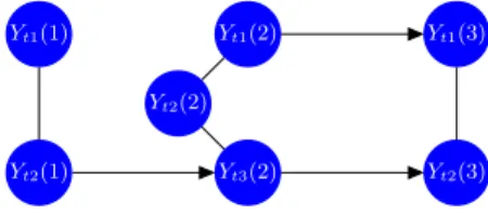
Figure3shows a dynamic chain graph example based on the chain graph of Figure2

and considering all time points up to timet. Notice that ifYtj(l) is a parent ofYtk(m),

it is not necessary thatYt_j−1(l) is also a parent ofYtk(m), nor thatYtj−1(l) is a parent

ofYtj(l).

Dynamic chain graph conditional independence structure

The dynamic chain graph defines a conditional independence structure among contem-poraneous variables as stated in the following theorem.

Figure 3: Example of a dynamic chain graph for the 7-dimensional time series with intra-time slice dependencies (black edges) defined in Figure2. Inter time-slice dependencies are represented by green edges. The figure shows inter time-slice dependences for the series at a arbitrary time such that these dependencies are the same for any time step

t >1. Undirected edges between processes represent intra-time slice relationships. For example, the undirected edge connectingYt₁−1(1) andYt₂−1(1) means that there is an undirected edge betweenYi1(1) andYi2(1) fori= 1, . . . , t−1.

Theorem 1. Let{Yt}t∈Nbe represented by a dynamic chain graph whereYtcan be

de-composed, for each timet∈N, into a set of ordered chain componentsYt(1), . . . ,Yt(N),

with such ordering remaining constant over time. Then, the following conditional inde-pendence statements hold for each time t∈N:

Yt(i)⊥⊥[{Yt(1), . . . ,Yt(i−1)} \pa(Yt(i))]|pa(Yt(i)). (3)

Proof. For notational convenience, define

Xt(i)T = (Yt(1), . . . ,Yt(i−1)), i= 2, . . . , N,

Zt(i)T = (Yt(i+ 1), . . . ,Yt(N)), i= 1, . . . , N−1,

where fori= 1,Xt(i) is∅, as isZt(i) fori=N.

For the dynamic chain graph representing Yt(1), . . . ,Yt(N) as described above, conditional independence statements (1) imply that for each t ∈ N, i = 1, . . . , N and

j= 1, . . . , ri,

Ytj(i)⊥⊥{nd(Ytj(i))\bd(Ytj(i))} |bd(Ytj(i)). (4)

Now, the set nd(Ytj(i)) consists of {Yt(i)\Ytj(i)} together with Xt(i), Yt−1(i) and

Zt−1(i), while bd(Ytj(i)) = pa(Ytj(i))∪ne(Ytj(i)), where pa(Ytj(i))⊆

Xt(i),Yt−1(i) from (2), and ne(Ytj(i))⊆ {Yt(i)\Ytj(i)}. Therefore, statement (4) becomes

Ytj(i)⊥⊥ Xt(i),{Yt(i)\Ytj(i)},Zt−1(i) \bd(Ytj(i)) |bd(Ytj(i))

In particular, this means that

Ytj(i)⊥⊥[{Yt(1), . . . ,Yt(i−1)} \bd(Ytj(i))]|bd(Ytj(i)).

But since ne(Ytj(i)) ⊆ {Yt(i)\Ytj(i)} for each j = 1, . . . , ri, then collectively

bd(Yt(i))≡pa(Yt(i)), so that the conditional independence statements in (3) hold.

As will be seen later, Theorem 1 is important for the proposed model as it plays a key role in breaking the multivariate problem intoN smaller subproblems. Next the new model will be defined.

3.2

Model definition

For time series{Yt}t∈Nrepresented by a dynamic chain graph as described above, the

DCGM is defined for all t ∈Nas follows. The initial information available is denoted byD0. Observation equations: Yt(i) =Ft(i)Tθt(i) +vt(i), vt(i)∼(0,Σt(i)), (5) i= 1, . . . , N, System equation: θt=Gtθt−1+wt, wt∼(0,Wt), (6) Initial information: θ0|D0∼(m0,C0). (7) HereFt(i)T= (Ft1(i)T, . . . ,Ftri(i) T_{), wheres} j-dimensional vectorFtj(i),j= 1, . . . , ri,

is allowed to be an arbitrary, but known, function of the contemporaneous values of pa(ytj(i)) and yt−1(1), . . . ,yt−1(i), but not yt(i + 1), . . . ,yt(N) or yt(i). The

vec-tor θT

t = (θt(1)T, . . . ,θt(N)T) is a s-dimensional state vector, where θt(i) is the si

-dimensional state vector for Yt(i) with si =

ri

j=1sj and s =

N

i=1si. The ri×ri

matrixΣt(i) is the observation covariance matrix forYt(i). The s×smatrices Gt=

blockdiag(Gt(1), . . . ,Gt(N)) and Wt = blockdiag(Wt(1), . . . ,Wt(N)), where Gt(i)

andWt(i) are, respectively, thesi×sistate evolution matrix and state evolution

covari-ance matrix forθt(i),i= 1, . . . , N, are allowed to be functions ofyt−1(1), . . . ,yt−1(i),

but not yt−1_{(i + 1), . . . ,y}t−1_{(N). In the s-dimensional vector w}T

t = (wt(1)T, . . . ,

wt(N)T),wt(i) is the si-dimensional system error vector for θt(i), i= 1, . . . , N. The

s-dimensional vectorm0ands×smatrixC0= blockdiag(C0(1), . . . ,C0(N)) are

mo-ments ofθ0|D0. Errorsvt(1), . . . ,vt(N) andwt(1), . . . ,wt(N) are mutually

indepen-dent of each other and through time.

To illustrate the DCGM, consider once again the time series represented by the dynamic chain graph in Figure 3. Separate observation equations (5) are specified for Yt(1), Yt(2) andYt(3): Ft(1)T= (Ft1(1)T,Ft2(1)T), such that Ft1(1)Tis a function

of yt₁−1(1); Ft(2)T = (Ft1(2)T,Ft2(2)T,Ft3(2)T), such that Ft1(2)T is a function of

yt₁−1(1) andFt3(2)T is a function ofyt3−1(2) andyt2(1);Ft(3)T= (Ft1(3)T,Ft2(3)T),

such that Ft1(3)T is a function of y1t−1(3) and yt1(2) and Ft2(3)T is a function of

yt₂−1(3) and y_t3(2). Additionally, Ft(1)T, Ft(2)T and Ft(3)T can also be functions of

Corollary1to follow presents a key result for the DCGM. Corollary1follows on from a theorem which is provided in the Supplementary Material for the paper (Anacleto and Queen,2016). The proofs of this theorem and of the corollary are also provided in the Supplementary Material.

Corollary 1. If⊥⊥N_i=1θ0(i), then under the DCGM, for allt∈N, 1. ⊥⊥N_i=1θt(i)|yt, and

2. θt(i)⊥⊥yt(i+ 1), . . . ,yt(N)|yt(1), . . . ,yt(i), for i= 1, . . . , N−1.

Corollary1 means that ifθt(1), . . . ,θt(N) start independent, then they remain so

after sampling: initial independence is ensured sinceC0 is block diagonal in (7).

Corol-lary 1and Theorem1 together mean that each parameter vectorθt(i) can be updated

separately within the conditional multivariate model for Yt(i) |pa(yt(i)), and

condi-tional forecasts for Yt(i) | pa(yt(i)) can be found separately, since the joint forecast

distribution can be expressed as

f(y_t|yt−1) = N i=1 θt(i) f(y_t(i)|pa(y_t(i)),θt(i))f(θt(i)|xt−1(i),yt−1(i))dθt(i).

Another consequence of θt(1), . . . ,θt(N) remaining independent after sampling, is

that the smoothing distributions θt−k(i)| yt,k = 1, . . . , t−1, can be calculated

sep-arately for each i = 1, . . . N. (For example, when normal errors are assumed, each smoothing density has the form as given in West and Harrison, 1997, page 113). The DCGM therefore decomposes then-dimensional model intoNseparate conditional mul-tivariate models of smaller dimensions. This decomposition greatly simplifies model computations, breaking what can be a highly complex multivariate problem into more manageable parts.

It is worth emphasizing that the regression vectors, Ftj(i), i = 1, . . . , N, j =

1, . . . , ri, are functions of the contemporaneous values of the parents of Ytj(i), which

are unknown at timet−1 when forecasts forYtj(i) are required. Although the

regres-sion vector at timetis usually known before timetin the Bayesian dynamic linear model (DLM) framework, the idea of having unknown random variables in the regression vec-tor is not new: both the MDM and Queen and Smith (1992) dynamic graphical model also allow the regression vectors to be functions of the (unknown) contemporaneous values of parents, while Wang et al. (2011) also consider DLMs with random vectors. To obtain forecasts forYt(1), . . . ,Yt(N) in the DCGM, marginal forecasts

(marginal-izing over pa(y_t(i))) are required. Although the marginal distributions are not generally simple distributional forms, it is usually straightforward to calculate the marginal fore-cast moments from the conditional ones using the identities E(X) =E[E(X |Z)] and

V(X) =E[V(X |Z)] +V[E(X|Z)].

The MDM is a special case of the DCGM in which all the chain components are single values so that N = n. In both models, the set of contemporaneous variables

pa(ytj(i)) are used as regressors when modelling Ytj(i) and both models break the

multivariate problem into simpler sub-problems. However, whereas the MDM breaks the n-dimensional problem into n univariate ones, the dynamic chain graph model breaks the problem intoN separate multivariate models for the chain components.

In this respect the proposed model is like the dynamic graphical model of Queen and Smith (1992). The DCGM is, however, far more general: ifYtk(l) is a parent ofYtj(i)

in a chain graph representingYt, then the dynamic graphical model would requireall

components of the vector Yt(l) to be parents to all components of the vector Yt(i),

whereas in the DCGMYtj(i) can have any number and combination of component series

of Yt(1), . . . ,Yt(i−1) as parents and the other components ofYt(i) need not have

the same parents. Also, in the dynamic graphical model, all component series within a chain component must be pairwise connected, whereas this need not be the case in the DCGM. Further, unlike the dynamic graphical model, no distributional assumptions are made for the priors or error distributions in the DCGM,Ft(i) in (5) need not be a

linear function of its parents, and no assumptions are made regarding the multivariate dynamic models for Yt(1), . . . ,Yt(N).

The dynamic graphical model uses matrix normal DLMs (Quintana and West,1987) to model each ofYt(1), . . . ,Yt(N). This model is conjugate and thus computationally

simple and quick to use. However, although the matrix normal DLM can be used to model Yt(1) in the DCGM, it is not appropriate for Yt(i)| pa(yt(i)), i = 2, . . . , N:

the matrix normal DLM would require each of the individual series Yt1(i), . . . , Ytri(i),

i= 2, . . . , N, to have thesameregression vector so thatFt1(i) =· · ·=Ftri(i), whereas in the DCGM eachFtj(i),j= 1, . . . , ri, is potentially different because it is a function

of pa(ytj(i)), and pa(ytj(i)) is not necessarily equal to pa(ytk(i)), forj=k.

The simplest models for Yt(1), . . . ,Yt(N) are DLMs where Ftj(i), j = 1, . . . , ri,

i= 1, . . . , N, is a linear function of regressor(s) pa(ytj(i)) and all distributions in (5)–

(7) are normal. This is thelinear dynamic chain graph model (LDCGM). In the next section, the LDCGM is applied to forecast road traffic network flows.

4

Application: forecasting traffic network flows

Anacleto et al. (2013a,b) used a linear version of the MDM, the LMDM, to forecast flows in a road traffic network at the intersection of three busy motorways near Manchester, UK. Figure 4(a) shows a schematic diagram of the network: arrows represented by the roadways indicate the direction of travel and circles denote the flow data collection sites which are labelled by identification numbers. In this paper, an LDCGM is used to forecast flows in part of this network and the performance of the LDCGM and the LMDM is compared.

Time series data of 5-minute counts of vehicles passing over induction loops (see Li, 2009) in the Manchester network for November and December 2010 are available from the Highways Agency in England (http://www.highways.gov.uk/). Let Yt(k)

denote the traffic flow (5-minute vehicle counts) at site k at time t. Anacleto et al. (2013b) elicited a directed acyclic graph (DAG) to represent these traffic flow series.

Figure 4: (a) Schematic diagram of a traffic network near Manchester. (b) A chain graph for a subset of data collection sites of the Manchester network.

In that DAG, all variables have one or two parents except for the time series at the four entrances to the network, namelyYt(9206B),Yt(6013B),Yt(9188A) andYt(1431A),

which do not have parents: these variables without parents are referred to as root nodes. Queen et al. (2008) showed that, for any two root nodes Yt(k) and Yt(l) being

modelled by an LMDM, the forecast covariance between Yt(k) and Yt(l) is 0. This

result also holds for the general MDM. However, this is an unrealistic assumption for the Manchester network traffic flow series, where the root nodes (the series at the entrances to the network) can be highly correlated (Anacleto, 2012). In this case, a chain graph representing the root nodes in a chain component may be a more suitable representation of the flow series.

For clarity of presentation, consider a small subset of the Manchester network com-prising the flow series at the entrances to the network and four of the adjacent down-stream flows (the four root nodes with one of each of their respective children in the DAG representation). For notational convenience, let

Yt(9206B) =Yt1(1), Yt(6013B) =Yt2(1), Yt(9188A) =Yt3(1), Yt(1431A) =Yt4(1),

Yt(9200B) =Yt(2), Yt(6007L) =Yt(3), Yt(9193J) =Yt(4), Yt(1437A) =Yt(5),

and set Yt= (Yt(1)T, Yt(2), . . . , Yt(5))T whereYt(1)T = (Yt1(1), . . . , Yt4(1)). A chain

graph representation ofYtis given in Figure4(b): directed edges fromYtj(1) toYt(j+1),

j = 1, . . . ,4, represent parent child relationships from the original DAG representation in Anacleto et al. (2013b), and undirected edges represent associations between pairs of root nodes.

4.1

An LDCGM for the traffic network

The chain graph in Figure4(b) has only one multivariate chain component,Yt(1), while

the other chain components are single series. In this case an LDCGM can be defined in which a matrix normal DLM is used to model Yt(1), while conditional univariate

DLMs are used to modelYt(2), . . . , Yt(5).

A matrix normal DLM forYt(1) is specified in terms ofrowvectorYt(1)Tands1×4 matrix parameterΘt(1) = (θt1(1), . . . ,θt4(1)), whereθtj(1) is thes1-dimensional state

vector for Ytj(1), j = 1, . . . ,4. Yt1(1), . . . , Yt4(1) each has the same regression vector

Ft(1), and each state vector θt1(1), . . . ,θt4(1) has the same dimension (s1) and the

same state evolution matrix Gt(1).

DenotingθT_t = (θt(2)T, . . . ,θt(5)T), an LDCGM forYtin the Manchester network

is defined as follows for timest∈N.

Observation equations: Yt(1)T=Ft(1)TΘt(1) +vt(1)T, vt(1)∼N(0,Σt(1)), (8) Yt(i) =Ft(i)Tθt(i) +vt(i), vt(i)∼N(0, Vt(i)), i= 2, . . . ,5. (9) System equations: Θt(1) =Gt(1)Θt−1(1) +Ωt(1),Ωt(1)∼N(0,Wt(1),Σt(1)), (10) θt=Gtθt−1+wt,wt∼N(0,Wt). (11) Initial information: Θ0(1)|D0∼N(m0,C0(1),Σ0(1)), (12) θ0|D0∼N(m0,C0). (13)

Thes1-dimensional vectorFt(1) may be a function ofyt−1(1) but notyt(2), . . . ,yt(5);

si-dimensional vector Ft(i) is a linear function of pa(yt(i)), i = 2, . . . ,5; 4×4

ma-trixΣt(1) defines a cross-sectional covariance structure acrossYt(1);Vt(i) is the scalar

observation variance for Yt(i), i = 2, . . . ,5; Gt(1) is the s1×s1 state evolution

ma-trix for Θt(1); Gt = blockdiag(Gt(2), . . . ,Gt(5)) is the state evolution matrix for θt;

Ωt(1) is the s1 ×4 matrix of system errors for Θt(1) with matrix normal

distribu-tion (Dawid, 1981), with s1×4 mean matrix of zeros, s1×s1 left covariance matrix

Wt(1) and 4×4 right covariance matrixΣt(1); wt is the system error vector forθt;

Wt = blockdiag(Wt(2), . . . ,Wt(5)) is the state evolution covariance matrix for θt;

Θ0(1)|D0 has a matrix normal distribution withs1×4 mean matrixm0,s1×s1left

covariance matrixC0(1) and 4×4 right covariance matrixΣ0(1); and m0 andC0 are

the moments of θ0|D0. All model errors are mutually independent of each other and

independent through time.

Matrix Σt(1) and variances Vt(i), i = 2, . . . ,5, are estimated sequentially on-line

using conjugate inverse Wishart and gamma priors, respectively: see West and Harrison (1997, pages 108–112, 603–604). Conjugacy allows quick and easy computation.

To evaluate the effect of the joint modelling of Yt1(1), . . . , Yt4(1) in a chain

association structure. The graph for this LMDM is the DAG obtained by removing the undirected edges from the chain graph in Figure 4(b), so that Yt1(1), . . . , Yt4(1) are

unconnected root nodes and Ytj(1) is a parent ofYt(j+ 1), forj= 1, . . . ,4.

Series Yt(2), . . . , Yt(5) are modelled in exactly the same way via (9), (11) and (13)

in both the LMDM and the LDCGM, whereas in the LMDM each Ytj(1),j = 1, . . . ,4,

is modelled by a separate DLM of the form:

Obs. equation: Ytj(1) =Ftj(1)Tθtj(1) +vtj(1), vtj(1)∼N(0, Vtj(1)) (14)

Sys. equation: θtj(1) =Gtj(1)θt−1,j(1) +wtj(1), wtj(1)∼N(0,Wtj(1)) (15)

Initial info.: θ0j(1)|D0∼N(m0j(1),C0j(1)). (16)

Following Anacleto et al. (2013b), because of differences in flow patterns for different weekdays, for clarity of presentation only flows from Wednesdays are used here. In the absence of expert information, data from November were used to elicit all priors, while one-step ahead forecasts are obtained for December. Heavy snow caused several periods of disruption to the network traffic during December 2010. The models are thus compared when an explicit factor was affecting the traffic flows: it is at such times when forecasting is of most use for traffic control.

Traffic flow series exhibit daily patterns which both models need to accommodate. Following Anacleto et al. (2013a), cubic splines can model these daily patterns so that the regression vectors Ft(1) in (8) and Ft1(1), . . . ,Ft4(1) in (14) contain fixed basis

functions, whileΘt(1) in (8) andθt1(1), . . . ,θt4(1) in (14) contain dynamically evolving

spline parameters for individual series which are estimated sequentially online. In the matrix normal DLM, the sameFt(1), and hence basis functions, are used for each series

Yt1(1), . . . , Yt4(1). The daily patterns exhibited by Yt1(1), . . . , Yt4(1) are similar, and

variation in patterns is accommodated through each series having different parameters. Evolution matrices,Gt(1) in (10) andGt1(1), . . . ,Gt4(1), in (15) are identity matrices.

For both the LMDM and the LDCGM,Yt(2), . . . , Yt(5) are modelled in the same way:

separate regression DLMs are defined forYt(2), . . . , Yt(5) where eachYt(i),i= 2, . . . ,5,

has pa(yt(i)) =yt,i−1(1) as a linear regressor. The parameters for these regressors

ex-hibit daily patterns, and, following Anacleto et al. (2013a), these can also be modelled by cubic splines so thatFt(i) andθt(i) in (9) contain fixed basis functions and

dynami-cally evolving spline parameters, respectively. MatrixG˜t(i) in (11) is an identity matrix.

Exogenous variables — namely, speed, occupancy and headway — are available at each traffic site, and are also considered in the DLMs for Yt(2), . . . , Yt(5) using splines: see

Anacleto et al. (2013a) for details.

In the LDCGM, however, the matrix normal DLM for Yt(1) requires Yt1(1), . . .,

Yt4(1) to have the same regression vector Ft(1). Thus, it is not possible for Ytj(1)’s

model to include exogenous variables (i.e. speed, occupancy and headway) at that site as predictors, without also including exogenous variables at all the other sites inYt(1)

as predictors as well. Thus these predictors are not included forYt(1), and for fairness,

are also not included when modelling Yt1(1), . . . , Yt4(1) as root nodes in the LMDM.

As an alternative, predictors in Yt(1) could be included by using the seemingly

estimation. However, since the emphasis here is the evaluation of the effect of captur-ing both directed and undirected relationships with the LDCGM in comparison to just capturing directed relationships with the LMDM, a simpler model, such as the matrix normal DLM, can be used.

For both models, the observation variancesVt(2), . . . , Vt(5) in (9) are estimated

on-line following variance laws (West and Harrison,1997, Chapter 10.7) which relate the observation variance with mean flow, introduced in Anacleto et al. (2013b) to account for heterogeneity in traffic flow series. The cross-sectional covariance matrix, Σt(1), is

also estimated online. However, covariances betweenYt1(1), . . . , Yt4(1) don’t necessarily

change with the mean, so this matrix is estimated using the discounting variance learn-ing techniques of West and Harrison (1997, page 608) alone. For fairness of comparison variance laws are not used to model each Vtj(1) in equation (14), so that the scalar

observational variances ofYt1(1), . . . , Yt4(1) in the LMDM are also modelled using

dis-counting techniques only. Discount factors for all observation variances andΣt(1) vary

around 0.90. Prado and West (2010) point out that variance learning via discount fac-tors is only suitable when the (co)variances have a smooth and gradual random change. This is a reasonable assumption between 15:00 to 19:59 for these data, but not at other times. Thus only data between 15:00 and 19:59 are considered here.

Discount factors for all evolution covariance matrices in the LMDM and the LDCGM vary around 0.97, estimated on-line using standard discounting techniques (see West and Harrison, 1997, page 193). All discount factors are chosen by comparing the forecast accuracy of different models for each chain component, obtained through combination of observation and evolution discount factor values ranging from 0.80 to 1.

4.2

Forecast performance

Because of the heteroscedasticity of traffic flow series, the joint log-predictive likelihood (LPL), which assesses the precision of forecasts as well as point forecasts, is used when evaluating model forecast performance. The LPL calculates the log of the joint one-step ahead forecast distribution forYtbefore ytis observed, and then evaluates this at the

observed value y_t. The LPL is the aggregate of all these values over all time points. Anacleto et al. (2013a) provides details of the LPL for the LMDM and this is easily adapted for the LDCGM.

Table1shows the LPL values when forecasting Wednesday traffic flows in December 2010 using the LMDM and the LDCGM. The first row of Table 1 shows the forecast performance when only the four series inYt(1) are modelled: clearly the matrix normal

DLM for Yt(1) used in the LDCGM provides better forecasts than the independent

DLMs assumed for Yt(1) under the LMDM. From the second row of Table 1, the

LDCGM also performs better than the LMDM when all eight series are considered. The one-step ahead forecast means are very similar for both models, while the fore-cast variances for the LDCGM are slightly smaller, and so slightly more informative, than those for the LMDM. However, the real advantage of using the LDCGM is seen when considering multivariate forecasts. Figure 5shows (yt1(1), yt2(1)), represented by

LPL

Series considered LMDM LDCGM Yt(1) only −6,728 −6,154

Yt(1), . . . , Yt(5) −11,488 −10,914

Table 1: LPL values for the LMDM and the LDCGM.

for the LMDM and the LDCGM are represented by black and grey ellipses, respec-tively. In each plot, the forecast regions are smaller, thus more informative, for the LDCGM. The LDCGM forecast regions also clearly indicate a positive correlation be-tween (Yt1(1), Yt2(1)), which the other model does not. Forecast regions show positive

correlations amongst root nodes at other times too (Anacleto,2012).

In Figure5 the observed flows are not close to the centre of the forecast regions for either model. This could be due to variability in traffic flows which is not captured by the models. Neither model uses the exogenous variables speed, occupancy and headway, which may have captured some of this variability. The LDCGM does, however, perform better in Figure 5than the LMDM: for example, in Figure 5(b), the observed flow lies within the forecast region for the former, but does not for the latter.

Figure 5: Observed flows (·) and bivariate forecast limits at a pair of root nodes. The matrix normal DLM is not ideal for modelling Yt(1): the covariances vary

too much between times 20:00 and 14:59 to estimate Σt(1) through variance learning

discounting, and the exogenous variables speed, occupancy and headway, cannot be used. However, even with these restrictions, it has been shown that an LDCGM is worth consideration as an alternative to the LMDM for modelling traffic flows.

5

Application: modelling time series gene expression

data

The graph in Figure4(b) was elicited by exploiting the direction of traffic in the network as the causal driving mechanism across the time series. Alternatively, graphs can be also

inferred from data. As an example from biology, gene expression information, obtained through measurements of DNA transcription, can be used to infer networks describing regulatory mechanisms among genes (Kolaczyk, 2009). These networks can validate known gene associations and also allow the discovery of new gene relationships.

To capture the dynamics of biological processes, time-varying expression data may be preferable to transcriptional measurements obtained at steady-state. Dynamic Bayesian networks (DBNs) have been extensively applied to analyse time series gene expression data, as these models can capture feedback mechanisms which are ubiquitous in gene regulation (L`ebre,2009; Husmeier et al.,2011). Feedback mechanisms are captured in DBNs by replicating a DAG at each time-slice, with arrows connecting these DAGs based on the causal flow of time.

DCGMs can directly address two current limitations with DBNs for time series gene expression data. Firstly, DBNs usually assume that parents of a expression time series of a gene at a given time only take values at the previous time points. However, it is experimentally challenging to define a suitable sampling rate to collect time-varying transcriptional data so that this assumption is valid (Bar-Joseph et al.,2012). Secondly, even though symmetric associations between expression of different genes are common in transcriptional networks (Cantone et al., 2009), current DBNs for gene expression data cannot capture both directed and undirected edges in a graph.

The DCGM was used to model two gene expression datasets. The first dataset was obtained from an experiment involving the plant Arabidopsis Thaliana, as described in Smith et al. (2004). The expression of 800 genes at 11 different time points were measured and, following the correlation analysis in Opgen-Rhein and Strimmer (2007), 92 genes with the most significant connections were considered. The second dataset consists of gene expression measurements at 18 time points from an experiment aimed at understanding the developmental process of the mammary gland in mice (Stein et al.,

2004). For the second dataset, the focus is on 30 genes identified using cluster analysis by Abegaz and Wit (2013) as providing the best separation between developmental stages. Section S2 of the Supplementary Material provides a full description of the DCGM application to both datasets. The results of the application strongly suggest that the DCGM can improve modelling of gene expression data.

6

Final remarks

This paper presents a novel Bayesian dynamic model — the DCGM — for multivariate time series which assume a chain graph representation of the conditional independence structure among time series components. The new model deals with high-dimensional time series bydecouplingmultivariate time series of lower dimensions for sequential infer-ence, which can then berecoupledfor forecasting and decision analysis. This decoupling of high dimensional time series for sequential inference and recoupling for forecasting and decision making is also at the heart of the MDM and a model recently developed by Gruber and West (2015), although for these models the decoupling involves the uni-variate time series components, rather than subsets of multiuni-variate series. Under the DCGM, state parameters of the time series subsets remain independent after sampling,

which allows sequential and parallel inference of these subsets. The paper demonstrates how the DCGM improves time series modelling when there is evidence that conditional independence among time series components are better represented by both directed and undirected relationships in a graph, rather than directed relationships alone.

Application of the DCGM was illustrated here using traffic flow and gene expression networks. The model does, however, have much wider applicability to any multivariate time series which exhibits symmetric associations between groups of series together with a conditional independence and causal structure. The DCGM can also be used for any chain graph application (such as can be found, for example, in Cox and Wermuth,

1996) which may be part of a longitudinal study over time. What’s more, the fact that the model is very general and does not specify a particular multivariate model to use for each chain component, nor impose linearity and normality, increases its potential application areas.

The traffic flow time series analysed in this paper were obtained on a set of sites distributed over space, and so can be viewed as being generated from a spatio-temporal process. Multivariate time series from such processes are available in a variety of areas, and Cressie and Wikle (2011, Chapter 2.4) suggest that chain graphs are a natural tem-plate for representing such data. The DCGM could therefore be a potential candidate when modelling time series originating from spatio-temporal processes.

Whereas inference of DAGs and undirected graphs from data is a lively research area (see, for example, Scutari, 2013; Mohammadi and Wit,2015; Wang,2015), models for inferring chain graphs from data has received little attention (McCarter and Kim,2014). A structural learning method for chain graphs using time series data has been recently proposed by Abegaz and Wit (2013). However, their model is based on vector autore-gressive (VAR) processes, therefore relying on stringent assumptions of those models. In this context, following recent successful developments of DAG inference methods using the MDM (see Costa et al., 2015; Oates et al., 2015a,b), the DCGM is an important building block for inferring chain graphs from time series data.

Supplementary Material

Supplementary material for paper: Dynamic chain graph models for time series network data (DOI: 10.1214/16-BA1010SUPP; .pdf). Supplementary material available online includes the theorem for which Corollary 1 is a consequence, together with the proofs of that theorem and Corollary 1. It also includes the description and results of the application of the DCGM to two gene expression datasets, as mentioned in Section 5.

References

Abegaz, F. and Wit, E. (2013). “Sparse time series chain graphical models for recon-structing genetic networks.”Biostatistics, 14(3): 586–599. 504, 505

Anacleto, O. (2012). “Bayesian dynamic graphical models for high-dimensional flow forecasting in road traffic networks.” Ph.D. thesis, The Open University. 499,503

Anacleto, O. and Queen, C. (2016). “Supplementary material for paper: Dy-namic chain graph models for time series network data.” Bayesian Analysis. doi:http://dx.doi.org/10.1214/16-BA1010SUPP. 497

Anacleto, O., Queen, C., and Albers, C. J. (2013a). “Forecasting multivariate road traffic flows using Bayesian dynamic graphical models, splines and other traffic vari-ables.” Australian & New Zealand Journal of Statistics, 55(2): 69–86. MR3079021. doi:http://dx.doi.org/10.1111/anzs.12026. 492,498,501,502

Anacleto, O., Queen, C., and Albers, C. J. (2013b). “Multivariate forecasting of road traffic flows in the presence of heteroscedasticity and measurement errors.” Jour-nal of the Royal Statistical Society: Series C (Applied Statistics), 62(2): 251–270.

MR3045876. doi:http://dx.doi.org/10.1111/j.1467-9876.2012.01059.x. 492,

498,499,501,502

Bar-Joseph, Z., Gitter, A., and Simon, I. (2012). “Studying and modelling dynamic biological processes using time-series gene expression data.”Nature Reviews Genetics, 13(8): 552–564. 504

Cantone, I., Marucci, L., Iorio, F., Ricci, M. A., Belcastro, V., Bansal, M., Santini, S., Di Bernardo, M., Di Bernardo, D., and Cosma, M. P. (2009). “A yeast synthetic network for in vivo assessment of reverse-engineering and modeling approaches.”Cell, 137(1): 172–181. 504

Carvalho, C. M. and West, M. (2007). “Dynamic matrix-variate graphical models.”

Bayesian Analysis, 2(1): 69–97. MR2289924. doi: http://dx.doi.org/10.1214/07-BA204. 491,492

Costa, L., Smith, J., Nichols, T., Cussens, J., Duff, E. P., and Makin, T. R. (2015). “Searching multiregression dynamic models of resting-state fMRI networks using integer programming.” Bayesian Analysis, 10(2): 441–478. MR3420889. doi:http://dx.doi.org/10.1214/14-BA913. 492, 505

Cox, D. R. and Wermuth, N. (1996).Multivariate Dependencies: Models, Analysis and Interpretation, volume 67. CRC Press.MR1456990. 505

Cressie, N. and Wikle, C. K. (2011). Statistics for Spatio-Temporal Data. John Wiley & Sons.MR2848400. 505

Dawid, A. P. (1981). “Some matrix-variate distribution theory: notational consid-erations and a Bayesian application.” Biometrika, 68(1): 265–274. MR0614963. doi:http://dx.doi.org/10.1093/biomet/68.1.265. 500

Gruber, L. F. and West, M. (2015). “GPU-accelerated Bayesian learning in simultaneous graphical dynamic linear models.” Bayesian Analysis, 11(1): 125–149. MR3447094. doi:http://dx.doi.org/10.1214/15-BA946. 504

Husmeier, D., Werhli, A. V., and Grzegorczyk, M. (2011). “Advanced Applications of Bayesian Networks in Systems Biology.” In Stumpf, M. P. H., Balding, D. J., and Girolami, M. (eds.),Handbook of Statistical Systems Biology, 270–289. Wiley Online Library. MR2920207. doi:http://dx.doi.org/10.1002/9781119970606. 504

Kolaczyk, E. D. (2009). Statistical Analysis of Network Data: Methods and Models. Springer, New York. MR2724362. doi: http://dx.doi.org/10.1007/978-0-387-88146-1. 491,504

Lauritzen, S. L. (1996).Graphical Models. Oxford University Press.MR1419991. 491,

493

L`ebre, S. (2009). “Inferring dynamic genetic networks with low order independencies.”

Statistical Applications in Genetics and Molecular Biology, 8(1): 1–38. MR2476387. doi:http://dx.doi.org/10.2202/1544-6115.1294. 504

Li, B. (2009). “A non-Gaussian Kalman filter with application to the estimation of vehic-ular speed.”Technometrics, 51(2): 162–172. MR2668171. doi:http://dx.doi.org/ 10.1198/TECH.2009.0017. 498

McCarter, C. and Kim, S. (2014). “On Sparse Gaussian Chain Graph Models.” In

Advances in Neural Information Processing Systems, 3212–3220. 505

Mohammadi, A. and Wit, E. C. (2015). “Bayesian structure learning in sparse Gaussian graphical models.” Bayesian Analysis, 10(1): 109–138. MR3420899. doi:http://dx.doi.org/10.1214/14-BA889. 505

Nascimento, F. F., Gamerman, D., and Lopes, H. F. (2015). “Time-varying extreme pattern with dynamic models.” TEST, 1–19. 491

Oates, C., Smith, J., Mukherjee, S., and Cussens, J. (2015a). “Exact estimation of mul-tiple directed acyclic graphs.”Statistics and Computing, 1–15.http://dx.doi.org/ 10.1007/s11222-015-9570-9 492,505

Oates, C. J., Costa, L., and Nichols, T. E. (2015b). “Toward a multisubject analysis of neural connectivity.” Neural Computation, 27: 151–170. 492,505

Opgen-Rhein, R. and Strimmer, K. (2007). “From correlation to causation networks: a simple approximate learning algorithm and its application to high-dimensional plant gene expression data.”BMC Systems Biology, 1(1): 37. 504

Prado, R. and West, M. (2010). Time Series: Modeling, Computation, and Inference. CRC Press.MR2655202. 492, 502

Queen, C. and Smith, J. (1992). “Dynamic graphical models.” Bayesian Statistics, 4: 741–751. 492,497,498

Queen, C. M. (1994). “Using the multiregression dynamic model to forecast brand sales in a competitive product market.”The Statistician, 87–98. 492

Queen, C. M. and Albers, C. J. (2009). “Intervention and causality: forecasting traffic flows using a dynamic Bayesian network.”Journal of the American Statistical Asso-ciation, 104(486): 669–681. MR2751447. doi: http://dx.doi.org/10.1198/jasa. 2009.0042. 492

Queen, C. M. and Smith, J. Q. (1993). “Multiregression dynamic models.” Journal of the Royal Statistical Society. Series B (Methodological), 849–870.MR1229884. 491

Queen, C. M., Wright, B. J., and Albers, C. J. (2007). “Eliciting a directed acyclic graph for a multivariate time series of vehicle counts in a traffic network.”

Australian & New Zealand Journal of Statistics, 49(3): 221–239. MR2405393. doi:http://dx.doi.org/10.1111/j.1467-842X.2007.00477.x. 492

Queen, C. M., Wright, B. J., and Albers, C. J. (2008). “Forecast covariances in the linear multiregression dynamic model.” Journal of Forecasting, 27(2): 175–191.

MR2420180. doi:http://dx.doi.org/10.1002/for.1050. 499

Quintana, J. M. and West, M. (1987). “An analysis of international exchange rates using multivariate DLM’s.”The Statistician, 275–281. 491,498

Quir´os, A., Wilson, S. P., Diez, R. M., Solana, A. B., and Tamames, J. A. H. (2015). “Brain activity detection by estimating the signal-to-noise ratio of fMRI time series using dynamic linear models.” Digital Signal Processing, 47: 205–211. MR3425327. doi:http://dx.doi.org/10.1016/j.dsp.2015.06.008. 491

Scutari, M. (2013). “On the prior and posterior distributions used in graphical modelling (with discussion).” Bayesian Analysis, 8(3): 505–532. MR3102220. doi:http://dx.doi.org/10.1214/13-BA819. 505

Smith, S. M., Fulton, D. C., Chia, T., Thorneycroft, D., Chapple, A., Dunstan, H., Hylton, C., Zeeman, S. C., and Smith, A. M. (2004). “Diurnal changes in the scriptome encoding enzymes of starch metabolism provide evidence for both tran-scriptional and posttrantran-scriptional regulation of starch metabolism in Arabidopsis leaves.”Plant Physiology, 136(1): 2687–2699. 504

Stein, T., Morris, J. S., Davies, C. R., Weber-Hall, S. J., Duffy, M.-A., Heath, V. J., Bell, A. K., Ferrier, R. K., Sandilands, G. P., and Gusterson, B. A. (2004). “Involution of the mouse mammary gland is associated with an immune cascade and an acute-phase response, involving LBP, CD14 and STAT3.”Breast Cancer Research, 6(2): R75–91.

504

Velozo, P. L., Alves, M. B., and Schmidt, A. M. (2014). “Modelling categorized lev-els of precipitation.” Brazilian Journal of Probability and Statistics, 28(2): 190–208.

MR3189493. doi:http://dx.doi.org/10.1214/12-BJPS201. 491

Wang, H. (2010). “Sparse seemingly unrelated regression modelling: Applications in finance and econometrics.”Computational Statistics & Data Analysis, 54(11): 2866– 2877. MR2720481. doi:http://dx.doi.org/10.1016/j.csda.2010.03.028. 501

Wang, H. (2015). “Scaling it up: Stochastic search structure learning in graphical mod-els.” Bayesian Analysis, 10(2): 351–377. MR3420886. doi: http://dx.doi.org/ 10.1214/14-BA916. 505

Wang, H., Reeson, C., and Carvalho, C. M. (2011). “Dynamic financial index models: Modeling conditional dependencies via graphs.” Bayesian Analysis, 6(4): 639–664.

MR2869960. 497

Wermuth, N. and Lauritzen, S. L. (1990). “On substantive research hypotheses, condi-tional independence graphs and graphical chain models.”Journal of the Royal Sta-tistical Society. Series B (Methodological), 21–50.MR1049302. 492

West, M. and Harrison, J. (1997).Bayesian Forecasting and Dynamic Models (2nd ed.). New York, NY, USA: Springer-Verlag New York, Inc. MR1482232. 491, 497, 500,

502

Xiao, S., Kottas, A., and Sans´o, B. (2015). “Modeling for seasonal marked point pro-cesses: An analysis of evolving hurricane occurrences.”The Annals of Applied Statis-tics, 9(1): 353–382. MR3341119. doi: http://dx.doi.org/10.1214/14-AOAS796.

491

Zhao, Z. Y. (2015). “Bayesian Multiregression Dynamic Models with Applications in Finance and Business.” Ph.D. thesis, Duke University.MR3337678. 492

Zhao, Z. Y., Xie, M., and West, M. (2015). “Dynamic dependence networks: Financial time series forecasting & portfolio decisions.” Applied Stochastic Models in Business and Industry (to appear). doi:http://dx.doi.org/10.1002/asmb.2161. 492

Acknowledgments

The authors thank the Highways Agency in England for providing the traffic data used in this paper, and Professor Tom Freeman, Dr Tom Michoel and Dr Chris Oates for valuable discussions. The authors also thank an Editor, an Associative Editor and a referee whose constructive feedback helped improve the paper. Osvaldo Anacleto was a research student at the Open University while doing part of this work, which was completed with funding from the BBSRC Institute Strategic Programme Grant (ISPG1; OA).