Battery optimization in microgrids using Markov decision process integrated with load and solar forecasting

Masters Theses Student Theses and Dissertations

Spring 2018

Battery optimization in microgrids using Markov decision process

Battery optimization in microgrids using Markov decision process

integrated with load and solar forecasting

integrated with load and solar forecasting

Follow this and additional works at: https://scholarsmine.mst.edu/masters_theses

Part of the Electrical and Computer Engineering Commons

Department: Department:

Recommended Citation Recommended Citation

Jain, Prateek, "Battery optimization in microgrids using Markov decision process integrated with load and solar forecasting" (2018). Masters Theses. 7762.

https://scholarsmine.mst.edu/masters_theses/7762

This thesis is brought to you by Scholars' Mine, a service of the Missouri S&T Library and Learning Resources. This work is protected by U. S. Copyright Law. Unauthorized use including reproduction for redistribution requires the permission of the copyright holder. For more information, please contact [email protected].

by

PRATEEK JAIN A THESIS

Presented to the Graduate Faculty of the

MISSOURI UNIVERSITY OF SCIENCE AND TECHNOLOGY In Partial Fulfillment of the Requirements for the Degree

MASTER OF SCIENCE in

ELECTRICAL ENGINEERING 2018

Approved by

Jonathan W. Kimball, Advisor Mehdi Ferdowsi

Rising climatic concerns call for unconventional/renewable energy sources which re-duce the carbon footprint. Microgrids that integrate a variety of renewable energy resources play a key role in utilizing these energy resources in a more efficient and environmentally friendly manner. Battery systems effectively help to utilize these energy resources more efficiently. This research work presents a framework based on Markov Decision Process (MDP) integrated with load and solar forecasting to derive an optimal charging/discharging action of Battery with rolling horizon implementation. The load forecasting regression models are discussed and developed. Also, various solar forecasting models like clear sky, multi-regression and Non-Linear Autoregressive Neural Network model with Exogenous time-series are discussed and compared. The control algorithm is developed to reduce the monthly billing cost by reducing the peak load demand while also maintaining the state of charge of the battery. The presented work simulates the control algorithm for one month based on historic load and solar data. The results indicate substantial cost savings are possible with the proposed algorithm.

First and foremost, I would like to express my immense gratitude to my advisor Dr. Jonathan Kimball for his valuable insights, enthusiasm and engagement in my research work. His guidance has helped me completing this thesis.

I would also like to thank my committee members Dr. Robert Landers and Dr. Mehdi Ferdowsi for their constant support and technical feedback in my research work. My sincere thanks to Dr. Jonghyun Park for taking time and giving valuable points for improving my research quality. Thanks to Jacob Mueller for his technical support for modeling the mathematical framework of this thesis. This work was supported in part by the National Science Foundation, award 1610396.

I would thank my parents and family for their constant moral and emotional through-out my life and making it possible to follow my dreams. This thesis wouldn‘t have been possible without them. Lastly, my friends who were always there by my side and extending emotional support during this journey.

Page

ABSTRACT . . . iii

ACKNOWLEDGMENTS . . . iv

LIST OF ILLUSTRATIONS . . . viii

LIST OF TABLES . . . x

SECTION 1. INTRODUCTION. . . 1

1.1. MOTIVATION ... 1

1.1.1. Synchronizing Load and Solar Power Profiles ... 2

1.1.2. Curbing the Duck Curve ... 3

1.1.3. Economic Factors ... 4

1.2. LITERATURE REVIEW... 5

1.3. ORGANIZATION OF THE THESIS ... 8

2. SYSTEM MODELING & MDP . . . 10

2.1. SYSTEM MODELING ... 10

2.2. MARKOV DECISION PROCESS ... 10

2.2.1. Battery Energy ... 12

2.2.2. Battery Actions... 12

2.2.3. Cost ... 13

2.2.3.1. Grid cost... 13

2.2.4. Optimal Policy ... 16

2.3. IMPLEMENTATION... 18

3. LOAD FORECASTING . . . 21

3.1. LOAD FORECASTING MODELS ... 22

3.1.1. Time Series Models ... 23

3.1.2. Seasonality ... 26

3.1.3. Weather Correlation... 28

3.2. LOAD FORECASTING MODELING ... 30

3.3. RESULTS ... 32

4. SOLAR FORECASTING MODELING. . . 34

4.1. FUNDAMENTAL CONSIDERATIONS ... 35

4.2. FORECASTING MODELS ... 39

4.2.1. Clear Sky Model ... 39

4.2.1.1. Calculation of incident radiation on a surface ... 40

4.2.1.2. Clear sky model results... 41

4.2.2. Regression Model ... 41

4.2.3. Neural Network Model ... 45

5. RESULT . . . 49

5.1. HEURISTIC METHOD TO SCHEDULE BATTERY... 49

5.2. SIMULATION RESULT ... 51

5.3. CONCLUSION ... 53

APPENDICES A. API FOR ACQUIRING WEATHER FORECAST FROM DARKSKY.NET . . . 55

C. IMPLEMENTATION OF SARIMA MODELING . . . 71

D. IMPLEMENTATION OF NEURAL NETWORK MODEL . . . 75

REFERENCES . . . 82

Figure Page

1.1. Load and solar profiles during the day. [1] ... 2

1.2. Store and utilize the surplus energy during peak load ... 3

1.3. Load demand projections for different years[2] ... 4

1.4. Microgrid ownership in different sectors and their motivation[3] ... 5

2.1. System architecture ... 11

2.2. Implementation of MDP using Dynamic Programming ... 17

2.3. MDP simulation for one day... 19

2.4. Comparison between the grid powers of system with & without MDP. Old grid is the system without MDP & battery system ... 19

3.1. Auto correlation of stationary time series... 25

3.2. Partial correlation of stationary time series ... 25

3.3. Cross-correlation of original time series ... 27

3.4. SARIMA model one month ... 29

3.5. Load is linearly dependent on Temperature ... 29

3.6. Load forecasting approach ... 31

3.7. One month simulation MAPE result of load forecasting ... 32

4.1. Solar panel cost reduction trend[4] ... 35

4.2. Declination angle of earth is different at different times of the day... 36

4.3. Solar Angles for horizontal and vertical surfaces[5] ... 38

4.4. Solar radiation & Relative humidity are linearly correlated with a correlation coefficient of -0.8402 ... 42

4.5. Solar radiation & Temperature are linearly correlated with a correlation coef-ficient of 0.7429 ... 43

4.7. Regression NAPE histogram ... 45

4.8. Regression Mean Absolute Error (MAE) histogram ... 46

4.9. Flow diagram of NARX model... 47

4.10. NARX NAPE histogram ... 48

4.11. NARX MAE histogram ... 48

Table Page 2.1. Demand rate structure used in simulations (Adopted from Rolla Municipal

Utilities) ... 18 2.2. MDP one month simulation results ... 20 5.1. Demand rate structure used in simulations (Adopted from Rolla Municipal

Utilities) ... 51 5.2. One month MDP simulation with solar and load forecasting ... 53

The rising popularity of microgrids has encouraged integration of more renewable sources like Solar, wind and bio-diesel energies [6]. Integration of renewable energy in a microgrid helps to reduce the monthly bill as well as the maximum peak load demand. The load peak and renewable sources peaks must be matched to utilize the full potential of the renewable resources. The microgrid has no control over the renewable sources output and it is not a viable solution to expect the customer to plan their load demand according to the renewable source’s output. Battery systems play a key role in managing such system by synchronizing load demand and renewable output [7]. Solar energy is widely popular in the consumer & industrial markets as a source of renewable energy. The system taken into consideration has a solar energy system as its renewable source. Solar energy and consumer load are stochastic in nature. Therefore, there is a need to design a smart grid controller which would predict load demand, solar energy output and eventually schedule the battery charging/discharging rate.

1.1. MOTIVATION

Energy storage devices are key components in utilizing the capabilities of microgrids while eliminating the need of fossil fuels/power system in some cases like island mode. However, energy storage has a variety of functionalities beyond providing energy while islanded, such as smoothing out an intermittent alternative generation source, load peak shaving, frequency regulation, demand response, etc. There are numerous applications of energy storage. Therefore, the main benefits of energy storage that this research work addresses are as follows:

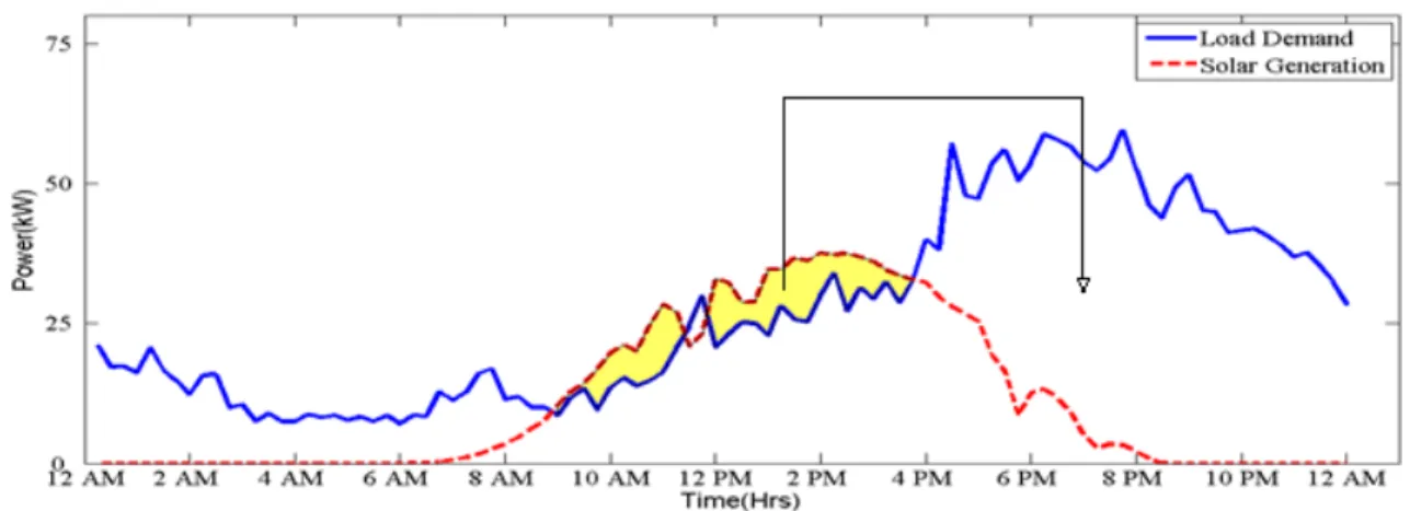
Figure 1.1. Load and solar profiles during the day. [1]

1. Synchronizing load and solar power profiles 2. Curbing the Duck curve

3. Economic factors

1.1.1. Synchronizing Load and Solar Power Profiles. Typically, the consumer

load has a common trend throughout the day. The load increases in the morning as everyone in the house wakes up and get ready for work. In the afternoon load demand decreases and again rises up to a second peak in the evening depending on the consumer’s lifestyle. On the contrary, the solar power output gradually increases in the morning, attains a maximum value at solar noon and reduces to zero in the evening (Figure 1.1). Without energy storage, surplus energy generated in the microgrid is fed back to the grid for which the utilities gives incentives to the customer. However, the costs of buying & selling electricity are different. The buying tariff is seven to ten times the selling tariff. From the economics point of view, the customer is buying the same electricity which was produced in the afternoon.

Due to the non-synchronized peaks of solar and load profiles, the renewable energy’s capabilities are not fully utilized. Therefore, energy systems can help overcoming such problems by storing the surplus energy and utilizing it when needed (Figure 1.2) using sophisticated control algorithms which will be discussed in the later chapters.

Figure 1.2. Store and utilize the surplus energy during peak load

1.1.2. Curbing the Duck Curve. In 2013, California ISO (Independent System

Operator) published a series of graphs projecting the future timing imbalance between peak load demand & renewable generation (Figure 1.3). The large scale installation of solar energy in the state of California has led to an imbalance of load demand during the solar peak and evening. The duck curve refers to the transition from solar peak to the sunset where the electricity generators needs to quickly ramp up the production during this time period. This leads to instability in the power system & higher operational cost. There are two solutions to this problem. One is at the macro level where different states/utilities can share load so that the load curve is consistent in power system. This solution is more complex & time consuming due to various economic and political hurdles. Another solution is at the micro level where the customer can locally install energy storage. The energy storage can store the surplus energy generated during solar peak hours and use it during load peak hours. This not only minimizes the imbalance between load demands during different times but also helps in peak shaving. This approach helps both the customers to lower down there monthly billing cost and also reduce operational cost for utilities which indirectly saves customer’s money.

Figure 1.3. Load demand projections for different years[2]

1.1.3. Economic Factors. We live in an economically driven society where every

product is bought with a motivation to have economic benefit from it. When a customer installs a microgrid, they expect some kind of service or a return of investment. Figure 1.4 depicts the ownership of microgrid by different sectors and the incentives they expect to receive. The top two motivations/expectations for installing a microgrid are system reliability and Cost reduction. As discussed in previous sections, solely using renewable energy cannot ensure cost reduction. Installing Energy storage not only ensures reliability but cost reduction too so that the consumer get return of investment in minimum possible time frame.

Figure 1.4. Microgrid ownership in different sectors and their motivation[3]

1.2. LITERATURE REVIEW

A Markov Decision Process (MDP) is a mathematical tool to take decision in systems where the outcome is partially stochastic & partially deterministic. MDP is widely popular in different areas of specialization from banking to biomedical engineering. The emergence of smart grids has called for implementation of MDP algorithms in microgrids too. Different problem statements might demand for different MDP models for the microgrids. For instance, in [6, 7], the authors discuss the problem of reducing the difference between the demand & the supply. At every time step, system takes a decision of meeting the power requirement either by renewable energy or the main grid. The MDP model is solved using Multi-Agent Q-Learning technique which doesn’t require any prior information of the system. [7] further discusses the difference between learning and Coordinated

Q-Learning where the objective function remains reducing the power consumption from the grid. Both of these research works do not include any forecasting models for load and solar. Rather, they depend on the immediate changes on the environment.

Research work presented in this thesis is more closely related to works in [8, 9]. In [9], the MDP optimally schedules the energy storage in power distribution including renewable resources. The output of the algorithm is an optimal policy for scheduling the energy system while minimizing the objective function, which includes total cost and the energy losses in the power system. Besides scheduling the battery using dynamic programming, this paper assesses & compares the battery system size optimal for a network operation.

Paper [10] formulates an optimal management & sizing of energy storage with dynamic pricing keeping dynamic pricing stochastic in nature. The algorithm solves the problem with minimum cost incurred to the customer keeping conversion losses, transmis-sion losses and investment costs into consideration. This paper also analyzes the size of the energy system vs its gains.

The MDP algorithm in microgrids runs for indefinite period of time. Therefore, a finite horizon problem i.e. an algorithm which optimizes only a finite time frame cannot work for microgrid applications. Therefore, infinite horizon or rolling horizon MDP is a feasible solutions for the given scenario. In [11], the Rolling horizon MDP algorithm in microgrids is presented with combined heating and power (CHP) generation to satisfy the electric & heat loads in the system.The research solves the problem with variable number of CHPs using greedy algorithm. The research work lacks the prediction of wind turbine output & load demand which is an integral part in implementing a practical energy management system.

Research work [12] presents an energy management system based on rolling horizon strategy with solar and wind as renewable resources. The energy system proposed also considers the SOH (State of Health) of the batteries which accounts for the investment and

the life of ESS. The paper also implements the load forecasting using Neural Network and solar forecasting using clear sky model integrated with MDP. The load and solar energy are stochastic in nature therefore the forecasting models cannot predict them accurately every time. Therefore simulating only one day of battery scheduling cannot accurately capture the performance of Energy Management System. Research work presented in this thesis attempts to develop the energy management system with MDP, Load forecasting using Auto-regressive Moving Average with Exogenous Input (ARIMAX) and solar forecasting using Non-Linear Auto-Regressive Exogenous Input (NARX) simulating for 30 days.

Load forecasting is a central area of interest for electric utilities and microgrids [13, 14, 15]. Time series models, which include a linear combination of past values and Gaussian errors, have been widely popular in the research community for short-term load forecasting. [16] implements a short-term load forecasting using ARIMA model & transfer function model by considering the weather forecast. It formulates models for different sectors like residential, commercial and industrial loads. The transfer function relationship between load and weather are different for different sectors therefore, different models are required. The paper concludes that the transfer function ARIMA models perform better than the ARIMA models.

Paper [17], analyzes nine different methods for short-term load forecasting like regression, adaptive load forecasting, stochastic time-series, fuzzy logic, etc. The research concludes that the load forecasting models require more sophisticated forecasting models with an inclination towards stochastic & dynamic forecasting techniques. There is also a trend towards developing hybrid models which combine two or more techniques to extract the best features of these techniques.

Similar forecasting techniques are applied to Solar forecasting too. Either the solar radiation is predicted or the PV output is predicted directly using various forecasting models. Time series models have been well used in solar forecasting [18, 19, 20]. The solar energy is partially predictive due the Earth-Sun geometry constraints and partially stochastic due

its dependence on surrounding environment like clouds & nearby materials. Therefore, traditional models tend to fail. Techniques like Neural Networks and Support Vector Machines are used for solar forecasting due to their abilities to capture the non-linearity and non-stationarity of the time series.

Paper[21], presents a comparison between multi linear analysis model, Persistence and Neural network model. Multi linear model is a regression of various parameters affecting the solar radiation like temperature, humidity, time of day, etc. Persistence model as the name suggests is obtained by keeping the actual value constant for the current hour and using it for the forecast. Though this technique works for very short-term forecasting but if the prediction window is large, this technique fails. The Artificial Neural Network models have better accuracy than the multi liner and Persistence models.

Paper [22] presents a Neural network model for PV output forecasting taking ex-ogenous time series like temperature, humidity, Pressure, cloud cover and past observed PV output into consideration. These are also called Non-Linear Autoregressive Neural Network (NARX) models. The paper further studies the Mean Average Error (MAE) in different cloud conditions. The research presented in this thesis has adopted this technique for implementation of Energy Management System.

1.3. ORGANIZATION OF THE THESIS

In addition to the section 1, which represents the motivation of using battery sys-tems in microgrids, need of energy syssys-tems and literature review, section 2 presents the formulation of the microgrid system and there mathematical constraints. Markov Decision Process is discussed in reference to the microgrids and mathematical framework behind the implementation of the same. The implementation of MDP in microgrid is discussed with zero forecasting errors to obtain a proof of concept and the theoretical limitations of the system.

Section 3 discusses load forecasting techniques like ARIMA (Auto Regressive Mov-ing Average), SARIMA ( Seasonal Auto Regressive MovMov-ing Average) & ARIMAX (Auto Regressive Moving Average with Exogenous time series) models. The implementation of the load forecasting models is presented and results of a one month load forecasting simulation is shown. Chapter 4 presents the solar forecasting techniques. Clear Sky model, Multi linear model and Auto Regressive Exogenous Neural Network Models are discussed and compared.

Section 4 shows the implementation of the Energy Management system by integrat-ing MDP, Load & Solar forecastintegrat-ing. The Energy Management system presented in this thesis is compared with a Heuristic approach which does not require any intelligent control.

2.1. SYSTEM MODELING

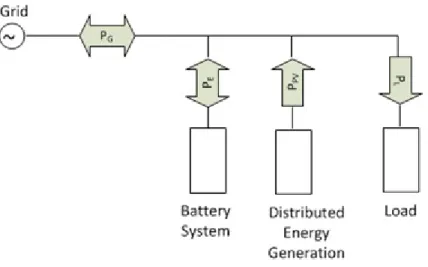
The system under consideration contains a local load, PV source, battery system and grid connection. System is shown in Figure 2.1. Arrows describe the flow of energy. Solar (PPV)and load power (PL) flows are unidirectional and only take positive values. Whereas

the power flows of Grid (PG) and battery system (PE) are bidirectional and can take both

positive and negative values. Grid power (PG) is positive when energy is drawn from it

and negative when surplus energy is fed into the grid. Similarly, Battery power (PE) is

positive when it is discharged and negative when charged. Solar output power (PPV) and

Load demand (PL) are always positive. The system operates with the following constraints: PL −PG−PE −PPV =0 (2.1) SoCmin ≤ SoC(k) ≤SoCmax (2.2) P_Emin ≤ PE ≤ PEmax (2.3)

The Battery power (PE) is bounded by maximum and minimum powers P_Emax & P_Eminrespectively. The State of Charge (SoC(k)) at any time stepkcannot exceed minimum

(SoCmin) and maximum (SoCmax) values based on battery specifications.

2.2. MARKOV DECISION PROCESS

Markov Decision Processes (MDPs) are a class of stochastic sequential decision processes in which the cost and transition functions depend only on the current state of the system and the current action [8]. As load demand and PV generation are uncertain in

Figure 2.1. System architecture

nature, MDP is a good option to schedule the battery charging/discharging rate. A day is discretized into 15 minutes interval i.e. 96 epochs thereby reducing the problem statement to making 96 decisions of charging/discharging battery rate in 24 hours. Rolling Horizon MDP is implemented in the system to ensure that the control algorithm always keeps 24 hours into consideration while making a battery action.

The state,sk, at epochkhas all the information necessary to define cost and transition

probabilities

sk = {E,uˆPV,σˆPV,uˆL,σˆL, θs, θb,k} (2.4)

where,

E = Discretized energy of battery in kWh

ˆ

uPV = Point forecast of PV Generation in kW

ˆ

σPV = Standard error of PV Generation in kW

ˆ

uL = Point forecast of Load demand in kW

ˆ

θs= Electricity selling cost in $/kW θb= Electricity buying cost in $/kW k is the epoch

2.2.1. Battery Energy. During transitions between epochs,_buPV ,bσPV, ˆuL, ˆσL, θs,

andθbare independent of control actions and are deterministic. Therefore, state transitions

are determined by the change in battery energy, e(t). To facilitate calculation, energy is

discretized into M bins of size.

Ebin=

E_max−E_min

M (2.5)

So, a battery can have energy (state)Ei as:

Li = Emin+(i−1)Ebin (2.6) Ui = Emin+iEbin (2.7) Li ≤ e(t) ≤Ui (2.8) Ui is the upper limit of Energy at E = i and Li is the lower limit of Battery Energy at E = i. Therefore battery can have M discrete states during the scheduling and energye(t)

of battery would be greater thanLi and smaller thanUi. In the simulations, M is taken as

200, Emax as 200 kWh and Emin as zero but during practical implementation, boundaries

can be set onEmax &Eminto ensure that the battery is charged/discharged till certain levels. 2.2.2. Battery Actions. In MDP formulation for battery scheduling, actions(n) is

considered to be Charging/Discharging rate in kWh. This is defined by the specification of the battery system. From each stateEi, some finite discrete actions are possible. These

in energy E with a probability of 1 (Equation 2.9). Pi j =        1 i f (i− j)= n 0 i f (i− j)_, n (2.9)

Where,iis the state at epoch k and j is the state at epochk +1. The action in kWh can be

computed by referring to the specification of the Battery system (Equation 2.10).

PE =        nEbinηd ∆t nE_bin ∆tηc n> 0 n< 0 (2.10) where,

PE is battery charging/discharging power

ηd&ηcare discharging and charging efficiency respectively

∆t is the time interval between two actions (15 minutes in our case)

2.2.3. Cost. Total cost accumulated at each state denoted byCi j,kof a certain epoch

is a function of destination state of the next epoch and the action taken. It is to be noted that the cost mentioned here is not the actual cost of the day. Rather, it is divided into two parts:

1. Grid Cost

2. Energy Transfer Cost

2.2.3.1. Grid cost. This is the expected cost by transitioning from stateEitoEj at

epochk.

Now,PG is estimated by the following constraint:

PG = PL −PPV −PE (2.11) PE is held constant. Distribution of PG is Gaussian with following parameters:

ˆ

ˆ σG = q ˆ σ2 L+σˆPV2 (2.13)

There are majorly two types of rate structures imposed by utilities on customers: 1) Time of Use (TOU) rate: In this structure, the prices are increased during peak load periods. For example, utilities might have peak period from 12:00 PM to 7:00 PM when the demand is the highest. Purchase price for the off peak hours would be lower than the on-peak hours thereby encouraging customers to consume less power during those periods. Cost associated with this scheme for a particular epoch withPE held constant is as follows:

CG =        PGθs∆t PG <0 PGθb∆t PG > 0 (2.14) Where,∆t is the size of one epoch which is 15 minutes in this study. The expected cost of CG is given in Equation 2.15 E[CG]= 0 ∫ −∞ θs∆t x √ 2πσˆG exp −(x− µˆG)2 2 ˆσ2 G ! dx+ ∞ ∫ 0 θb∆t x √ 2πσˆG exp −(x− µˆG)2 2 ˆσ2 G ! dx (2.15) E[CG]= ˆ µG∆t √ 2 ˆσG " (θ_b−θ_s) σˆG ˆ µG r 2 π exp −µˆ2_G 2 ˆσ2 G ! +erf µˆG √ 2 ˆσG ! ! +θb+θs # (2.16) 2) Demand charge: This charge is generally levied on Industrial/commercial facil-ities or customers with high power consumption. Some utilfacil-ities in states like Alabama, Arizona, Wyoming, California and many more [23] have implemented demand rate struc-ture for residential customers too. Bill is generated on the basis of two components, first is fixed rate where the purchase rate remains constants throughout the billing cycle. Second

is the demand rate which accounts for a large amount in the bill. Demand charge is based on the highest power consumed in a 15 min duration for one month billing cycle. The Cost associated with this rate structure is as follows:

CG=                PGθs∆t PG <0 PGθb∆t 0 < PG < γ (PG −γ)θd∆t+γθb∆t PG > γ (2.17) where, θs= Selling price in $/kWh θb= Buying price in $/kWh θd= Demand charge in $/kWh

γ= Threshold value for demand in kWh

Expected cost ofCG is given in Equation 2.18 and 2.19. In this research, Demand

charge rate structure is going to be followed.

E[CG]= θs∆t √ 2πσˆG 0 ∫ −∞ xexp −(x−µˆG) 2 2 ˆσ2 G ! dx+√θb∆t 2πσˆG γ ∫ 0 xexp −(x−µˆG) 2 2 ˆσ2 G ! dx + θd∆t √ 2πσˆG ∞ ∫ γ xexp −(x−µˆG) 2 2 ˆσ2 G ! dx (2.18) E[CG]= (θ_d−θ_s) 2 σˆG r 2 π exp −(γ− µˆ_G)2 2 ˆσ2 G ! +(γ−µˆ_G)erf γ√− µˆG 2 ˆσG ! +γ ! +(θb−θs) 2 σˆG r 2 π exp −(µˆG)2 2 ˆσ2 G ! +µˆGerf ˆ µG √ 2 ˆσG ! ! + µˆG(θd+θs) 2 (2.19)

2.2.3.2. Energy transfer cost. This is the cost of Energy transfer from/to battery

to emphasize on the notion that the battery is degraded while charging/discharging it and enabling the MDP to determine whether it is financially advantageous to supply the load with grid energy or battery energy. Battery costCBis defined as :

CB = Ebin(i− j)θe (2.20)

where,

θe= Energy transfer cost in $/kWh i= Initial energy state at epoch k

j= Final energy state at epoch (k+1)

From Equation 2.20, the cost is positive when j < iand negative when j > i. The

primary objective of the system is to attain least cost. Therefore, this cost term tries to attain higher SoC (State of Charge) of the battery which heavily dependent onθe.[24, 25],

estimate the value ofθe by considering the battery installation cost and lifetime. Though

it is out of the scope of this study but SoC and SoH (State of Health) estimation can be implemented in this topology to calculateθefor considering the degradation and lifetime of

battery system. The total cost for transitioning from state “i” to “j” at epoch “k” is described in Equation 2.21.

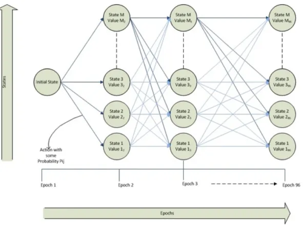
Ci j,k =CG +CB (2.21) 2.2.4. Optimal Policy. Dynamic programming is used to calculate the optimal

policy of the MDP. The tree diagram shown in Figure 2.2 summarizes the implementation of MDP in microgrid. The optimal policy of each state at epoch k is defined by the Bellman equation. U_i∗_,k =min nA M Õ j=1 Pi j(Ci j,n+U∗_j,k+1) (2.22)

Figure 2.2. Implementation of MDP using Dynamic Programming U_i∗_,K =−θ_e(E_min+(i−0.5)Ebin) (2.23) a_i∗_,k =argmin n∈A M Õ j=1 Pi j(Ci j,n+U∗_j,k+1) (2.24)

Where,Ui,Kis the optimal utility at epochkand state i, K is the last epoch (e.g. 96), anda∗_i,k

is the optimal action at epochkand statei. Actions determined by Equation 2.24 determine

the optimal policy for the battery controller. Since the terminal cost is based on the energy, the system prioritizes high battery energy at the end of the horizon while reducing the grid cost.

Rolling Horizon MDP ensures that there is always enough energy in the battery system to supply day ahead load demand taking into consideration both solar output and load demand.

2.3. IMPLEMENTATION

To validate the performance of MDP model and obtain a theoretical limit of the system, forecasting errors are ignored. In other words, MDP model is integrated with load and solar forecasting models which have zero forecasting errors. The load & solar data are taken from a research facility Pecan Street dataport situated in Austin. A community of 20 houses is considered with 10 houses having PV panels installed. demand charge rate structure is imposed using parameters from RMU (Rolla Municipal Utilities) given in Table 2.1. The battery system is assumed to have a capacity of 200 kWh with an initial SoC of 50%. The battery system has maximum charging power of 68.4 kW and maximum charging capacity of 75.7 kW.

Table 2.1. Demand rate structure used in simulations (Adopted from Rolla Municipal Utilities)

Parameter Rate

Buying Rate (θb) ($/kWh) 0.07009

Selling Rate (θs) ($/kWh) 0.01326

Demand Rate (θd) ($/kW) 14.5

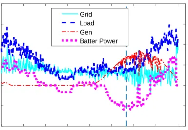
It can be observed from Figure 2.3 & 2.4 that the solar output is stored in battery bank during surplus generation and the same energy is used during peak load. This helps to maintain constant power drawn from the grid and reduce the maximum peak power. This in turn reduces the demand charge in the system. Table 2.2 shows the cost comparison of system with & without MDP & battery system.

7 PM 10 PM 1 AM 4 AM 7 AM 10 AM 1 PM 4 PM 7 PM Time(Hrs) -50 -25 0 25 50 75 100 Power(kW) Grid Load Gen Batter Power

Figure 2.3. MDP simulation for one day

Figure 2.4. Comparison between the grid powers of system with & without MDP. Old grid is the system without MDP & battery system

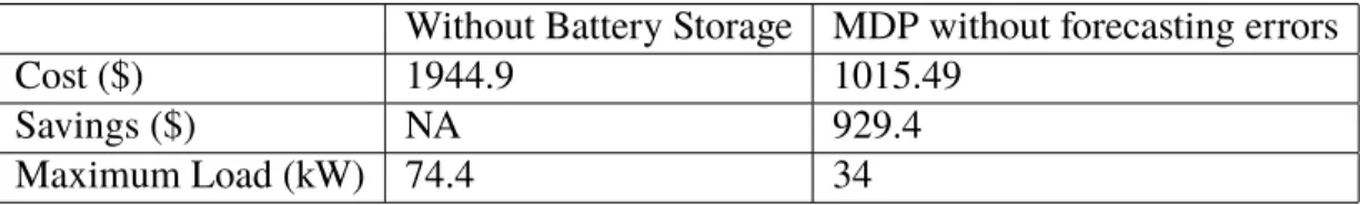
Table 2.2. MDP one month simulation results

Without Battery Storage MDP without forecasting errors

Cost ($) 1944.9 1015.49

Savings ($) NA 929.4

Maximum Load (kW) 74.4 34

It can be observed from Table 2.2 that the system with no battery pack has a maximum load demand of 74.4 kW. Whereas, a system with battery pack and MDP algorithm reduces the maximum load demand to 34.6 kW thereby saving $929.4 in one month. Though, this model only signifies the capabilities of MDP algorithm & a theoretical limit to the cost savings. The MDP model is incomplete without load and solar forecasting models. Therefore, forecasting models are discussed in proceeding chapters in order to integrate them with MDP.

Load forecasting is a tool used by utilities and power companies for planning & op-eration of power systems. Increased acceptability of microgrids has encouraged researchers to forecast loads at a micro level for energy control purposes and increase the penetration of renewable energies in the microgrid system. Load forecasting captures the customer behavior and predicts load with a lead time from several minutes to even days depending on the application. Load forecasting can be categorized based on the forecast horizon:

1. Short term forecast: The prediction period ranges from several minutes to weeks. It is generally used for Network planning, supply/demand matching, load shedding strategy, etc.

2. Medium term forecast: The prediction period ranges from weeks to months. The main advantages of medium term forecast are network planning, power procurement & rate case development.

3. Long term forecast: The prediction window ranges from months to years. Long term forecasting is generally used by power companies for investment planning and projecting the need for infrastructure.

The system load in a microgrid is the sum of all individual loads of all houses forming a microgrid. In principle, if the characteristic consumption of individual house is known, load can be predicted easily. The total load in a microgrid results in distinct features which can be statistically predicted.The load pattern is influenced by a number of factors which are listed below:

1. Economic: Economic factors have different meaning for different sectors where load forecasting is performed. For microgrids, the rate structure imposed by the utilites is crucial. For example, in case of Time of Use (TOU) rate structure, consumer

will try to maintain low load demand during specific times. Whereas, in case of Demand charge structure customer will try to maintain low load demand peak (flatter consumption profile). Therefore, knowing the economic factors can play a key role in predicting the future load demand .

2. Time: The consumer load has a specific profile which can be extracted from the time of prediction. The load profile therefore repeats itself after every 24 hours. This is called seasonality. Even if the consumer’s load consumption pattern changes, it is updated on the next day’s forecasting results. Other time factors affecting the load profile are weekends, holidays like Christmas and special events like the Super Bowl. 3. Weather: Meteorological changes are major factors affecting load consumption due to the presence of weather sensitive components in the system, particularly air con-ditioning and space heating. The inputs for the load forecasting can be temperature, humidity, dew point & wind speed. However, not all weather parameters can have correlation with the load consumption. Analysis is needed to decide which weather parameters directly affect the load consumption.

4. Stochasticity: Random behavior of the customer or event can cause a change in load consumption which cannot be explained from the other factors discussed above. This property largely calls for the load forecasting models.

3.1. LOAD FORECASTING MODELS

Load forecasting can be performed with different models like multiple regression technique [13, 26], Time series model & Artificial Neural Networks. Time series models are the classical approach to load forecasting. It is a linear combination of past observed values of the load demand. Time series models are relatively simple compared to the Artificial

intelligence (AI) methods and produces same accuracy as that of the AI models [27]. This research work focuses on developing a Time series model for load forecasting due to its simple mathematical framework and wide acceptability for practical applications.

3.1.1. Time Series Models. Time series is defined as the series of data generated

sequentially in time [28]. The time series models assume that the future data is related to the past observed values of the time series.

Introduced by Box and Jenkins [29], ARIMA (Auto Regressive Integrated Moving Average) modeling has been a popular technique to predict the future load demand [30]. ARIMA model has three components: Autoregressive (AR), Moving Average (MA) and differencing.

The primary requirement of the ARIMA model is that the time series has to be stationary. In other words, a time series is stationary if the statistical properties (mean, variance, autocorrelation) do not change with time. Kwiatkowski−Phillipsi−Schmidti−Shin

(KPSS), Dickey−Fuller test (ADF) and unit root test are the common methods to determine

the stationarity of a time series. Mathematical operations are needed to be performed if the time series is not stationary. A non-stationary time series can be made stationary by differencing the data set with various methods like normal differencing, exponential smoothing, regressing on trends, etc. In most of the cases, one or two differencing is enough to make a series stationary. The order of differencing is denoted by “d”.

Ifd = 1, the time series is stationary.

yk =Yk (3.1)

Ifd = 1, the series is differenced with itself once.

Ifd = 2, the time series is differenced twice.

yk =(Yk −Yk−1) − (Yk−1−Yk−2)=Yk−2Yk−1+Yk−2 (3.3) where,

yk is the stationary series obtained after differencing Yk is the original time series

k is the discretized time step

It can be observed that as the differencing order increases, the equations also become complex. Therefore, to make the time series equations easy to perceive, a lag operator “B” is introduced (Equation 3.4). Operator “B” is similar to thez−1operator in discrete domain. BYk =Yk−1 BmYk =Yk−m (3.4)

Therefore, a one and two differencing equations (Equation 3.5 & 3.6) can be represented as follows:

yk =(1−B)Yk =Yk −BYk (3.5) yk = (1−B)2Yk =Yk −2BYk +B2Yk (3.6)

Autoregressive (AR) component stresses on the fact that the present value of the load demand is related to the past observed values. It is weighted sum of past observed/forecast values of the time series. The order of autoregressive model (p) is determined using partial

autocorrelation. The Moving average (MA) term is a weighted sum of the forecast errors. The order of MA (q) is determined from auto-correlation plots.

Though, the partial correlation and auto correlation plots gives a ballpark numbers for the orders of AR & MA orders respectively.Figure 3.1 & Figure 3.2 shows the pacf & acf plots of a stationary time series.

0 10 20 30 40 50 Lag -0.4 -0.2 0 0.2 0.4 0.6 0.8 1 Sample Autocorrelation

Sample Autocorrelation Function

Figure 3.1. Auto correlation of stationary time series

It can be observed from Figure 3.1 & 3.2, that the auto correlation and partial correlation damps to zero after some lags. These lags can be used as ball park numbers to start with the AR & MA lags. Though these might not be the actual orders but it helps to look for the starting point. During the modeling phase, different combinations of MA & AR orders are tested and the model with highest accuracy is chosen. ARIMA equation is represented as follows: φ(p)(1−B)d(Yk −u)= ϕ(q) (3.7) φ(p)= 1− i=p Õ i=1 φiBi ϕ(q)=1+ i=q Õ i=1 ϕiBi (3.8) where,

Yk is time series to be predicted φ(p)is the Autoregressive function

φiis the autoregressive coefficient ϕiis the moving average coefficient ϕ(q)is the Moving Average function

uis constant or intercept dis differencing order pis autoregressive order qis moving average order

3.1.2. Seasonality. Load trends are seasonal in nature. Present data is correlated

with previous day’s data. Addition of seasonal terms in time series forecasting increases the accuracy of forecasting model. There is no formal method of calculating the order of seasonality. It can be observed by carefully studying the time series trend and looking for highest past cross correlation function (Figure 3.3). Plotting frequency spectrum of the time series can also help in investigating the seasonality of data set. In Figure 3.3, a load

-200 -100 0 100 200 Lag -1 -0.5 0 0.5 1

Sample Cross Correlation

Sample Cross Correlation Function

X: -96 Y: 0.7909

Figure 3.3. Cross-correlation of original time series

data set is discretized into 15 minutes intervals/epochs and shows that the current value is highly correlated with the past 96th epoch/past 24 hour value. This also makes sense as the typical load behavior of a consumer load does not change on a daily basis.

Therefore, the past 24 hours load value can also be used to predict the future load. Seasonality integrated with ARIMA model is called SARIMA (Seasonal Auto Regressive Integrated Moving Average) Model. The equation of SARIMA model is given below

φ(p)φ_s(P)(1−BS)D(1−B)d(Yk−u)= ϕ(q)ϕs(Q) (3.9) φs(P)=1− i=P Õ i=1 φs iB i _ϕ( Q)=1+ i=Q Õ i=1 ϕs iB i _(3.10) where,

φ(P)is the Seasonal Autoregressive function

φs

i is the autoregressive coefficient ϕs

i is the moving average coefficient ϕ(Q)is the Moving Average function

Sis the seasonality of time series

Dis the seasonal differencing of time series Pis the order of Seasonal Autoregressive function Qis the order of Seasonal Moving Average function

The coefficients of SARIMA model is calculated using SAS (Statistical Analysis Tool). Other software tools like MATLAB & R can also be used for this purpose. Equation 3.9 is represented asARI M A(p,d,q)S(P,D,Q)in short. Different SARIMA were tried and

model withARI M A(5,1,5)96(0,1,1)produced the best accuracy. Simulations for 24 hours

ahead load forecasting is performed for one month data where the model is updated every 15minutes. Mean Average Percentage Error (MAPE) (Equation 3.15) histogram is plotted for the simulations. The histogram (Figure 3.4) represents the MAPE of 2500 day-ahead load forecasting. The minimum MAPE of the simulation is 9.7131% and the maximum MAPE is 81.9178%. As the SARIMA model predicts the future load by regressing the past value, it fails to predict the future load change due to external factors like weather. Therefore, weather parameters are important to be integrated in the system to accurately forecast the load demand.

3.1.3. Weather Correlation. Among all the dependent factor of load

consump-tions, weather dependent load plays a vital role in short-term load forecasting [19]. Weather components can constitute Temeprature, Humidity, Wind speed, dew point, etc. Though it depends on the consumer load and behavior which needs to be investigated before including the weather factors.

The data set being used in this research work only has correlation with temperature (0.8466) with a lag of 150 minutes. This means that the load demands react to the temperature changes after 150 minutes. Figure 3.5 shows that the load is linearly dependent on temperature but it is not necessary for all load demands. Some load demand might have a quadratic or even no relationship with load. Therefore, a thorough analysis is necessary while choosing the weather parameters.

0 20 40 60 80 100 MAPE (%) 0 5 10 15 20 25 30 35 40 Frequency (%)

Figure 3.4. SARIMA model one month

0 10 20 30 40 50 60 70 80 Temperature (Fahrenheit) 60 65 70 75 80 85 90 95 Load (kW)

3.2. LOAD FORECASTING MODELING

Load forecasting involves two steps i.e. formulating a relationship between load -weather parameters (Regression Method) and predicting the residuals regression method using SARIMA model. For example, the regression model obtained from the data set is a linear equation between load and temperature (Equation 3.11).

b

X[k]=u+aT emp×T[k−10] (3.11)

where,

X[k]is the load predicted using regression method

uis the intercept equal to -129.698 for the data set taken into consideration aT empis the regression factor of Temperature equal to 1.945

T[k]is the temperature expressed in Fahrenheit

The temperature forecast is obtained from the weather stations which predict the weather for next 48 hours. Various weather stations provide with APIs which can be used to acquire the weather forecast (Appendix-A).

The residual error after applying (Equation 3.11) is predicted using SARIMA of the form SARIMA(5,1,5)X(0,1,0)96 (Equation 3.12). This form gave the best accuracy for the given data. φ(p)(1−B96)(1−B)( b ek −u)= ϕ(q) (3.12) φ(p)= 1− i=5 Õ i=1 φiBi ϕ(q)=1+ i=5 Õ i=1 ϕiBi (3.13)

The error/residuals predicted (Equation 3.12) using SARIMA model are added to the load predicted using regression model (Equation 3.11). The addition of both the models results into the final prediction of the load (Equaiton 3.14).

Figure 3.6. Load forecasting approach

The parameters in Equation 3.11 & 3.12 are obtained from SAS software. The flow diagram of the load prediction is depicted in Figure 3.6.

ˆ

Y[k]= Xˆ[k]+eˆ[k] (3.14)

where,

Y[k]is the load forecasted at epoch/time step k X[k]is the load predicted using regression model

0 20 40 60 80 100 MAPE (%) 0 5 10 15 20 25 30 35 Percentage (%)

Figure 3.7. One month simulation MAPE result of load forecasting

3.3. RESULTS

The load data was obtained from Pecan Street data port. The minutely data is converted to 15 minutes averaged data. The aim of the forecasting model is to predict 24 hours ahead load demand from the current epoch. This reduces to predicting future 96 epochs of load demand. SARIMA model discussed in previous sections is used for load predictions . The forecasting model is analyzed based on MAPE (Mean Average Percentage Error) (Equation. 3.15) M APE = 1 96 k=96 Õ k=1 Y[k] −Yˆ[k] Y[k] ×100 (3.15)

For day-ahead load forecasting updated every 15 min for 30 days, simulation results show MAPE (mean absolute percentage error) within 30% for 95% of the epochs (Figure 3.7), with a highest MAPE of 36.2% and lowest MAPE of 10%. It can be observed that the

temperature parameters act as the backbone of load forecasting thereby effectively predicting the future load trend. SARIMA model is applied on top of the load predicted using weather parameter to improve the forecasting.

Solar energy is one of the most abundant renewable energy in the United States. Since 2008, US solar installation have grown from 1.2 GW to 30 GW which is enough to power 5.7 million American home. The PV panels have also become affordable as their price dropped by more than 60% in the past decade (Figure 4.1). Based on average prices, the system cost of installing solar panels in the US is $3.14/watt.

GTM (Green Tech Media) research suggests that the solar installation cost in India has reached as low as 65 cents per watt. Increased popularity, tax incentives, cutting edge technology are some of the reasons contributing to cheaper solar panels.

Solar energy integrated with microgrids improves the reliability of the system too. For example, in case of storms, the infrastructure of power systems is destructed due to which the solar panels directly tied to the power system stop working too. Microgrids have are more advanced and prepared for such scenarios and there smart software senses the incoming disruption. They isolate the microgrid from the power system and directly rely on their solar power and battery systems till the power system is again operating. Therefore, microgrids integrated with solar power not only provide green energy, cost reduction but also increases the reliability of the system.

All these factors contribute in encouraging the microgrid customers to install solar panels in their systems. Though, having solar panel in the system is not enough. In order to increase the penetration of solar energy, one needs to predict the upcoming solar power to better manage the energy output. There are a few solar terminologies which are needed to be discussed before discussing the forecasting models.

Figure 4.1. Solar panel cost reduction trend[4]

4.1. FUNDAMENTAL CONSIDERATIONS

Before diving into the solar forecasting methodologies, basic terminologies are dis-cussed in this section.

1. Declination Angle (δ): Solar declination is the angular distance between the equatorial plane and the earth-sun line (Figure 4.2). Declination angle varies from+23.45◦ _to

−23.45◦throughout the year. Solar declination can be defined as a function of day in

a year as follows: δ= 23.45×sin 360◦(n+284) 365 (4.1) where,

n=Day of the year (n=1 for 1st Jan, n=32 for 1st Feb, etc) δand angle inside sin are in degrees

Figure 4.2. Declination angle of earth is different at different times of the day

2. Hour Angle (ω): Hour angle is an expression of observing the Sun from Earth through-out the day. It is expressed in degrees. At solar noon, hour angle is equal to 0 degrees. Time before solar noon is expressed in negative and after solar noon is expressed in positive. Sunrise/Sunset hour angle equation is described in Equation(4.2).

cos(ω_o)= −tan(ϕ)tan(δ) (4.2)

where,

ωois Sunset/Sunrise hour angle (Negative for sunrise and positive for sunset) ϕis Latitude of the location of interest

Earth rotates at an angular velocity of 15◦ _{hour angle/hour. Therefore, if the time} of the day is known, hour angle can be calculated accordingly. Hour angle has the following constrain at a particular day:

3. Solar Altitude (β): Solar Altitude is the angle between the horizontal plane and the line which joins the point of interest with the Sun (Figure 4.3). Expression for solar angle is given in Equation(4.4).

sin(β)=cos(ϕ)cos(δ)cos(ω)+sin(ϕ)sin(δ) (4.4)

where,βis Solar altitude

4. Zenith angle (φ): It is the angle between the vertical plane and line which joins the point of interest with the Sun (Figure 4.3). Therefore, Zenith angle and Sun altitude angle are co-dependent (Equation 4.5).

φ= 90− β (4.5)

5. Azimuth Angle (θ): Azimuth angle is defined as the angular displacement of the projection of earth-sun line with south on the horizontal plane (Figure 4.3). Azimuth angle can be computed from Equation 4.6.

cos(θ)= (cos(ω)cos(δ)sin(ϕ) −sin(δ)sin(ϕ))

cos(φ) (4.6)

where,θis the Azimuthal angle

6. Extraterrestrial Solar Radiation: Extraterrestrial Solar Radiation Eo is the solar

ra-diation flux just outside the EarthâĂŹ‘s atmosphere. Due to the elliptical path of Earth‘s orbit,Eois not constant throughout the year, but can be approximated by

Eo= Esc 1+0.033∗cos 360◦n−3 365 (4.7)

Figure 4.3. Solar Angles for horizontal and vertical surfaces[5]

where,

Esc = Solar constant (1367W/m2)

n = Day of the year (n=1 for 1st Jan, n=32 for 1st Feb, etc)

7. Air mass (m): It is the ratio of the actual air mass present in the atmosphere to the

air mass that would be present when the sun was directly overhead. Air mass is the function of solar altitude (Equation 4.8)

m= 1

sin(β)+0.50572(6.07995+β)−1.6364 (4.8)

4.2. FORECASTING MODELS

Total extraterrestrial solar radiation is the solar radiation received by the outer atmosphere of the Earth which fluctuates around the average value of 1360W/m2. This

radiation is attenuated in the atmosphere by complex reflections, refractions and absorptions by various factors like clouds, aerosols, air mass, etc. Therefore, there involves a challenge in predicting the solar radiation received by the surface of the due to its complex attenuation by the atmosphere. This research work discusses three major methods to predict day ahead solar radiation / solar power output in the system i.e. Clear Sky Model, Regression Model and Non-Linear Autoregressive Neural Network Model.

4.2.1. Clear Sky Model. ASHRAE (The American Society of Heating,

Refrig-erating and Air-Conditioning Engineers) [16] clear sky model estimates the Global solar radiation assuming that there are no clouds present in the sky[31, 32, 33]. Broadly, Global solar radiation on a clear sky day is defined as the sum of direct solar beam and the diffused beam from the sun. These two radiances are described as follows:

Eb= E0exp[−τbmab] (4.9) Ed = E0exp[−τdmad] (4.10) ab=1.454−0.406τb−0.268τd+0.021τbτd (4.11) ad =0.507+0.205τb−0.080τd−0.190τbτd (4.12)

Where,

Ebis the direct radiation. It is the radiation directly coming from the Sun in a straight line

to the surface of the Earth (Measured perpendicular to Sun rays).

Edis the Diffused solar radiation which is scattered by the atmospheric particles (Measured

horizontal to the surface)

m= Air Mass

τb&τd are the Pseudo optical depths. These values also considers the atmospheric effects

of the location. ASHRAE handbook-fundamentals provides these values for each month based on the site. These values are updated every year for better accuracy.

ab&ad are the beam and diffused air mass exponents.

4.2.1.1. Calculation of incident radiation on a surface. Total Global radiation

on a surface inclined to the horizontal plane is defined as the sum of the Direct radiation, Diffused radiation and Reflected radiation.

Et = Et,b+Et,d+Et,r (4.13)

where,

Et = Global solar radiation

Et,b= Radiation directly originating from the sun Et,d = Radiation diffused by the EarthâĂŹs atmosphere Et,r = Radiation after getting reflected from the ground

Et,b= Ebcos(θi) (4.14) Ebis direct beam radiation described in Equation 4.9 andθiis the angle of incidence which

can be calculated from the relationship given in Equation 4.15

cos(θ_i)=cos(β)cos(θ)sin(α)+sin(β)cos(α) (4.15)

where,

θis Effective Azimuth Angle

αis Angle of tilt of the surface from ground

Et,d = Ed(Y sin(α)+cos(α)) (4.16) Y = max 0.45,0.55+0.437cos(θ)+0.313cos2(θ) (4.17) It is to be noted that Equation 4.14 and 4.16 are a modified versions of Equation 4.9 & 4.10 respectively to calculate the Solar radiations in case surface/PV panel is placed in a certain orientation w.r.t. to the horizontal plane

Et,r =

(Ebsin(β)+Ed)ρg(1−cos(β))

2 (4.18)

Where, ρg is the coefficient of ground reflectance. It has been empirically calculated for

different surfaces which can be found in ASHRAE handbook-fundamentals.

4.2.1.2. Clear sky model results. Solar power output is directly proportional to

the solar radiation incident on the PV panel (Equation 4.19)

Out put Power = Solar_Radiation×Ar ea×E f f iciency (4.19)

Preliminary requirement in case of clear sky model is to predict the solar radiation accurately. Core assumption of clear sky model is that there should be no clouds in the sky. Therefore ASHRAE model gives best performance on days without no clouds but fails to predict the solar radiation on cloudy days.

Therefore, it is necessary to add some external factors in the solar forecasts. ASHRAE model alone cannot be used to predict the solar output but it can act as a backbone structure to predict the solar radiation which will be discussed in following sections.

4.2.2. Regression Model. Solar radiation is dependent on Earth-Sun geometry, the

cloud cover and the weather[34, 35, 36]. Therefore, if the weather is known beforehand, solar radiation can also be predicted. Weather stations have past years weather data base, satellite imageries and complex algorithms to predict the weather with up to one week

Figure 4.4. Solar radiation & Relative humidity are linearly correlated with a correlation coefficient of -0.8402

of prediction window. Most of the weather stations provide APIs to give 48 hours ahead weather forecast with a time step of one hour. Though, the weather is affected by the solar radiation but if we can use the reverse technique and predict the solar radiation from the predicted weather. Weather stations mostly provide with temperature, relative humidity, dew point, wind speed, precipitation, etc. The correlation between solar radiation/solar power output and other weather parameters are needed to be analyzed before moving to the modeling part. From the available dataset, temperature (Figure 4.4) and humidity (Figure 4.5) had the highest correlation with solar radiation.

Clear sky model gives the solar radiation available on a clear sky day. This means that it is the maximum solar radiation that is incident on the surface of solar panel. Therefore, ASHRAE clear sky model is taken as a reference and regressed against temperature and relative humidity forecasts. ASHRAE model consists all the necessary information for predicting the solar radiation such as latitude, time of day, air mass, reflectivity around the PV panel, etc. Rest of the information like weather parameters, efficiency of PV panel, area

Figure 4.5. Solar radiation & Temperature are linearly correlated with a correlation coefficient of 0.7429

of PV panel is included in the model using Regression model (Equation 4.20)

Sk = µ+ ASH RAEk ×α+T emper atur ek× β+Humidityk × χ (4.20)

where,

Sk is the predicted solar radiation at epochk

ASH RAEk is the ASHRAE model prediction at epochk

T emper atur ek is the temperature forecast at epoch kacquired from weather station Humidityk is the relative humidity forecast at epochk acquired from weather station µis the intercept equal to 345.36433 for available dataset

αis the regression factor of ASHRAE model 0.59383 for available dataset

βis the regression coefficient of temperature forecast 2.44879 for available dataset

Figure 4.6. Regression model flow diagram

Regression factors are calculated using SAS software. The performance of solar output is analyzed based on NAPE (Normalized Average Percentage Error) and MAE (Mean Average Error) Equation 4.21 and Equation 4.22 respectively.

N APE = 1 96 k=96 Õ k=1 S[k] −bS[k] max(S[k]) ×100 (4.21) M AE = 1 96 k=96 Õ k=1 S[k] −bS[k] (4.22)

The errors are normalized because it is difficult to analyze the performance of solar radiation when the output is near to zero; small errors can generate high error percentage which is insignificant in practical applications but reflects poor models in histograms. Therefore, errors are normalized to analyze the models in an efficient way. Regression model flow diagram is depicted in Figure 4.6.

Figure 4.7. Regression NAPE histogram

Simulation for one month is performed where solar radiation is predicted from sunrise to sunset and updated every 15 minutes (1 epoch). Therefore, there are 1300 simulations. In order to analyze the performance of model, NAPE & MAE histogram are plotted (Figure 4.7 & 4.8) to visualize performance of model.

4.2.3. Neural Network Model. NARX (Nonlinear Autoregressive exogenous model)

is a nonlinear autoregressive process which uses both past values of the time series being predicted and current & past values of the exogenous series (temperature, clear sky pre-diction, relative humidity). NARX combines the properties of both Autoregressive and Neural networks[37, 38, 33]. PV output is not only dependent on solar radiation but area and efficiency of solar panel too. Though the area of solar panel is constant but the effi-ciency is not. The effieffi-ciency of the solar panel depends on a lot of factors like temperature, type/magnitude of load, material of silicon, aging, etc. Therefore, NARX not only predicts the solar radiation but the efficiency of the system too. NARX model has been developed with the help of MATLAB Neural Network Time Series Tool Box. The tool box requires the user to input the number of lags of both time series being predicted and exogenous

Figure 4.8. Regression Mean Absolute Error (MAE) histogram

series, the number of neurons in the hidden layer and dataset of all the time series to train the Neural network. The activation function of neurons in the hidden layer is sigmoidal (Equation 4.23) F(n)= 2 1−e2n −1 (4.23) n= dy Õ i=1 y(t−i)W_iy + dx Õ i=1 x(t−i+1)W_ix+b (4.24) where,

dyis the delay of predicted series

dxis the delay of exogenous series

Wyiare the weights of predicted series to the neuron Wxiare the weight of the exogenous series to the neuron bis the offset of the neuron

All the offsets and weights are calculated by the tool box. The flow diagram of NARX model is shown in Figure 4.9. The number of neurons in hidden layer & number of lags are decided by trial & error method. Different models are compared based on their

Figure 4.9. Flow diagram of NARX model

NAPE histogram. Model with 15 neurons in hidden layer and 1 lags are chosen. It can be observed that the performance of NARX method (Figure 4.10 & 4.11) outperforms the performance of Regression model. The NAPE & MAE histogram plot in case of NARX model have converged towards zero indicating better performance.

Figure 4.10. NARX NAPE histogram

In previous chapters, formulation of Markov Decision Process (MDP) for battery scheduling in microgrids is discussed. The results of MDP show a reduction of maximum load demand from 74 kW to 34 kW. This results in cost reduction of $929.40 in one month. Though these figures are theoretical limits of the model. In other words, control algorithm implemented with MDP model cannot achieve further accuracy. When the Load and PV forecasts are integrated with MDP model, there errors are also induced. Load demand and PV output are highly stochastic in nature therefore, 100% accuracy cannot be achieved in practical applications. Therefore, for realistic implementation of MDP model, load and solar forecasts are necessary to realize a battery management system. This chapter discusses the effects in cost and maximum load demand when forecasting models are added to the system. Also, there is a need to compare the MDP model with a heuristic approach to prove that the microgrid system requires a stochastic approach in order to control the battery systems. The following section discusses the formulation of a heuristic approach to schedule the battery system in microgrid.

5.1. HEURISTIC METHOD TO SCHEDULE BATTERY

Battery scheduling method is developed to compare it with the MDP control method. The heuristic method does not forecast load and solar data. The modules tries to maintain the grid power to 33 kW. The only boundary condition imposed on the system is that the energy stored in the battery bank cannot exceed minimum (0 kWh) and maximum (200 kWh) energy.Following steps demonstrates on calculating a scheduling policy of battery using a heurisitc approach.

Step 1: Assume that the maximum power drawn from the grid should not exceed 33 kW. Therefore the battery actions can be found from the following equation:

BatteryPower(k)= Load(k) −Solar(k) −33 (5.1)

Equation 5.1 shows how should the battery charge/discharge into order to consistently draw 33 kW from the grid. This policy is calculated from the first day of the month and would be repeated everyday keeping into considerations the boundary conditions of the battery bank energy.

The equation with which the policy is derived does not consider the energy stored in the battery. Therefore, battery boundary conditions are applied in the next step.

Step 2: Following is the Pseudocode to ensure that the energy is within limits in the battery

1. Initialize energy stored in battery “E” before starting the simulation (100 kWh in our case) and epoch(k)=1

2. Convert Battery power to energy stored/withdrawn from battery using Equation 5.2

E(k)=                      P(k)dT_η c P(k) >0 0 P(k)=0 P(k)η_ddT P(k)< 0 (5.2)

3. Compute energy stored in battery after 1 iterationE = E−E(k)

4. Check if 0≤ E ≤ 200

(a) If Yes, Action(k)=E(k)

(b) If No, Increase or decrease E(k) according to the sign of E(k) till 0 ≤ E−E(k) ≤

5. Increment k=k+1 6. Goto 2

After running the simulation for 30 days, the maximum load demand is 62.27 kW whereas the maximum load demand without any battery system is 74.4 kW.

5.2. SIMULATION RESULT

The MDP integrated with load and solar forecast is simulated for one month. The load and solar data are acquired form Pecan Street Dataport. A community of 20 houses is assumed with ten houses having PV panels installed. Demand charge rate structure is assumed which is adopted from Rolla Municipal Utility (RMU) with parameters given in Table 5.1.

In demand rate structure, the customer is penalized based on the maximum load drawn Table 5.1. Demand rate structure used in simulations (Adopted from Rolla Municipal

Utilities)

Parameter Rate

Buying Rate (θb) ($/kWh) 0.07009

Selling Rate (θs) ($/kWh) 0.01326

Demand Rate (θd) ($/kW) 14.5

from the grid during a 15 minutes time period in a month. The demand rate structure is typically above $12 due to which it becomes the major part of the electricity bill. Therefore, peak shaving plays in an important role in reducing the billing cost.

30 days simulation captures the performance of the battery scheduling system as it covers all types of days like cloudy, partly cloudy and clear sky which play an important role in affecting the PV output and load demand. The MDP without forecasting errors gives a cost saving of 47.7% which is a theoretical limit of the model. Therefore, load and solar forecasting models are important to be integrated with the MDP framework to come up with

Figure 5.1. Implementation of Management system topology

a realistic system. The improved SARIMA model for load forecasting and NARX model for Solar forecasting are integrated with MDP to realize a battery management system. The block diagram of the proposed energy is system is shown in Figure. 5.1.

The initial condition of Battery SoC is assumed to 50% and the day is discretized into 15 minutes time interval. The battery system is assumed to have 200 kWh capacity which is discretized into 200 bins while the charging and discharging efficiency of bi-directional inverter connected to the battery system is 95%. A total of 37 charging and discharging actions in kWh∈ [−17,18]are available in the system. A one month simulation results are

given in Table 5.2.

It can be observed from Table 5.2, that the MDP model integrated with solar and load forecasting is able to shave the maximum peak to 54.01 kW thereby saving a total cost of $687.6 for one month billing cycle. MDP model without load and solar forecasting saves 47% in one month while model with load and solar forecasting saves 35% which is a difference of 12%. This change is caused because of the stochastic nature of load demand and PV output.

Table 5.2. One month MDP simulation with solar and load forecasting No Algorithm MDP Algorithm

with zero fore-casting errors

MDP with Load and Solar fore-casting errors Cost ($) 1944.9 1015.49 1257.3 Savings ($) NA 929.4 687.6 Maximum Load (kW) 74.4 34 54.01 5.3. CONCLUSION

Markov Decision Process is a mathematical framework which proves to be effective in peak shaving and lowering the system cost in microgrids. The rolling horizon MDP is implemented using dynamic programming which is invoked every 15 minutes in order to make sure that the next 24 hours load demand and PV output are taken into consideration. During one month simulation, MDP framework successfully shaves the maximum peak from 74.4 kW to 34 kW thereby saving 47% in the monthly billing cycle.

The MDP is incomplete without introducing Load and Solar forecasting it. There-fore, different modeling techniques have been discussed in this work to generalize a method to generate load and solar forecasting models for different locations. Load forecasting is implemented using improved SARIMA model and PV forecasting is performed using Neu-ral Network with exogenous inputs. Both the forecasting models are supported by weather forecasts acquired from weather stations which help to increase the forecasting accuracy of the models. After introducing forecasting models with MDP, the maximum load in the system is 54 kW and monthly saving of 35%. The difference of 12% between the models with and without forecasting models is due to the errors in predicting load demand and PV output. Load and PV output are highly stochastic in nature therefore, errors are bound

to be introduced in the system which reduces efficiency of MDP framework. In order to achieve the high accuracy in the system, better forecasting models can be integrated thereby, reducing the errors in the system and monthly billing cost.

API FOR ACQUIRING WEATHER FORECAST FROM DARKSKY.NET i m p o r t r e q u e s t s c l a s s f o r e c a s t i o (o b j e c t) : # d e f i n e t h e f o r e c a s t c l a s s t o i n i t i a l i s e a p i k e y , l o n g i t u d e and , l a t i t u d e d e f _ _ i n i t _ _ ( s e l f , l a t =37.958534 ,l o n g= −91.774461 , a p i = ’ daa69534a0f7809fbb190745b647717b ’ ) : s e l f . l a t i t u d e = l a t s e l f . l o n g i t u d e =l o n g s e l f . f o r e c a s t i o _ a p i = a p i s e l f . u r l = ’ h t t p s : / / a p i . darksky . n e t / f o r e c a s t / ’ s e l f . d a t a =0 # I n i t i a l i s e v a i a b l e t o s t o r e a l l t h e d a t a

# G e n e r a t e URL b a s e d on l o n g i t u d e , l a t i t u d e and , API k e y d e f u r l _ g e n ( s e l f ) :

u r l = s e l f . u r l + s e l f . f o r e c a s t i o _ a p i + ’ / ’+s t r( s e l f .

l a t i t u d e ) + ’ , ’+s t r( s e l f . l o n g i t u d e ) r e t u r n( u r l )